The use of hierarchical clustering for the design of optimized monitoring networks
←
→
Page content transcription
If your browser does not render page correctly, please read the page content below
Atmos. Chem. Phys., 18, 6543–6566, 2018
https://doi.org/10.5194/acp-18-6543-2018
© Author(s) 2018. This work is distributed under
the Creative Commons Attribution 4.0 License.

The use of hierarchical clustering for the design of
optimized monitoring networks
Joana Soares1 , Paul Andrew Makar1 , Yayne Aklilu2 , and Ayodeji Akingunola1
1 AirQuality Modelling and Integration Section, Air Quality Research Division, Environment and Climate Change,
Toronto, ON, M3H 5T4, Canada
2 Environmental Monitoring and Science Division, Alberta Environment and Parks, Edmonton, AL, T5J 5C6, Canada

Correspondence: Joana Soares (joana.soares@canada.ca)

Received: 4 December 2017 – Discussion started: 5 January 2018
Revised: 27 March 2018 – Accepted: 2 April 2018 – Published: 8 May 2018

Abstract. Associativity analysis is a powerful tool to deal        will represent the entire subregion, to a given level of dissim-
with large-scale datasets by clustering the data on the basis of   ilarity. We have also shown that our approach is capable of
(dis)similarity and can be used to assess the efficacy and de-     identifying different sampling methodologies as well as out-
sign of air quality monitoring networks. We describe here our      liers (stations’ time series which are markedly different from
use of Kolmogorov–Zurbenko filtering and hierarchical clus-        all others in a given dataset).
tering of NO2 and SO2 passive and continuous monitoring
data to analyse and optimize air quality networks for these
species in the province of Alberta, Canada. The methodol-
ogy applied in this study assesses dissimilarity between mon-      1   Introduction
itoring station time series based on two metrics: 1 − R, R
being the Pearson correlation coefficient, and the Euclidean       Air quality monitoring networks are established to obtain ob-
distance; we find that both should be used in evaluating mon-      jective, reliable, and comparable information on the air qual-
itoring site similarity. We have combined the analytic power       ity of a specific area, and they serve the purposes of sup-
of hierarchical clustering with the spatial information pro-       porting measures to reduce impacts on human health and the
vided by deterministic air quality model results, using the        natural environment, monitoring specific sources, and docu-
gridded time series of model output as potential station lo-       menting air quality trends over time. Typically, the site loca-
cations, as a proxy for assessing monitoring network design        tion of an air quality monitoring network may be determined
and for network optimization. We demonstrate that cluster-         in response to regulations enforced by government-regulated
ing results depend on the air contaminant analysed, reflecting     agencies (e.g. EEA, 1997; US-EPA, 2008) and requires at
the difference in the respective emission sources of SO2 and       least some a priori knowledge of the expected concentrations
NO2 in the region under study. Our work shows that much of         and concentration gradients of the pollutants of interest. The
the signal identifying the sources of NO2 and SO2 emissions        latter are highly dependent on the spatial and temporal distri-
resides in shorter timescales (hourly to daily) due to short-      bution and magnitude of the emission sources, the physical
term variation of concentrations and that longer-term aver-        and chemical properties of the emitted substance, and atmo-
ages in data collection may lose the information needed to         spheric conditions. The extent to which stations are acces-
identify local sources. However, the methodology identifies        sible and the availability of electrical power are additional
stations mainly influenced by seasonality, if larger timescales    considerations in monitoring network design. However, rec-
(weekly to monthly) are considered. We have performed the          ommendations regarding the optimum location and number
first dissimilarity analysis based on gridded air quality model    of monitoring stations may also be achieved by the scientific
output and have shown that the methodology is capable of           analysis of existing data. For example, statistical methods
generating maps of subregions within which a single station        making use of existing data have been used to recommend the
                                                                   number and location of monitoring stations required in a net-

Published by Copernicus Publications on behalf of the European Geosciences Union.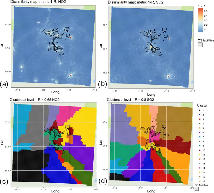
6544                                                                        J. Soares et al.: The use of hierarchical clustering

work (e.g. Lindley, 1956; Rhoades, 1973; Husain and Khan,           (NOx ), photochemical oxidant (Ox ), non-methane hydrocar-
1983; Caselton and Zidek, 1984). Analytical tools such as           bons (NMHC), and PM. In this past work, cluster analysis
Gaussian and Eulerian deterministic dispersion models may           is usually applied to a small number of stations (5 to 70)
also be used to identify possible site locations (e.g. Bauldauf     in different locations around the globe. Solazzo and Gal-
et al., 2002; Mazzeo and Venegas, 2008; Mofarrah and Hu-            marini (2015) applied cluster analysis data showing that clus-
sain, 2009; Zheng et al., 2011). More recently, the spatial         ter analysis can potentially accommodate different sampling
distribution of measured pollutants combined with geostatis-        technologies and could be applied for large areas without the
tical modelling has been used to analyse station data (e.g.         need of prior knowledge of the study area. Note that the data
Cocheo et al., 2008; Lozano et al., 2009; Ferradás et al.,          were pre-filtered by iterative moving averages (Kolmogorov–
2010; Zhuang and Liu, 2011).                                        Zurbenko (KZ) filtering; Zurbenko, 1986) to assess the sim-
   Cluster analysis is a good example of an analysis approach       ilarity of the spectral components of the hourly time se-
which assumes, like many statistical methods, that the data         ries, independent of station location or monitoring technol-
analysed contain a certain degree of redundant information,         ogy employed, without a requirement of prior knowledge
which in turn may be used to describe degrees of similar-           of the study area. Their analysis investigated the extent to
ity or dissimilarity between data records from those stations.      which concentration time series similarities between the air
Typically applied to large and complex air quality databases        quality monitoring stations were defined by areas with spe-
to identify spatial patterns based on a metric describing the       cific chemical regimes and/or predominant air masses versus
degree of (dis)similarity between data time series from dif-        by country borders and/or monitoring network jurisdiction.
ferent stations, cluster analysis (Everitt, et al., 2011) may       The latter were identified as resulting from differences in
be used for source identification and network station density       monitoring methodology, reducing comparability of the data
optimization, with a minimum loss of information (Munn,             across those borders and jurisdictions.
1981). Hierarchical clustering is a well-established associa-          Monitoring of air quality within and downwind of the
tivity analysis methodology used to determine the inherent          oil sands region is a key concern with the provincial and
or natural groupings of objects and/or to provide a summa-          federal governments of Canada. In order to better quantify
rization of data into groups (Johnson and Wicherrn, 2007).          emissions, downwind chemical transformation, and down-
The theoretical basis of hierarchical clustering has the ad-        wind fate of emitted chemicals from this region, the govern-
vantage of making no assumptions regarding the mutual in-           ments of Canada and Alberta set up the Joint Oil Sands Mon-
dependence of samples and does not require examining all            itoring (JOSM) Plan to “improve, consolidate and integrate
clustering possibilities. The similarity among members is es-       the existing disparate monitoring arrangements into a single,
tablished by a distance metric or function, which is used to        transparent government-led approach with a strong scientific
create a similarity matrix in which data are cross-compared         base” (JOSM, 2016). A key part of this overall framework
using the metric. This is followed by operations on the sim-        was to develop methodologies to assess the consistency and
ilarity matrix which group data according to their degree           spatial representativeness of the existing air quality network
of (dis)similarity with respect to that metric. Many studies        of the province of Alberta. The assessment presented here is
have aimed to quantify the spatial similarities among mon-          based on the associativity analysis described in the work of
itoring sites in terms of concentration levels and time vari-       Solazzo and Galmarini (2015) and references therein and fur-
ation by applying, respectively, the Euclidean distance and         ther expands that methodology to focus on monitoring net-
correlation coefficient as similarity metrics. Studies such as      work optimization. We use the methodology for the first time
Lavecchia et al. (1996), Gabusi and Volta (2005), Gramsh et         for observation datasets collected in Alberta, analysing the
al. (2006), Lu et al. (2006), and Giri et al. (2007) applied        data using two different similarity metrics, and rank existing
these metrics for analysing the spatial and temporal distri-        observation stations based on relative station redundancy. We
bution of air contaminants in cities or regions and present         then extend the methodology to a new application of gridded
possible links between those concentrations with specific           air quality model data – showing that time series from a de-
sources, topography, or meteorological patterns. The major-         terministic air quality model (Global Environmental Multi-
ity of these studies focused on ozone (O3 ) and particulate         scale – Modelling Air-quality and Chemistry; GEM-MACH)
matter (PM). Saksena et al. (2003) applied the methodol-            may be used as a surrogate for observations in air quality
ogy to nitrogen dioxide (NO2 ) and sulfur dioxide (SO2 ),           clustering analysis. Dissimilarity may thus be used to rank
Ionescu et al. (2000) to NO2 , Hopke et al. (1976) and McGre-       stations in terms of potential redundancy; here we define re-
gor (1996) to SO2 , and Ignaccolo et al. (2008) to PM10 , NO2 ,     dundancy as the relative dissimilarity level at which a station
and O3 . Cluster analysis has also been suggested for monitor-      joins a cluster. Stations with the lowest levels of dissimilarity
ing network optimization, including station redundancy anal-        may hence be considered sufficiently similar to be considered
ysis in studies such as Ortuño et al. (2005) for CO, Jaimes et      potentially redundant.
al. (2005) and Ibarra-Berastegi et al. (2010) for SO2 , Omar           In addition, we apply the same methodology to time se-
et al. (2005) for aerosol optical properties, Pires et al. (2008)   ries from a deterministic air quality forecast model (GEM-
for O3 and PM, and Iizuka et al. (2014) for nitrogen oxides         MACH) and assess the extent to which the model output can

Atmos. Chem. Phys., 18, 6543–6566, 2018                                              www.atmos-chem-phys.net/18/6543/2018/
J. Soares et al.: The use of hierarchical clustering 6545
be used as a potential surrogate for observations in clustering (WCAS), WBEA, Fort Air Partnership (FAP), Alberta Cap-
analysis. The combined use of the model and clustering anal- ital Airshed Alliance (ACAA), Calgary Regional Airshed
ysis is shown to be a potentially powerful tool for network Zone (CRAZ), Peace Airshed Zone Association (PAZA),
design and/or optimization of existing air quality networks. Palliser Airshed Society (PAS), Parkland Airshed Manage-
We introduce the methodology to assess potential redun- ment Zone (PAMZ), and Lakeland Industrial Community
dancy of monitoring stations (Sect. 2) and describe the ob- Association (LICA). Figure 1b colour codes the sampling
servational and model data used to develop the methodol- site locations by airshed, with continuous station locations
ogy (Sect. 3). In subsequent sections we present the associa- shown as circles and passive stations shown as inverted tri-
tivity analysis for the continuous monitoring (Sect. 4) and angles.
discuss how the methodology can be used to identify differ- Continuous sampling is typically carried out for regula-
ent sampling methodologies (Sect. 5). We then show how tory compliance, where high temporal resolution is required
the same methodology may be used with output from an in order to monitor short-term exceedances in highly variable
air quality model. With favourable comparisons to cluster- concentrations of pollutants in ambient air. The continuous
ing results from air quality monitoring station observations, monitoring principles of ultraviolet pulsed fluorescence and
we show that model output combined with hierarchical clus- chemiluminescence are used to detect and measure SO2 and
tering provides a new approach for monitoring network de- NO2 , respectively, in Alberta, and the maximum value for
sign (Sect. 6). We also discuss potential factors impacting detection limits of the NO2 and SO2 continuous samplers is
the methodology (Sect. 7) and our conclusions are drawn in 1.0 ppbv (AEP, 2014, 2016). In contrast, passive sampling is
Sect. 8. carried out in order to determine monthly average ambient
air concentrations of atmospheric compounds for determina-
tion of long-term trends, to assess of potential ecological ex-
2 Monitoring and air quality model data posure risks, and to understand the spatial distribution of the
measured pollutant. The majority of the Alberta passive mon-
2.1 Study area
itors for NO2 and SO2 were developed by Maxxam Analytics
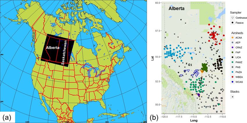
Alberta, one of the western provinces of Canada (Fig. 1), Inc. (Tang et al., 1997, 1999; Tang, 2001), with the excep-
is the largest producer of conventional crude oil, synthetic tion of those employed by PAS (PAS, 2016). The detection
crude and natural gas and gas products in Canada, and is limit for 30-day average NO2 and SO2 sampling periods with
home to one of the world’s largest deposits of oil sand (a these samplers is 0.1 ppbv. We analyse here the data records
mixture of clay, sand, water, and bitumen; CAPP, 2018). The from 39 continuous and 89 passive SO2 monitoring sites and
monitoring of atmospheric pollutants and the provision of 38 continuous and 88 passive NO2 monitoring sites within
public information on air quality in Alberta is carried out the province of Alberta.
by non-profit organizations called “airsheds”; these organiza- Passive sampling techniques have several advantages such
tions are responsible for air pollution monitoring in specified as ease of deployment, no power requirements, and low
subregions of the province. Figure 1b shows the spatial dis- maintenance, and they have been used as an alternative to
tribution of these monitoring networks within the province, continuous monitors for monitoring temporal trends of air
as well as the largest NO2 and SO2 stack emission sources pollutants in remote areas (Krupa and Legge, 2000; Cox,
(National Pollutant Release Inventory, NPRI, 2013). The rel- 2003; Seethapathy et al., 2008; Bytnerowicz et al., 2010)
ative proportion of emissions from different sources depends and evaluation of air quality of large areas (Gerboles et al.,
on the subregion. For example, in the Athabasca oil sands 2006). Their disadvantages are low sensitivity, inability to re-
area (monitored by Wood Buffalo Environmental Associa- solve short-duration concentration peaks, and adverse effects
tion (WBEA) stations; red symbols, Fig. 1b), SO2 is mainly of meteorological conditions on reported observations (Tang
emitted from stacks (flue-gas desulfurization; “major point et al. 1997, 1999; Krupa and Legge, 2000; Tang, 2001; Kirby
sources”) and NO2 is emitted from both stacks and off-road et al., 2001; Partyka et al., 2007; Fraczek et al., 2009; Salem
vehicle mine fleets (“area sources”). The 2013 total emis- et al., 2009; Zabiegala et al., 2010; Vardoulakis et al., 2011).
sions for Alberta were approximately 681 kt for NOx (NO Moreover, the passive monitors depend on monthly meteo-
and NO2 ) and 311 kt for SO2 , respectively. rological information, which are needed in order to calculate
diffusion rates. This information is obtained from the near-
2.2 Monitoring data est site with meteorological observations, as most Alberta
passive sampling sites do not have collocated meteorolog-
In this study we included observations from both passive ical measurements. These constraining factors could influ-
and continuous instruments measuring NO2 and SO2 am- ence the sampling and, therefore, the accuracy of the results,
bient concentrations, since these are the only two species causing under- or overestimation of ambient gas concentra-
in the available data that include observations from both tions in relation to continuous analysers (Krupa and Legge,
measurement methodologies. The nine airsheds within Al- 2000).
berta are shown in Fig. 1b: West Central Airshed Society
www.atmos-chem-phys.net/18/6543/2018/ Atmos. Chem. Phys., 18, 6543–6566, 2018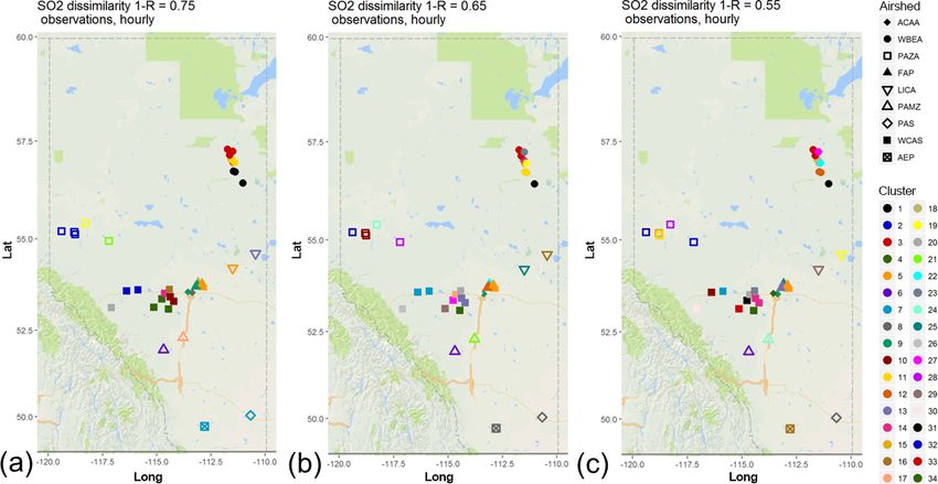
6546                                                                             J. Soares et al.: The use of hierarchical clustering

Figure 1. Study area: (a) model domain covering the provinces of Alberta and Saskatchewan; (b) NO2 and SO2 continuous and passive
monitors located at the different air quality monitoring networks (airsheds) and main NO2 and SO2 stacks in the province of Alberta.
Stations are colour-coded according to airsheds and plotted with different polygons (circle for passive, inverted triangle for continuous):
West Central Airshed Society (WCAS), Wood Buffalo Environmental Association (WBEA), Fort Air Partnership (FAP), Alberta Capital
Airshed Alliance (ACAA), Calgary Regional Airshed Zone (CRAZ), Peace Airshed Zone Association (PAZA), Palliser Airshed Society
(PAS), Parkland Airshed Management Zone (PAMZ), and Lakeland Industrial Community Association (LICA).

   We first analyse the continuous data, reported as hourly             calibration period or stations which came on- or offline dur-
values to Alberta and Environment and Parks (AEP) for the               ing the analysis period. We also follow their recommenda-
period from July 2013 through September 2014, in a manner               tions that data gaps of 1 to 6 h duration are replaced by the
similar to Solazzo and Galmarini (2015), by focusing on the             linear interpolation between the nearest valid data on either
variations associated with different timescales and the deter-          side of the gap and, for data gaps of longer duration, the an-
mination of relative redundancy levels for different continu-           nual average of the non-gap data was used. No substantial
ous monitoring stations. The time period for this continuous-           difference was found between the resulting cluster analysis
only analysis was chosen to overlap with the Environment                by filling the longer gaps with these long-term averages ver-
and Climate Change Canada (ECCC) air quality model sim-                 sus using the average of the same number of missing days
ulations (described further in Sect. 2.3). In a second analysis,        both before and after the gap.
continuous and passive observations encompassing the pe-                   For the comparison between passive and continuous SO2
riod from February 2009 to December 2015 were analysed                  and NO2 observations, the hourly continuous station data
together in an effort to cross-compare the different sampling           records were subject to the same station rejection criteria and
methodologies. The intent of this second analysis was to de-            gap-filling procedures as described above. Passive samplers
termine the extent to which the two methodologies provide               nominally record either 1-month or 2-month averages, de-
similar results, in addition to determining the relative redun-         pending on location. One-month data were averaged to bi-
dancy levels for the passive monitoring stations. In the sec-           monthly data in order to have a consistent time interval for
ond analysis, the continuous data were time-averaged to a               the dataset. When one of the 2-monthly values was missing
similar interval as the passive monitoring data (the passive            from the original data, the bimonthly average was treated
data were typically available as monthly or bimonthly aver-             as missing. Passive stations missing more than 25 % of the
ages).                                                                  data over the 5-year period were rejected from the subse-
   All data were extracted from AEP archives (http://airdata.           quent analysis. This rejection criterion was less stringent than
alberta.ca/, last access: 20 February 2007) and were sub-               that applied to continuous data but was necessary in order to
jected to additional QA–QC procedures due to the require-               achieve a balance between including monitoring sites with
ment of cluster analysis methodologies that there are no gaps           most complete data and attaining good spatial coverage. An
in the time series of observations. We followed the recom-              inclusion criterion of less than 10 % for missing passive data
mendations of Solazzo and Galmarini (2015): continuous                  would have reduced the number of SO2 passive sites in the
station data should be rejected if their hourly data records            analysis from 52 to 18 and NO2 passive sites from 39 to 18.
for the analysis period have more than 10 % of the total data           The missing data were gap-filled using the averages for the
for the year missing or contain data gaps of more than 168              given station for the remainder of the 5-year time period. The
consecutive hours in duration. Missing data may indicate a              gap-filled continuous data for the 5-year period were aver-

Atmos. Chem. Phys., 18, 6543–6566, 2018                                                   www.atmos-chem-phys.net/18/6543/2018/
J. Soares et al.: The use of hierarchical clustering                                                                         6547

aged to the same bimonthly intervals as the passive data. The      then be used as an aid in determining the locations for obser-
monitors included in this study are listed in Tables S1, S2,       vation stations in an optimized monitoring network.
S3, and S4 in the Supplement for the continuous monitoring
network analysis for NO2 and SO2 and passive monitoring
network analysis for NO2 and SO2 , respectively, in Supple-        3     Associativity analysis for monitoring data based on
ment 1.                                                                  dissimilarity

                                                                   3.1    Separating different timescales using KZ filtering
2.3   Modelling output
                                                                   The KZ filter (Zurbenko, 1986) is a means of removing
GEM-MACH (Moran et al., 2010; Makar et al., 2015a, b;              smaller timescales from a time series, based on an iterative
Gong et al., 2015) is an online chemical transport model           moving average over a specific time window. The combina-
describing several air quality processes, including gas-phase      tion of the number of times the moving average is applied (m)
(42 gases), aqueous-phase, and heterogeneous chemistry, and        and the duration of the averaging window (p) determines the
aerosol microphysical processes (nine particle species with        timescales removed from the time series (KZm,p ), following
a two-bin sectional representation in the configuration used       the energy characteristics of the filter. Filtering parameters m
here). GEM-MACH version 2 simulations were carried out             and p can be derived from the transfer function (see Eskridge
for the period between August 2013 and July 2014, over a           et al., 1997, and Zurbenko, 1986, for details on the transfer
domain centred over North America with 10 km grid spac-            function). The removal of high-frequency variations in the
ing. The resulting outputs were used as initial and bound-         data allows different timescales to be isolated and analysed
ary conditions for a nested set of simulations at 2.5 km res-      separately. The KZ filter belongs to the class of low-pass fil-
olution for a domain covering the provinces of Alberta and         ters.
Saskatchewan (Fig. 1a). The model was driven by regulatory            For our analysis, hourly continuous time series data were
reported emissions and additional emissions data emissions         KZ-filtered to remove short timescale variations, resulting in
developed for the model simulations of JOSM (see Zhang et          three additional datasets, which have had filtered-out time
al., 2018, for further details on the model emissions) to better   variations with periods less than a day (KZ17,3 ), a week
simulate Athabasca oil sand surface mining and processing          (KZ95,5 ), and a month (KZ523,3 ). The subsequent analysis
facilities.                                                        may thus examine the effect of removing the signal of the
   GEM-MACH simulations have been previously evaluated             different timescales on the relationships between the stations.
for both NO2 and SO2 concentrations against monitoring net-        The time series resulting from each level of filtering may then
work data and satellite observations and cross-compared to         be cross-compared, using hierarchical clustering, described
the output of other air quality models in Im et al. (2015),        in the following section.
Wang et al. (2015), Makar et al. (2015a, b), and Moran                In previous work appearing in the literature (Solazzo and
et al. (2016). Further evaluation of GEM-MACH on the               Galmarini, 2015), the KZ filter was used in a “band-pass”
high-resolution domain used here can be found in Makar et          configuration. A “band pass” is the difference between two
al. (2018) and Akingunola et al. (2018).                           KZ filters, for two different frequencies, and was used in an
   We use the output from GEM-MACH in two ways: ini-               attempt to isolate the energy between those two frequencies.
tially, hourly 2.5 km resolution model results were extracted      However, Hogrefe et al. (2000, 2003) indicated that applying
at monitoring station locations, and then cluster analyses for     the difference in KZ filters for band-pass purposes does not
the model and observation data were compared. This com-            separate the spectral components completely, with the energy
parison was carried out in order to evaluate the extent to         spectrum overlapping between the neighbour components.
which the model could act as a proxy for the observations          Rather than each band defining an exclusive set of frequen-
and provide any caveats on the observation analysis associ-        cies, some of the energy from one band could be detected
ated with time averaging, sampling errors, and accuracy of         by the neighbouring band. We carried out a detailed analy-
the observations. In our final analysis, we demonstrate the        sis of the band-pass configuration and confirmed the analysis
use of the model as a proxy for monitoring network design          of Hogrefe et al., further finding that this energy “leakage”
by treating every model grid cell as if it contained a moni-       between bands was sufficient that the frequency bands asso-
toring station – the clustering analysis of this proxy “data”      ciated with the shorter timescales could not be distinguished
was then used to define subregions within the model domain         from each other. However, the KZ filter in its original low-
which could be represented by a single station for different       pass form was found to be able to separate the timescales in
values of the clustering metric. We carried out this analysis      the test data accurately, simply by choosing m and p coeffi-
on a 36-by-36 test cell subdomain centred on the Athabasca         cients to ensure that all energy was removed below specific
oil sands, but the methodology could be scaled to larger re-       frequencies. Subsequent clustering was shown to distinguish
gions. The results of this final analysis are spatial maps at      the influence of the different timescales, given an appropri-
different levels of a given dissimilarity metric, which may        ate choice of the filtering parameters m and p. Our detailed

www.atmos-chem-phys.net/18/6543/2018/                                               Atmos. Chem. Phys., 18, 6543–6566, 2018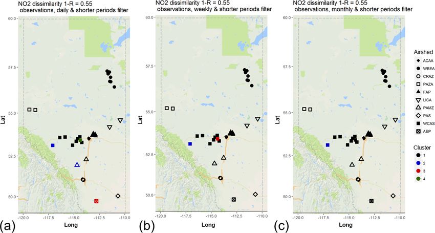
6548 J. Soares et al.: The use of hierarchical clustering
analysis of the KZ filter in low-pass and band-pass configu- could be considered redundant despite the information in-
rations is described in detail in Supplement 2. Note that the herent in the lower concentrations associated with increas-
m and p values used in this study were chosen to give an ing distance from the emissions source. For both metrics, the
equivalent impact as band-pass filters used in Solazzo and recalculation of the dissimilarity matrix is carried out here
Galmarini (2015). with the general averaging method (Næs et al., 2010), as it
It should be noted that time filtering and time averaging provides robust and accurate clustering, with a substantial re-
do not provide the same information. In the case of low-pass duction in the processing time required to generate clusters
time filtering, the higher-frequency variation above some fre- (Solazzo and Galmarini, 2015).
quency is removed from the time series, while in the case of The level of dissimilarity at which individual station
averaging that information is added to the average. records, and then clusters of records, merge as each new clus-
ter is called a “node”. The order in which station records
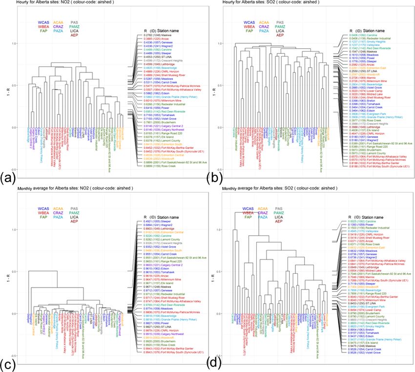
3.2 Dissimilarity analysis using hierarchical clustering merge, as well as the level of dissimilarity at which they
merge, may be displayed in diagrams known as dendro-
“Dissimilarity analysis” encompasses a group of methodolo- grams. Dendrograms show the pattern of linkages between
gies used to rank datasets based on the extent to which they nodes as the analysis progressed, with the vertical axis rep-
are different (or dissimilar) from each other. Dissimilarity resenting the level of dissimilarity, vertical lines represent-
may thus be used to rank stations in terms of potential redun- ing specific clusters, and horizontal lines joining the clusters
dancy such that stations with low levels of dissimilarity may representing the nodes where the clusters are linked. A den-
be similar enough to be redundant. One of the most com- drogram has the appearance of the roots of a tree, with the
monly used methodologies for dissimilarity analysis is hier- join between the lowest roots representing the node of the
archical clustering (Johnson and Wicherrn, 2007). most similar time series and the trunk of the tree the point
The first step for hierarchical clustering is to choose a met- at which all data have been joined to clusters. Very similar
ric to describe how dissimilar the time series are from each stations are thus joined at the bottom of a dendrogram.
other. This metric is then calculated for all possible pairs of
the time series comprising the dataset. This initial set of cal- 3.3 Assessing potential station redundancy
culations results in a dissimilarity matrix, which may then be
used to cluster the data, based on the level of dissimilarity. Hierarchical clustering as described above was used to as-
The pair of time series with the lowest level of dissimilarity sist in the evaluation of potential monitoring station redun-
is combined and forms the first cluster. The metric of dis- dancies (defined as the relative dissimilarity level at which
similarity is then recalculated between the first cluster and a station joins a cluster), as one of many considerations that
the remaining time series, followed by pairing time series could influence decision-making on monitoring network de-
and/or clusters with the lowest dissimilarity in the reduced sign. Having carried out hierarchical clustering using station
matrix. The number of clusters, which was originally equal data, the values of the dissimilarity metric as stations join
to the number of time series in the original dataset, is thus clusters may be used to define the extent of similarity be-
reduced at each stage of the hierarchical clustering process; tween stations, as well as a relative ranking of stations based
the process will be completed when the two last clusters have on these similarities. This provides a quick assessment of sta-
joined. tion record similarities and offers insight into how the records
In this work, we have used two dissimilarity metrics: are related to each other with respect to their temporal vari-
(1) 1 − R, where R is the Pearson linear correlation coef- ations (1 − R) and magnitudes (Euclidean distance) through-
ficient (Solazzo and Gamarini, 2015), and (2) the Euclidean out the time interval analysed. We would consider stations
distance (the latter is the square root of the sum of the squares potentially redundant if stations highly correlate with each
of the differences between the two time series’ members). other (low 1 − R levels) and if the Euclidean distance levels
The metric based on correlation assesses dissimilarities as- are low. To decide if stations are redundant or not, a level of
sociated with the changes in concentration as a function of 1−R and/or Euclidean distance should be set; all the stations
time, while the Euclidian distance metric assesses dissimi- clustering under the same cluster at that given level should be
larities on the basis of magnitude, over the time period of the under consideration for being removed or moved.
analysis. We included the Euclidean distance out of concern An assessment of monitoring record redundancies must
that 1 − R alone would fail to assess the magnitude differ- be made prudently, the metrics used should be carefully as-
ences, which may be more important than correlation, for sessed, and the physical distance between the stations and
some monitoring network applications. An extreme example emissions sources should be taken into consideration (see
would be two perfectly correlated time series, one of which Sect. 7). The inherent limitations of the analysis should also
has average concentrations an order of magnitude lower than be noted. These include the following:
the first; such a comparison could result from two stations 1. The ranking of stations is relative and specific to a given
positioned at different distances in a line downwind from an chemical species, the corresponding set of station time
emissions source. Using 1 − R alone, one of these stations series, and the parameters used for the hierarchical clus-
Atmos. Chem. Phys., 18, 6543–6566, 2018 www.atmos-chem-phys.net/18/6543/2018/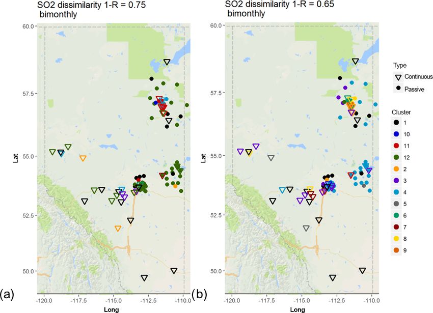
J. Soares et al.: The use of hierarchical clustering                                                                        6549

     ter analysis: metric of dissimilarity and the method to      4     Dissimilarity analysis for the continuous monitoring
     recalculate the dissimilarity matrix.                              networks in Alberta
 2. Stations excluded because of data incompleteness are
                                                                  4.1    Spatial distribution of clusters
    not analysed and not evaluated for possible redundan-
    cies.
                                                                  The dissimilarity analysis was applied to NO2 and SO2 ob-
 3. The methodology has been applied in the past using            servational time series data for all the stations complying
    observations from existing monitoring stations in or-         with the QA–QC criteria described in Sect. 2. The dendro-
    der to analyse the relative dissimilarity between those       grams resulting from the analysis are provided in Supple-
    stations’ data records. However, the methodology may          ment 1.
    also be applied to gridded model-generated concentra-            The hierarchical clustering results for NO2 using 1 − R
    tion time series. The latter application provides informa-    as the dissimilarity metric are depicted in Fig. S1 in the
    tion on possible new locations for monitoring stations        Supplement. This NO2 dendrogram shows frequent cluster-
    for a given number of monitoring stations or dissimi-         ing between stations within the same airshed (if represented
    larity level (this process is described in more detail in     by more than a single station) or airsheds that are in rela-
    Sect. 6).                                                     tively close physical proximity, such as airsheds ACAA and
                                                                  FAP (see Fig. 1b). A horizontal line cutting across a den-
 4. Other considerations may factor strongly into moni-           drogram such as Fig. S1 may be used to define the station
    toring network decision redundancy: for example, the          records that are part of a cluster at a given level of the dis-
    availability of roads and electrical power, regulatory re-    similarity metric, and these may be plotted spatially: Fig. 2
    quirements, and cost.                                         shows the spatial distribution of the clusters of NO2 continu-
An important corollary to the first point above is that dif-      ous monitors at three levels of the 1 − R dissimilarity metric:
ferent methods used in hierarchical clustering may result in      0.75 (Fig. 2a), 0.65 (Fig. 2b), and 0.55 (Fig. 2c). The results
different relative rankings of station records. Station records   show that stations tend to cluster over successively smaller
which are highly similar when 1 − R is used (this metric is       areas as the level of dissimilarity decreases (the three clus-
unitless and zero (unity) for the most (least) similar time se-   ters of Fig. 2a as dissimilarity decreases become 11 clusters
ries or clusters) may be highly dissimilar when the Euclidean     by Fig. 2c). The clustering at high dissimilarity levels (aka
distance is used (the Euclidean distance will have units of       low correlation coefficients) also allows anomalous group-
the chemical species being analysed and will be zero for the      ings of stations. For example, cluster 1 in Fig. 2a includes
most similar clusters, but the magnitude of the upper limit       both WBEA stations at the upper right of the panel, one
of dissimilarity will depend on the specific time series being    WCAS and one PAMZ station, despite the latter two sam-
clustered).                                                       pling air in other parts of the province and being subject to
   “Redundancy” with regards to the metrics examined here         different sources. This tendency is reduced at lower levels
is thus relative to a given chemical species and dataset used     of dissimilarity, where stations influenced by similar sources
for hierarchical clustering. Therefore, we do not propose spe-    tend to cluster. For example, in Fig. 2c, cluster 8 includes
cific thresholds of the two metrics for determining redun-        all the stations in a highly urbanized area (Edmonton, capital
dancy. We note also that the results of the analyses for two      city of the province) and cluster 11 is a station located at a
metrics may be combined – station data that are relatively        relatively high elevation upwind of most emission sources.
similar under one metric may be examined for their degree         Overall, the methodology shows the ability to group together
of similarity under another metric. The metric levels at which    monitoring station locations which might be expected to be
these combinations are examined are themselves also quali-        influenced by similar sources of emissions.
tative, but station time series which are highly similar under       We next examine how the timescales inherent in the
multiple metrics are in turn a stronger indication of potential   data may affect similarities. Figure 3 shows the clustering
redundancy.                                                       of stations which occurs at a 1 − R dissimilarity level of
   Despite the above limitations, the methodology is never-       0.55 after timescales less than daily (Fig. 3a, dendrogram
theless highly useful. In the event of limited available re-      in Fig. S2), weekly (Fig. 3b, dendrogram in Fig. S3), and
sources for monitoring, an assessment of relative redun-          monthly (Fig. 3c, dendrogram in Fig. S4) are removed. Four
dancy, through the use of more than one metric, may aid in        clusters are shown on the first panel, three on the second, and
decision-making. Aside from implying redundancy between           two on the third. Comparing back to Fig. 2c with the original
two data records, a high level of similarity may also indicate    hourly data, this shows that much of the “signal” in 1 − R
that a station may provide more information to the network        contributing to the 11 clusters in Fig. 2c is contained within
if placed elsewhere, as opposed to its current location. In the   the shorter timescales of less than a day and are relatively
last part of the analysis (Sect. 6), we show how the method-      similar at longer timescales. Moreover, correlation levels be-
ology may be extended through the use of air quality model        tween stations increase as KZ filtering is applied and shorter
output to design dissimilarity-optimized air quality networks.    time variability is removed. All of this evidence indicates that

www.atmos-chem-phys.net/18/6543/2018/                                              Atmos. Chem. Phys., 18, 6543–6566, 2018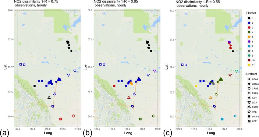
6550                                                                                 J. Soares et al.: The use of hierarchical clustering

Figure 2. Associativity analysis for observed NO2 hourly time series using 1−R as the metric to compute the dissimilarity matrix, assuming
a dissimilarity level of (a) 0.75, (b) 0.65, and (c) 0.55. Stations are colour-coded by cluster, and airsheds are plotted with different polygons.
The acronyms for the airsheds are as in Fig. 1.

Figure 3. Associativity analysis for observed NO2 filtered time series using 1−R as the metric to compute the dissimilarity matrix, assuming
a dissimilarity level of 0.55: (a) daily, (b) weekly, and (c) monthly and short time periods. Stations are colour-coded according to cluster
formation, and airsheds are plotted with different polygons. The acronyms for the airsheds are as in Fig. 1.

much of the variation in NO2 in the region takes place on rel-             stations even when timescales of less than a month are re-
atively short timescales and is due to local sources. The anal-            moved from the analysis.
ysis also indicates that some stations are more influenced by                 The dissimilarity analysis for SO2 produced different re-
seasonality than others; e.g. the high altitude, largely upwind            sults from that for NO2 . Figure 4 shows the spatial distribu-
site of cluster 2 in Fig. 3c, remains separate from the other              tion of the clusters of SO2 continuous monitors with the 1−R
                                                                           dissimilarity metric (the dendrogram resulting from the hier-

Atmos. Chem. Phys., 18, 6543–6566, 2018                                                        www.atmos-chem-phys.net/18/6543/2018/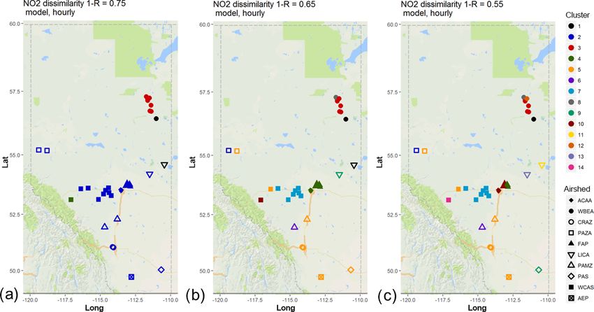
J. Soares et al.: The use of hierarchical clustering 6551
Figure 4. Associativity analysis for observed SO2 hourly time series using 1 − R as the metric to compute the dissimilarity matrix, assuming
a dissimilarity level of (a) 0.75, (b) 0.65, and (c) 0.55. Stations are colour-coded by cluster, and airsheds are plotted with different polygons.
The acronyms for the airsheds are as in Fig. 1.
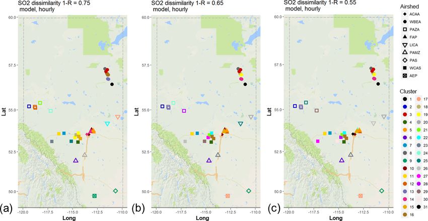
archical clustering appears in Fig. S5) and can be compared The Euclidean distance dendrograms for both NO2
to Fig. 2. For a given level of 1 −R, there are more SO2 clus- (Fig. S9) and SO2 (Fig. S10) do not show the same distinc-
ters than NO2 clusters. The observations of SO2 , despite be- tive clustering within airsheds as can be seen with the 1 − R
ing largely collocated with the observations of NO2 , are nev- metric. This might be expected, as Euclidean distance be-
ertheless more dissimilar than the observations of NO2 . Even tween two time series may result from a single instance in
at higher levels of dissimilarity (compare Figs. 2a and 4a), which the hourly concentration records of the two stations
there are more SO2 clusters, indicating a greater degree of differ substantially or several hours in which the concen-
local variability in the SO2 data, which drives correlation co- tration differences are smaller. Stations located sufficiently
efficients lower and dissimilarity levels for the 1 − R metric far apart that they monitor different sources of pollutants
higher. This greater degree of dissimilarity for SO2 is due to may thus have similar Euclidean distances if their average
the nature of the SO2 emissions, i.e. almost exclusively from concentration magnitude is similar. The analysis also indi-
industrial “point” sources in the region under study, whereas cates that Euclidean distances become more similar in mag-
NO2 concentrations are also influenced by more broadly ge- nitude and that these magnitudes decrease, as increasingly
ographically dispersed “area” sources of emissions includ- larger timescales are filtered, across all of Alberta (Fig. S9
ing mobile on- and off-road vehicles. The dispersion of SO2 for NO2 and Fig. S10 for SO2 ). That is, concentration mag-
from the former source type is thus more dependent on very nitudes recorded at the different stations approach each other
local meteorological conditions governing the rise of buoyant as the shorter-duration time variations are removed. At these
plumes from stacks than are the emissions from area sources. timescales, the magnitude of both species is driven by low
The direction and concentration of the rising and dispersing concentration levels of long-term duration and larger spatial
SO2 plumes are thus more highly variable in time compared extent. This is particularly true for SO2 monitors that typi-
to the area-source-dominated emissions of NO, which are cally measure low concentration (background levels) inter-
chemically transformed rapidly to NO2 . Concentrations from spersed with infrequent short-term high concentrations (sur-
the same SO2 source may therefore not correlate to the same face fumigation events of buoyant plumes). However, within
degree between different downwind stations as NO2 . This an airsheds affected by a common set of emissions sources,
contributes to the lesser degree of similarity between the SO2 Euclidean distance will nevertheless be useful by identify-
station data even when monthly and shorter timescales are re- ing the presence of high-concentration gradients, as will be
moved (the SO2 dendrograms with the removal of timescales shown in the next section.
less than daily, weekly, and monthly appear in Figs. S6, S7, In summary, the methodology is able to identify groups of
and S8, respectively). stations which are influenced by common emissions sources
(e.g. stations which are influenced by oil sand emissions as
www.atmos-chem-phys.net/18/6543/2018/ Atmos. Chem. Phys., 18, 6543–6566, 2018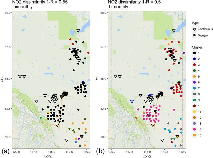
6552                                                                           J. Soares et al.: The use of hierarchical clustering

Table 1. Hourly NO2 similarity ranking for the 1 − R and Euclidean distance (EuD) metrics. Note that stations at the bottom of the two
columns are the most similar (hence one measure of their level of redundancy) with respect to each metric of dissimilarity. Here we show
only the first 10 and last 10 items of the ranking; the full ranking can be consulted in Table S5.

         1−R      Name                            ID   Airshed     EuD    Name                                   ID   Airshed
         0.72     Maskwa                       1248    LICA       1009    Shell Muskeg River                  1244    WBEA
         0.61     Anzac                        1225    WBEA        950    Millennium Mine                     1075    WBEA
         0.60     ST.LINA                      1250    LICA        950    Fort McMurray Athabasca Valley      1064    WBEA
         0.56     Steeper                      1055    WCAS        923    Grande Prairie (Henry Pirker)       1165    PAZA
         0.56     Caroline                     1092    PAMZ        839    Calgary Northwest                   1039    CRAZ
         0.55     Lethbridge                   1049    AEP         839    Calgary Central 2                   1221    CRAZ
         0.55     Crescent Heights             1172    PAS         807    Redwater Industrial                 1156    FAP
         0.54     Wagner2                      1241    WCAS        769    Red Deer Riverside                  1142    PAMZ
         0.54     Genesee                      1057    WCAS        735    Edson                               1062    WCAS
         0.51     Shell Muskeg River           1244    WBEA        722    Meadows                             1058    WCAS
         0.18     Range Road 220               1161    FAP         400    Fort Saskatchewan                   2001    FAP
         0.16     Lamont County                1162    FAP         387    Anzac                               1225    WBEA
         0.16     Elk Island                   1157    FAP         350    Violet Grove                        1052    WCAS
         0.16     Fort McKay South             1076    WBEA        350    Tomahawk                            1053    WCAS
         0.16     Fort McKay Bertha Ganter     1032    WBEA        348    Power                               1059    WCAS
         0.15     Edmonton Central             1028    ACCA        301    Caroline                            1092    PAMZ
         0.14     Woodcroft                    2002    ACCA        280    Steeper                             1055    WCAS
         0.14     Edmonton South               1036    ACCA        280    ST.LINA                             1250    LICA
         0.11     Ross Creek                   1159    FAP         263    Lamont County                       1162    FAP
         0.11     Fort Saskatchewan            2001    FAP         263    Elk Island                          1157    FAP

opposed to stations located elsewhere) when the methodol-             timescales of less than 5 min) produced from their primary
ogy is applied to hourly and, to some extent, daily time-             precursors, much of the signal driving similarity resides at
filtered time series. Stations mainly influenced by seasonal-         shorter timescales. Consequently, our ranking of continuous
ity are identified when the methodology is applied to weekly          monitoring stations in this section is based solely on the orig-
and monthly time-filtered data. The analysis groups stations          inal hourly observation data, as opposed to KZ-filtered obser-
according to their degree of similarity but does not provide          vations.
the cause for that degree of similarity. The latter may only be          The cluster analysis results for hourly time series were
achieved by examination of the data records and the use of            ranked from highest to lowest values of 1 − R and Euclidean
local knowledge of sources and conditions. The level of in-           distance resulting from clustering of continuous monitoring
formation about the sources present in the study area will be         station data. Stations clustering at high levels of 1 − R and
greater when the results of both metrics are combined, and            Euclidean distances are significantly different in time varia-
information about the sources may be inferred from the anal-          tion and concentration magnitudes, respectively. Conversely,
ysis; for example, stations could be classified as background         stations at the bottom of the ranking are the most similar.
or industrial impacted if seasonality or hourly data are shown        The latter stations could be, therefore, considered potentially
to contain most of the signal.                                        redundant. Our rankings are based on the dissimilarity level
                                                                      at which a given station joins another station as a new clus-
4.2    Ranking of stations by dissimilarity                           ter or when a given station joins a pre-existing cluster. If the
                                                                      latter were to occur at a sufficiently low level of dissimilar-
Previous work appearing in the literature (Solazzo and                ity, either the new station or the pre-existing cluster might be
Gamarini, 2015) was motivated by the aims of evaluation               considered potentially redundant. The uppermost and lower-
and pre-screening of monitoring data for the purpose of the           most ranked stations for NO2 and SO2 are shown in Tables 1
evaluation and development of regional-scale air pollution            and 2, respectively. The corresponding full ranking for the
models. Their focus was on observations of ozone, which,              full list of stations is shown in Tables S5 and S6.
in the troposphere, is a secondary pollutant resulting from              The tabulated values indicate clear differences between the
gas-phase reactions and broader-scale chemistry and trans-            two compounds. The stations measuring NO2 cluster with
port. They consequently focused on the different timescales           each other at substantially lower 1−R levels (that is, they cor-
associated with KZ filtering. Here, however, we have shown            relate at substantially higher values of R) than do the stations
that for primary pollutants such as SO2 and “secondary” pol-          measuring SO2 . In one extreme case, the records of one SO2
lutants such as NO2 , which are nevertheless very rapidly (on         station, Redwater Industrial, anti-correlate with the records

Atmos. Chem. Phys., 18, 6543–6566, 2018                                                 www.atmos-chem-phys.net/18/6543/2018/
J. Soares et al.: The use of hierarchical clustering 6553 of other stations, indicating that the SO2 time series at that 5 Hierarchical clustering to cross-compare location is substantially different from those of the remaining methodologies and technologies stations. However, the NO2 Euclidean distance metric cluster values tend to form at higher levels than their SO2 counter- parts, with the exception of Redwater Industrial, indicating Solazzo and Galmarini (2015) noted that clustering analy- that despite their higher correlations, the NO2 stations may sis can be used to determine the extent to which the differ- have larger differences in concentration magnitudes relative ent monitoring methodologies are comparable. Thus if differ- to SO2 . We note that the Euclidean distance between SO2 ent methodologies do not provide equivalent data, the clus- station observations is, in many cases, relatively low (e.g. ters generated will be split according to methodology rather 24 ppbv for 8760 hourly values summed) and likely indi- than being associated with local chemical and meteorolog- cates stations which rarely record SO2 concentrations above ical conditions. The combination of monitoring methodolo- background levels and hence have relatively “similar” Eu- gies here thus has two purposes – to assess the relative dis- clidean distances due to similarly low-concentration records similarities between station records and to verify that both for much of the recorded time series. Another interesting dif- passive and continuous monitors provide similar data. ference between the two atmospheric compounds is that the The hierarchical clustering methodology was applied to relative ranking by dissimilarity is closer to being the same the 5-year bimonthly averaged time series sampled by con- for the two metrics for SO2 than for NO2 . tinuous and passive monitors (we leave out the a priori KZ Two different dissimilarity metrics thus result in different filtering step as the data in this case are already long-term av- relative rankings of the two chemical species, so the results erages). The dendrograms resulting from the clustering anal- must be interpreted with care. For example, the stations Fort ysis are shown in Fig. S11 for NO2 and Fig. S12 for SO2 . McKay South and Fort McKay Bertha Ganter have the high- The spatial distributions for the station clusters for the 1 − R est correlation for SO2 (R = 0.81) but their Euclidean dis- dissimilarity metric will be the focus here. tance is 177 ppbv, and a similar disparity between 1 − R and The spatial distributions of the NO2 clusters at dissimi- Euclidean distance rankings for these stations may be seen larity levels of 1 − R = 0.55 and 0.5 are shown in Fig. 5a in their values of the corresponding NO2 metrics (R = 0.84 and b, respectively, with the locations of continuous moni- and Euclidean distance of 411 ppbv). These stations are 4 km tors plotted as inverted triangles and passive monitors as cir- apart; the high correlation coefficients indicate that they may cles. At correlation level R = 0.45 (Fig. 5a) there is a clear measure similar events, but the high Euclidean distances in- distinction between passive and continuous monitors; all the dicate that the magnitude of the events observed likely varies continuous monitors belong to cluster 1, independent of their considerably despite the small separation distance. That is, spatial location. A large number of the passive monitors also substantial gradients in concentration may exist between the fall within this cluster; however, when a slight increase in two stations at any given time. We note again here that low correlation is applied (Fig. 5, R = 0.5), the clustering pattern values of the dissimilarity metrics indicate a greater level of changes significantly – most of the continuous monitors re- potential redundancy with respect to the rest of the stations main within the same cluster, but the passive monitors form – a high value of the Euclidean distance between two sta- separate clusters. Two WCAS continuous monitors separate tion records, or between a station record and a cluster, in- and form a separate cluster at dissimilarity level 0.5 (Fig. 5b). dicates that they are very dissimilar, and hence less poten- Figure 5 also shows several cases of collocated continuous tially redundant. A second example is the pair of stations and passive monitors which do not fall within the same clus- measuring NO2 with the lowest 1 − R, Ross Creek and Fort ter for correlation levels of 0.5 or higher. The analysis shows Saskatchewan: these stations’ data records are highly simi- that as higher levels of correlation are required, the contin- lar with respect to 1 − R (that is, they are highly correlated), uous and passive monitors for NO2 do not cluster together but the Euclidean distance between the two is 400 ppbv de- despite close physical proximity or even collocation. Some spite the stations being separated in distance by only 2.6 km. of the passive monitor clusters at R = 0.5 (Fig. 5b) appear Again, the gradients in concentration between closely placed anomalous; for example, cluster 3 (red) includes stations in stations can be substantial. The intended purpose of the mon- LICA and WBEA, despite these airsheds being separated by itoring at such locations is key to assessing their level of a distance of several hundred kilometres. As the level of dis- potential redundancy. For example, if the aim of monitoring similarity is decreased from 0.55 to 0.5, the biggest differ- is to provide short-term exposure data for human health im- ence in clustering patters is seen for WBEA monitors (in the pacts, then these large Euclidean distances (despite the high upper right of the panels of Fig. 5) as passive and continuous correlations) indicate the presence of large gradients in con- monitors located closer to the oil sands facilities fall within centration, and hence such station pairs should be considered cluster 1, while some of the passive monitors farther from the less redundant. The combination of the metrics is thus shown oil sands facilities fall within cluster 3. For levels of correla- to be important in network assessment – the addition of the tion above 0.5, the clustering between stations monitoring Eulerian distance metric provides a broader context for sta- similar source areas is rare, independent of the airsheds (see tion ranking than the use of 1 − R alone. dendrogram in Fig. S8). www.atmos-chem-phys.net/18/6543/2018/ Atmos. Chem. Phys., 18, 6543–6566, 2018
6554                                                                                J. Soares et al.: The use of hierarchical clustering

Table 2. Hourly SO2 similarity ranking. Note that stations at the bottom of the two columns are the most similar (hence one measure of their
level of redundancy) with respect to each metric of dissimilarity. Here are only the first and last 10 items of the ranking; the full ranking can
be consulted in Table S6.

        1−R      Name                                     ID    Airshed      EuD     Name                                 ID    Airshed
        1.01     Redwater Industrial                    1156    FAP         1594     Redwater Industrial               1156     FAP
        0.95     Caroline                               1092    PAMZ         709     Mannix                            1069     WBEA
        0.88     Valleyview                             1170    PAZA         532     Mildred Lake                      1066     WBEA
        0.88     Smoky Heights                          1167    PAZA         470     Millennium Mine                   1075     WBEA
        0.85     Maskwa                                 1248    LICA         412     Shell Muskeg River                1244     WBEA
        0.85     Mannix                                 1069    WBEA         372     Lower Camp                        1074     WBEA
        0.83     Red Deer Riverside                     1142    PAMZ         269     CNRL Horizon                      1226     WBEA
        0.81     Steeper                                1055    WCAS         231     Wagner2                           1241     WCAS
        0.81     Power                                  1059    WCAS         231     Genesee                           1057     WCAS
        0.81     Meadows                                1058    WCAS         220     Edmonton East                     1029     ACCA
        1.01     Redwater Industrial                    1156    FAP          215     Maskwa                            1248     LICA
        0.48     Wagner2                                1241    WCAS         102     Caroline                          1092     PAMZ
        0.48     Genesee                                1057    WCAS          91     Smoky Heights                     1167     PAZA
        0.45     Range Road 220                         1161    FAP           79     Carrot Creek                      1054     WCAS
        0.45     Fort Saskatchewan                      2001    FAP           70     Lethbridge                        1049     CRAZ
        0.39     Lamont County                          1162    FAP           58     Beaverlodge                       1168     PAZA
        0.39     Bruderheim                             2000    FAP           55     Grande Prairie (Henry Pirker)     1165     PAZA
        0.35     Fort McMurray Patricia McInnes         1070    WBEA          50     Crescent Heights                  1172     PAS
        0.35     Fort McMurray Athabasca Valley         1064    WBEA          42     Evergreen Park                    1166     PAZA
        0.19     Fort McKay South                       1076    WBEA          24     Steeper                           1055     WCAS
        0.19     Fort McKay Bertha Ganter               1032    WBEA          24     Red Deer Riverside                1142     PAMZ

   Figure 6 depicts the clustering results for SO2 based on                collocated passive and continuous monitors for SO2 do not
the 1 − R metric for dissimilarity levels 0.75 (Fig. 8a) and               fall within the same cluster at lower 1 − R values (these are
0.65 (Fig. 8b). Higher dissimilarity levels were used as ex-               shown as different colours in overlapping inverted triangles
amples for the generation of spatial distributions than for                and circles in Fig. 6b). This indicates that at least some of
NO2 in this figure. The highly variable nature of the SO2                  the variability may reside in the measurement methodologies
concentrations, as a result of their origin in stack emissions,            employed.
results in a greater degree of variability inherent in the col-               In their analysis of European ozone monitoring networks,
lected data, as described earlier (at lower dissimilarity lev-             Solazzo and Galmarini (2015) found similar patterns be-
els, the number of clusters increases markedly). Comparing                 tween different European nations, noting that the differences
Figs. S9 and 6, most of WBEA passive and continuous mon-                   are likely related to different sampling methodologies, instru-
itors in the north-east of the region form a common cluster at             ment sensitivities, and data acquisition protocols not being
R = 0.25 (Fig. 6a, cluster 11, red). However, at this low cor-             harmonized between the countries. The same seems to be
relation level, a common cluster connects sites in LICA, FAP,              true for the Alberta passive and continuous monitoring sta-
WBEA, and PAZA airsheds, despite these sites being widely                  tions, as the 1 − R cluster analysis shows that the continuous
separated in space and influenced by different local sources               stations are more similar to each other within and across air-
of SO2 (cluster 12, green, Fig. 6a). At the slightly higher cor-           sheds than they are to the passive stations within the same
relation level of R = 0.35 (Fig. 6b), the clustering across air-           airsheds, or located nearby. Collocated continuous and pas-
sheds has been reduced, though LICA and FAP still share a                  sive stations do not always show high levels of similarity,
common cluster (number 4, light blue). Again, the most di-                 which would be expected had they reported the same con-
rect interpretation of the differences between the SO2 and                 centrations. We analysed WBEA data alone using the 1 − R
NO2 results for the 1 − R metric analysis, when passive and                metric (dendrogram in Fig. S13) and found that most of the
continuous monitors are clustered together, is that the data               continuous monitors formed a separate cluster from the pas-
time series records for SO2 are more highly variable than for              sive monitors at relatively high levels of the 1 − R metric, in-
NO2 . If 1−R similarity is used for assessing potential station            dicating that the two sources of data provide fundamentally
redundancies, then there is a lesser overall degree of poten-              different records. Collocated passive and continuous moni-
tial redundancy in the SO2 data due to its greater degree of               tors also tended to have high levels of the Euclidean distance
variability. However, the cause of that variability should also            (not shown). Thus, at least some of the variability noted with
be considered. For example, we note again that some of the                 these datasets seems to lie with the overall sampling method-

Atmos. Chem. Phys., 18, 6543–6566, 2018                                                       www.atmos-chem-phys.net/18/6543/2018/
You can also read


