WAP-1D-VAR v1.0: development and evaluation of a one-dimensional variational data assimilation model for the marine ecosystem along the West ...
←
→
Page content transcription
If your browser does not render page correctly, please read the page content below
Geosci. Model Dev., 14, 4939–4975, 2021
https://doi.org/10.5194/gmd-14-4939-2021
© Author(s) 2021. This work is distributed under
the Creative Commons Attribution 4.0 License.

WAP-1D-VAR v1.0: development and evaluation of a
one-dimensional variational data assimilation model for the marine
ecosystem along the West Antarctic Peninsula
Hyewon Heather Kim1,2 , Ya-Wei Luo3 , Hugh W. Ducklow4 , Oscar M. Schofield5 , Deborah K. Steinberg6 , and
Scott C. Doney2
1 Woods  Hole Oceanographic Institution, Woods Hole, MA 02543, USA
2 University of Virginia, Charlottesville, VA 22904, USA
3 Xiamen University, Xiamen, Fujian 361102, China
4 Lamont-Doherty Earth Observatory, Columbia University, Palisades, NY 10964, USA
5 Rutgers University, New Brunswick, NJ 80901, USA
6 Virginia Institute of Marine Science, Gloucester Point, VA 23062, USA

Correspondence: Hyewon Heather Kim (hkim@whoi.edu)

Received: 11 November 2020 – Discussion started: 4 February 2021
Revised: 14 June 2021 – Accepted: 21 June 2021 – Published: 12 August 2021

Abstract. The West Antarctic Peninsula (WAP) is a rapidly      optimization, via an optimized set of 12 parameters out of
warming region, with substantial ecological and biogeo-        a total of 72 free parameters. The optimized model results
chemical responses to the observed change and variability      capture key WAP ecological features, such as blooms during
for the past decades, revealed by multi-decadal observations   seasonal sea-ice retreat, the lack of macronutrient limitation,
from the Palmer Antarctica Long-Term Ecological Research       and modeled variables and flows comparable to other studies
(LTER) program. The wealth of these long-term observations     in the WAP region, as well as several important ecosystem
provides an important resource for ecosystem modeling, but     metrics. One exception is that the model slightly underesti-
there has been a lack of focus on the development of nu-       mates particle export flux, for which we discuss potential un-
merical models that simulate time-evolving plankton dynam-     derlying reasons. The data assimilation scheme of the WAP-
ics over the austral growth season along the coastal WAP.      1D-VAR model enables the available observational data to
Here, we introduce a one-dimensional variational data assim-   constrain previously poorly understood processes, including
ilation planktonic ecosystem model (i.e., the WAP-1D-VAR       the partitioning of primary production by different phyto-
v1.0 model) equipped with a model parameter optimization       plankton groups, the optimal chlorophyll-to-carbon ratio of
scheme. We first demonstrate the modified and newly added      the WAP phytoplankton community, and the partitioning of
model schemes to the pre-existing food web and biogeo-         dissolved organic carbon pools with different lability. The
chemical components of the other ecosystem models that         WAP-1D-VAR model can be successfully employed to link
WAP-1D-VAR model was adapted from, including diagnos-          the snapshots collected by the available data sets together
tic sea-ice forcing and trophic interactions specific to the   to explain and understand the observed dynamics along the
WAP region. We then present the results from model ex-         coastal WAP.
periments where we assimilate 11 different data types from
an example Palmer LTER growth season (October 2002–
March 2003) directly related to corresponding model state
variables and flows between these variables. The iterative
data assimilation procedure reduces the misfits between ob-
servations and model results by 58 %, compared to before

Published by Copernicus Publications on behalf of the European Geosciences Union.
4940                                              H. H. Kim et al.: WAP-1D-VAR v1.0: variational data assimilation model

1   Introduction                                                  on Anvers Island, Antarctica (64.77◦ S, 64.05◦ W). The field
                                                                  data record the seasonal variations in the initiation, peak, and
The West Antarctic Peninsula (WAP) has experienced sig-           termination of phytoplankton blooms and other biogeochem-
nificant atmospheric and surface ocean warming since the          ical processes modulated by variations in surface light, mixed
1950s, resulting in decreased winter sea-ice duration, the        layer depth, and sea-ice cover. In the present study, we (1) de-
retreat of glaciers, and changes in upper-ocean dynamics          scribe the structure and schemes of the WAP-1D-VAR model
(Clarke et al., 2009; Cook et al., 2005; Henley et al., 2019;     in great detail, (2) evaluate the model performance and ro-
King, 1994; Meredith and King, 2005; Stammerjohn et               bustness using a variety of quantitative metrics, and (3) dis-
al., 2008; Vaughan et al., 2003, 2006; Whitehouse et al.,         cuss the model applicability with regard to capturing the key
2008). These climate-driven changes propagate through ma-         WAP ecological and biogeochemical features using the data
rine food webs by affecting physiology of individual organ-       from an example growth season.
isms and the whole communities (Ducklow et al., 2007).
Long-term observational efforts through the Palmer Antarc-
tica Long-Term Ecological Research program (LTER; since           2     Model development and implementation
1991) have demonstrated a range of ecological and bio-
geochemical responses to changing environments, includ-           2.1    Model state variables
ing phytoplankton (Montes-Hugo et al., 2009; Saba et al.,
2014; Schofield et al., 2017), marine heterotrophic bacteria      The WAP-1D-VAR v1.0 model (Fig. 1) is originally de-
(Bowman and Ducklow, 2015; Ducklow et al., 2012; Kim              rived and modified from data-assimilative, ocean regional
and Ducklow, 2016; Luria et al., 2014, 2017), nutrient draw-      test-bed models of the Arabian Sea, the equatorial Pacific,
down (Kim et al., 2016), and micro- and macrozooplank-            and the Hawaii Ocean Time-series Station ALOHA (A Long-
ton (Garzio and Steinberg, 2013; Steinberg et al., 2015; Thi-     Term Oligotrophic Habitat Assessment) (Friedrichs, 2001;
bodeau et al., 2019).                                             Friedrichs et al., 2006, 2007; Luo et al., 2010). The WAP-
   The wealth of Palmer LTER time-series observations pro-        1D-VAR model simulates stocks and flows of C, N, and P
vides an important resource for ecological and biogeochem-        through 11 different model prognostic state variables. The
ical modeling, and different types of modeling approaches         two size-fractionated phytoplankton compartments (i.e., di-
have been developed to explore the WAP responses to cli-          atoms and cryptophytes) and the two different zooplankton
mate change and variability. For instance, an inverse model-      compartments (i.e., microzooplankton and krill) are sepa-
ing study estimated the steady-state dynamics of the WAP          rately simulated following the plankton functional types as
food web by deriving snapshots of flows among different           in Sailley et al. (2013) and the observations of the phyto-
plankton functional types and higher trophic levels (Sailley      plankton community structure along the coastal WAP. Typi-
et al., 2013). However, there has been less focus on numer-       cally, the coastal WAP is associated with large phytoplank-
ical ecosystem models that simulate time-evolving plank-          ton accumulations dominated by large (> 20 µm) diatoms,
ton dynamics over the full austral growth season along the        but nanoflagellates (< 20 µm) or cryptophytes are also an im-
coastal WAP. Numerical ecosystem models provide esti-             portant component of the food web (Schofield et al., 2017).
mates of key rate processes for which observations have been      Mixed flagellates, prasinophytes, and type-4 haptophytes are
less frequently or seldom made compared to frequently mea-        also found in the region, but we choose to model only di-
sured stocks and rates. Despite its strengths, constructing an    atoms and cryptophytes, in order to avoid too many free (op-
ecosystem model is a challenge due to the lack of a priori        timizable) parameters associated with each phytoplankton
knowledge on model parameter values and incomplete un-            group. The third most dominant species is mixed flagellate
derstanding of ecological processes that should be explicitly     but little is known about these taxa in the region and these
presented in the model structure (Ducklow et al., 2008; Mur-      taxa generally exhibit low interannual variability (Schofield
phy et al., 2012). Due to many observational studies, a more      et al., 2017). Functional grazing relationships are defined
robust, yet still incomplete, data-based picture is emerging of   in which diatoms are consumed by both krill (Euphausia
WAP food-web interactions and ecosystem dynamics, which           superba) and microzooplankton (mostly ciliates and other
could guide a development of the WAP-specific numerical           protozoa), cryptophytes are consumed by microzooplankton,
ecosystem model.                                                  and microzooplankton are grazed by krill. Other abundant
   Here, we introduce a one-dimensional (1-D) variational         zooplankton taxa in the WAP, such as salps, pteropods, and
data assimilation model specific to the coastal WAP (i.e.,        copepods (Steinberg et al., 2015), are not explicitly simu-
the WAP-1D-VAR v1.0 model) that we develop by adapt-              lated in the WAP-1D-VAR model, in part to limit the model
ing an existing biogeochemical–planktonic model of differ-        complexity and in part because of the limited data constraints
ent ocean basins (Friedrichs, 2001; Friedrichs et al., 2006,      on these groups, especially feeding. Higher trophic levels are
2007; Luo et al., 2010). The WAP-1D-VAR model is com-             implicitly represented to close the model. The WAP-1D-VAR
pared against the roughly semi-weekly biophysical obser-          model allows for the partitioning between labile dissolved or-
vations over the austral growth season near Palmer Station        ganic matter (LDOM) and semi-labile DOM (SDOM) such

Geosci. Model Dev., 14, 4939–4975, 2021                                           https://doi.org/10.5194/gmd-14-4939-2021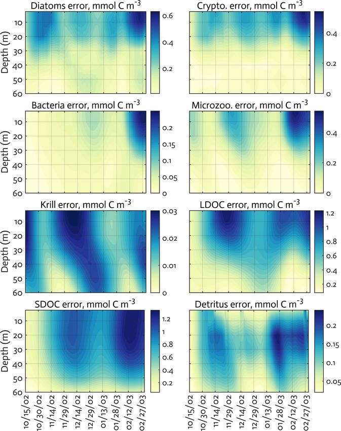
H. H. Kim et al.: WAP-1D-VAR v1.0: variational data assimilation model                                                               4941

Figure 1. The WAP-1D-VAR v1.0 model is forced by five different physical forcing, denoted as a horizontal row across the top of the
schematic of the ecosystem model. The ecosystem component incorporates 11 different prognostic state variables. Higher level and refractory
dissolved organic matter (RDOM) are represented implicitly.

that the entire LDOM pool is available but only a limited               and PO4 for inorganic (macro)nutrient compartments, but
portion of the SDOM is available for bacterial utilization              there is not a separate Fe model compartment or Fe uptake
to account for lower lability of SDOM. Refractory DOM                   processes, given that even during the peak of the blooms
(RDOM) is not explicitly modeled due to its much longer                 iron is still measurable and iron limitation is absent or oc-
turnover time than labile and semi-labile pools, but some               curs only minimally and seasonally in the nearshore Palmer
mass flows are included to RDOM from other prognostic                   Station area (Carvalho et al., 2016; Sherrell et al., 2018).
model compartments, such as bacteria, krill, and SDOM, to
account for loss terms for those state variables. Detritus rep-         2.2   Model equations
resents an average particulate organic matter (POM) pool af-
ter removing living phytoplankton and bacterial biomass, and            Here, we demonstrate key model processes that are either
sinking of the detritus pool contributes to particle export flux.       based on the existing schemes or built as new schemes for the
The WAP-1D-VAR model explicitly simulates NO3 , NH4 ,                   coastal WAP region. The original model schemes are detailed
                                                                        in Supplementary Material of Luo et al. (2010). The WAP-

https://doi.org/10.5194/gmd-14-4939-2021                                                   Geosci. Model Dev., 14, 4939–4975, 2021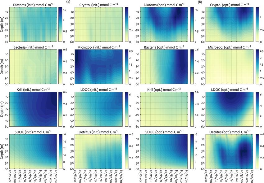
4942                                             H. H. Kim et al.: WAP-1D-VAR v1.0: variational data assimilation model

1D-VAR v1.0 model simulates biological–physical model            completely ceases when the phytoplankton cellular quota
processes for a 1-D vertical water column, solving numeri-       reaches their maximum allowable ratios and is additionally
cally for a discretized version of the time rate of change for   limited by the ambient NO3 and NH4 concentrations with a
each model state variable. For a generic tracer variable C,      Monod function (Eqs. A11–A12 and A55–A56). NH4 inhi-
the time rate of change equation takes the form (Glover et       bition on NO3 uptake of phytoplankton is modeled by as-
al., 2011)                                                       signing lower k NH4 compared to k NO3 (Table 1). The inhi-
∂C      ∂            ∂

                            ∂C
                                                                bition term does not exist for PO4 . The uptake scheme is
      = (wC) +           Kz      + JC ,                    (1)   similar for PO4 (Eqs. A14 and A58), but PO4 can be con-
 ∂t     ∂z          ∂z      ∂z                                   sumed in great excess of current needs (Armstrong, 2006).
where z is the depth, w is the vertical velocity (the sum of     Such luxury uptake is modeled by assigning smaller maxi-
water motion and gravitational particle sinking), Kz is the      mum and minimum P quota, which acts to alleviate P limita-
turbulent eddy diffusivity, and JC is the biological and bio-    tion. The maximum photosynthesis rate decreases when the
geochemical net source and sink term for C (Appendix A           phytoplankton cellular quota is lower than their reference ra-
Equations; Eqs. A42–A45, A82–A85, A138–A140, A164–               tio and approaches zero near their minimum ratio (Eqs. A7
A166, A193–A195, A199–A201, A205–A210, and A212–                 and A51). The Chl production decreases with lowering pho-
A214). The physical advection and mixing terms are dis-          tosynthetic active radiation (PAR) and completely ceases in
cussed below in Sect. 2.3 and applied sequentially follow-       dark (Eqs. A15 and A59). Phytoplankton release LDOM via
ing the computation of the biological and biogeochemical         passive diffusion of the low molecular weights DOM (e.g.,
terms JC using a constant time step of 1 h. The contributions    neutral sugars and dissolved free amino acids) with the same
of the source sink terms JC to the full time rate of change      cellular elemental ratio as that of phytoplankton (Fogg, 1966,
equations are constructed as a series of coupled ordinary dif-   Bjørnsen, 1988, Biddanda and Benner, 1997; Eqs. A17–A19
ferential equations, detailed in Appendix A (Sects. A1–A9),      and A61–A63). Phytoplankton also release L- and SDOM
and solved using a second-order Runge–Kutta numerical in-        actively, in the form of carbohydrate, as 75 % of the labile
tegration scheme. The WAP-1D-VAR model simulates the             (Eqs. A20, A24, A64, and A68) and 25 % of the semi-labile
dynamics of C, N, and P, but here we only focus on the pre-      pools (Eqs. A21, A27, A65, and A71). This active DOM
sentation of the model C dynamics. The cellular molar (e.g.,     production enables phytoplankton to adjust their stoichiom-
N/C, P/C) quota parameter values of most state variables are     etry to approach their reference ratio. If cellular organic C
fixed (Table 1) and not submitted to the optimization and data   is in excess, DOC is released on a timescale of 2 d, and if
assimilation procedure. To first order, most model physiolog-    excess nitrogen (phosphorus), DON (DOP) is released on
ical processes are affected by water temperature, including      a timescale of 8 d (Eqs. A22–A23 and A66–A67). Diatoms
the maximum growth rates of phytoplankton, bacteria, and         are grazed by both microzooplankton and krill (Eqs. A34–
zooplankton and basal respiration rates of bacteria and zoo-     A41), while cryptophytes are only grazed by microzooplank-
plankton. The Arrhenius function is implemented to change        ton (Eqs. A78–A81). Microzooplankton grazing functions
these physiological rates as a function of water temperature     are altered by assigning grazing limitation terms () to pro-
(Eq. A1).                                                        vide a limit on diatom grazing and route more cryptophytes
   The net change of phytoplankton (both diatoms and cryp-       to microzooplankton (Eqs. A34 and A78), based on initial
tophytes) C biomass is driven by gross growth, DOC excre-        modeling attempts where elevated diatom Chl was not simu-
tion, particulate organic carbon (POC) production via aggre-     lated due to their much stronger removal by microzooplank-
gation, respiration, and grazing (Eqs. A42 and A82), the net     ton than cryptophytes. In principle, optimization should be
change of their N and P biomass by gross growth, dissolved       able to capture the elevated diatom Chl by adjusting free
organic nitrogen (phosphorus) excretion, particulate organic     parameters unless (1) the right parameters are not adjusted
nitrogen (phosphorus) production, and grazing (Eqs. A43–         and/or the baseline (non-optimized) parameters need signif-
A44 and A83–A84). The net change of their chlorophyll            icant adjusting, and/or (2) the model equations are not ade-
a (Chl a) by gross growth, DOM excretion, and grazing            quate even with the optimized parameters. In our initial mod-
(Eqs. A45 and A85). The WAP-1D-VAR model adapts a                eling attempts, the model failed to simulate the elevated di-
phytoplankton growth scheme with flexible stoichiometry, in      atom Chl with varying sets of the model initial parameter val-
which phytoplankton cells are allowed to accumulate and          ues assigned to decouple diatoms from their grazers. Thus,
store more nutrients under light stress (Bertilsson et al.,      grazing limitation terms () are instead assigned to limit mi-
2003; Droop, 1974, 1983; McCarthy, 1980). The phytoplank-        crozooplankton grazing on diatoms for modeling purposes,
ton C growth rate is limited by their cellular nutrient quota    the implementation of which is not strictly based on the eco-
(Eqs. A2–A3 and A46–A47). Modified from Geider et al.            logical evidence of prey switching or of zooplankton mortal-
(1998), phytoplankton nitrogen uptake decreases when their       ity thresholds.
cellular N/C quota is higher than their reference (Redfield)        The net change of bacterial biomass is driven by their
ratio but not limited when lower than their reference ratio      gross growth (via L- and SDOM uptake; Eqs. A97–A99,
(Eqs. A5, A9, A49, and A53). The nitrogen consumption            A100–A101, and A106–A107), respiration (Eq. A110), S-

Geosci. Model Dev., 14, 4939–4975, 2021                                          https://doi.org/10.5194/gmd-14-4939-2021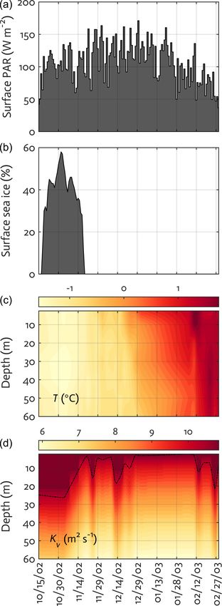
H. H. Kim et al.: WAP-1D-VAR v1.0: variational data assimilation model                                                                  4943

Table 1. Summary of the model parameter symbol and definition, initial parameter values (p0 ) and optimized values (pf ) for optimizable
parameters, the cost function gradient with regard to the optimized parameter (∂J /∂p), and prescribed values for fixed model parameters
over the course of simulations. The parameter with “n/a” in the parentheses is an optimized parameter with a large relative uncertainty, while
the parameter with values in the parentheses is a constrained parameter (optimized with a low relative uncertainty) with its upper and lower
bounds. The uncertainties for these upper and lower bounds are calculated as pf × e±σf , where pf is the value of the constrained parameter
and σf is the square roots of diagonal elements of the inverse of the Hessian matrix. The cost function gradient with regard to the optimized
parameter (∂J /∂p) after data assimilation is defined as 1J /e1p where e1p ≈ 1p for an infinitely small 1p.

 Model parameter symbol and definition (optimizable)                                             p0                    pf            ∂J /∂p
 AE , Arrhenius parameter for temperature function                                         4000.00                     –            −1.15
 µDA , diatom C-specific maximum growth rate, d−1                                              2.00     0.77 (0.68–0.88)     −5.53 × 10⁻⁵
 µCR , crypto. C-specific maximum growth rate, d−1                                             1.00     0.72 (0.61–0.85)      2.51 × 10⁻⁴
 αDA , initial slope of P–I curve of diatoms, mol C (g Chl)−1 d−1 (W m−2 )−1                   0.30     0.13 (0.10–0.19)     −1.55 × 10⁻⁴
 αCR , initial slope of P–I curve of crypto., mol C (g Chl)−1 d−1 (W m−2 )−1                   0.20    3.89 × 10⁻² (n/a)              0.45
 βDA , light inhibition parameter for diatom photosynthesis (W m−2 )−1                 5.00 × 10⁻³                     –            −1.10
 βCR , light inhibition parameter for crypto. photosynthesis (W m−2 )−1                5.00 × 10⁻³                     –              0.32
  N
 vREF,DA  , maximum N uptake rate per diatom C biomass, mol N (mol C)−1 d−1                    0.50                    –     −5.13 × 10⁻²
  N
 vREF,CR  , maximum N uptake rate per crypto. C biomass, mol N (mol C)−1 d−1                   0.30                    –     −3.07 × 10⁻²
   NH
 kDA 4 , NH4 half-saturation concentration for diatom uptake, mmol m−3                          0.10                    –              0.29
   NH
 kCR 4 , NH4 half-saturation concentration for crypto. uptake, mmol m−3                         0.10                    –              0.14
   NO
 kDA 3 , NO3 half-saturation concentration for diatom uptake, mmol m−3                          1.00                    –            −0.29
   NO
 kCR 3 , NO3 half-saturation concentration for crypto. uptake, mmol m−3                         0.60                    –            −0.14
   P
 vREF,DA  , maximum P uptake rate per diatom C biomass, mol P (mol C)−1 d−1                     0.03                    –             0.32
   P
 vREF,CR , maximum P uptake rate per crypto. C biomass, mol P (mol C)−1 d−1                     0.03                    –             0.15
   PO
 kDA4 , PO4 half-saturation concentration for diatom uptake, mmol m−3                           0.05                    –    −9.93 × 10⁻³
   PO
 kCR4 , PO4 half-saturation concentration for crypto. uptake, mmol m−3                         0.04                     –    −3.68 × 10⁻³
 ζ NO3 , C requirement (respiration) to assimilate NO3 , mol C (mol N)−1                       2.00                     –           −1.42
 Θ, maximum Chl/N ratio, g Chl a (mol N)−1                                                     2.90      2.27 (1.82–2.82)     5.95 × 10⁻⁵
 exPSV,DA , diatom passive excretion rate per biomass, d−1                                     0.05                     –             0.86
 exPSV,CR , crypto. passive excretion rate per biomass, d−1                                    0.05                     –             2.17
 exACT,DA , diatom active excretion rate per growth rate, d−1                                  0.05                     –     2.26 × 10⁻²
 exACT,CR , crypto. active excretion rate per growth rate, d−1                                 0.05                     –     4.06 × 10⁻³
 pomDA , POM production rate by diatom aggregation, (mmol C m−3 )−1 d−1                        0.04                     –             1.99
 pomCR , POM production rate by crypto. aggregation, (mmol C m−3 )−1 d−1                       0.03                     –             0.61
 k DOC , DOC half-saturation concentration for bacterial uptake, mmol C m−3                    0.65                     –             1.00
 rSDOM , parameter controlling SDOM lability                                           5.00 × 10⁻³                      –           −0.64
 µBAC , maximum bacterial growth rate, d−1                                                     2.00      1.06 (0.93–1.20)     1.54 × 10⁻⁴
 bR,BAC , parameter control bacterial active respiration rate vs. production,          1.50 × 10⁻²                      –     9.60 × 10⁻²
 (mmol C m−3 d−1 )−1
 exADJ,BAC , bacterial extra SDOC excretion rate, d−1                                          2.00                     –             0.00
 remiBAC , bacterial nutrient regeneration rate, d−1                                           6.00                     –           −0.11
 exREFR,BAC , bacterial RDOC production rate, d−1                                      1.70 × 10⁻²                      –             2.77
 fS , bacterial selection strength on SDOM                                                     0.25                     –    −5.18 × 10⁻³
  B , bacterial basal respiration rate, d−1
 rBAC                                                                                  1.27 × 10⁻²                      –             0.40
  A
 rmin,BAC  , bacterial minimum active respiration rate, d−1                            3.50 × 10⁻²                      –    −4.37 × 10⁻³
  A
 rmax,BAC , bacterial maximum active respiration rate, d−1                                     0.58      0.80 (0.77–0.84)    −6.59 × 10⁻⁴
 mortBAC , bacterial mortality rate, d−1                                                       0.02                     –             3.10
 µMZ , microzoo. C-specific maximum growth rate, d−1                                           1.00      1.18 (1.10–1.26)    −7.41 × 10⁻⁴
 gDA , diatom half-saturation concentration in microzoo. grazing, mmol C m−3                   1.00                     –             1.85
   0 , diatom half-saturation concentration in krill grazing, mmol C m−3
 gDA                                                                                           1.00                     –           −1.15

https://doi.org/10.5194/gmd-14-4939-2021                                                     Geosci. Model Dev., 14, 4939–4975, 2021
4944                                                     H. H. Kim et al.: WAP-1D-VAR v1.0: variational data assimilation model

Table 1. Continued.

  Model parameter symbol and definition (optimizable)                                          p0                  pf          ∂J /∂p
  gCR , crypto. half-saturation concentration in microzoo. grazing, mmol C m−3                1.00                   –            1.32
  gBAC , bacterial half-saturation concentration in microzoo. grazing, mmol C m−3             0.55   0.81 (0.64–1.03)     3.75 × 10⁻⁵
  exMZ , total DOM excretion rate per microzoo. gross growth, d−1                             0.15                   –            0.52
  fex,MZ , fraction of LDOC of total microzoo. DOC excretion                                  0.75                   –          −0.37
   B , microzoo. basal respiration rate, d−1
  rMZ                                                                                         0.01                   –    3.92 × 10⁻²
   A , microzoo. active respiration rate, d−1
  rMZ                                                                                         0.42                   –          −0.63
  exADJ,MZ , microzoo. extra SDOM excretion rate, d−1                                         2.00                   –            0.00
  remiMZ , microzoo. nutrient regeneration rate, d−1                                          4.68                   –    2.93 × 10⁻³
  pomMZ , POM production rate per microzoo. gross growth, d−1                         2.70 × 10⁻²                    –    2.87 × 10⁻²
  µKR , maximum krill C-specific growth rate, d−1                                             0.80   1.02 (0.97–1.07)     2.17 × 10⁻⁴
  gMZ , microzoo. half-saturation concentration in krill grazing, mmol C m−3                  1.00          0.15 (n/a)          −0.95
  exKR , total DOM excretion rate per krill gross growth, d−1                                 0.30                   –          −0.29
  fex,KR , fraction of labile DOC of total krill DOC excretion                                0.75                   –          −0.45
   B , krill basal respiration rate, d−1
  rKR                                                                                         0.03                   –          −0.50
   A , krill active respiration rate, d−1
  rKR                                                                                         0.30                   –          −1.08
  exADJ,KR , krill extra SDOM excretion rate, d−1                                             2.00                   –            0.00
  remiKR , krill nutrient regeneration rate, d−1                                              4.00                   –   −2.81 × 10⁻²
  pomKR , POM production rate per krill gross growth, d−1                                     0.15                   –          −0.38
  exREFR,KR , krill RDOC production rate, d−1                                                 0.02                   –   −6.43 × 10⁻²
  remvKR , krill removal rate by higher trophic levels, (mmol C m−3 )−1 d−1                   0.10          0.43 (n/a)            0.86
  fKR , fraction of SDOM production by krill                                                  0.10                   –    5.11 × 10⁻²
  fPOM,HZ , fraction of POM production by higher trophic level                                0.20                   –    4.86 × 10⁻²
  exREFR,SDOM , conversion rate of SDOM to RDOM, d−1                                  9.00 × 10⁻⁴                    –   −5.17 × 10⁻²
    C
  qN,RDOM      , RDOM N/C ratio, mol N (mol C)−1                                              0.05                   –          −0.10
    C
  qP,RDOM , RDOM P/C ratio, mol P (mol C)−1                                           6.50 × 10⁻⁴                    –    4.70 × 10⁻³
    C
  qN,POM     , N/C ratio for POM production by microzoo. and krill, mol N (mol C)−1           0.12                   –            0.12
    C
  qP,POM , P/C ratio for POM production by microzoo. and krill, mol P (mol C)−1       4.50 × 10⁻³                    –    6.24 × 10⁻²
  rntrf , nitrification rate (NH4 to NO3 ), d−1                                       7.60 × 10⁻²                    –   −3.74 × 10⁻²
  prfN , preference for dissolving N content in POM                                           1.10                   –            0.27
  prfP , preference for dissolving P content in POM                                           4.00                   –    1.67 × 10⁻⁴
  wnsv, detritus vertical sinking velocity, m d−1                                             5.00                   –            0.26
  diss, detrital dissolution rate, d−1                                                        0.14                   –            1.07
  Model parameter symbol and definition (fixed)                                                 p
  Tref , reference temperature in Arrhenius function, ◦ C                                   15.00
   C
  qN,MIN,DA      , minimum N/C ratio of diatoms                                       3.40 × 10⁻²
   C
  qN,MAX,DA        , maximum N/C ratio of diatoms                                             0.17
   C
  qN,RDF,DA      , reference (Redfield) N/C ratio of diatoms                                  0.15
   C
  qP,MIN,DA     , minimum P/C ratio of diatoms                                        1.90 × 10⁻³
   C
  qP,MAX,DA , maximum P/C ratio of diatoms                                            1.59 × 10⁻²
   C
  qP,RDF,DA     , reference (Redfield) P/C ratio of diatoms                           9.40 × 10⁻³
   C
  qN,MIN,CR      , minimum N/C ratio of crypto.                                       3.40 × 10⁻²
   C
  qN,MAX,CR       , maximum N/C ratio of crypto.                                              0.17
   C
  qN,RDF,CR , reference (Redfield) N/C ratio of crypto.                                       0.15
   C
  qP,MIN,CR     , minimum P/C ratio of crypto.                                        1.90 × 10⁻³
   C
  qP,MAX,CR      , maximum P/C ratio of crypto.                                       1.59 × 10⁻²
   C
  qP,RDF,CR , reference (Redfield) P/C ratio of crypto.                               9.40 × 10⁻³
   C
  qN,BAC    , reference (optimal) N/C ratio of bacteria                                       0.18
   C
  qP,BAC , reference (optimal) P/C ratio of bacteria                                          0.02

Geosci. Model Dev., 14, 4939–4975, 2021                                                  https://doi.org/10.5194/gmd-14-4939-2021
H. H. Kim et al.: WAP-1D-VAR v1.0: variational data assimilation model                                                           4945

Table 1. Continued.

       Model parameter symbol and definition (optimizable)                                                   p0    pf   ∂J /∂p
        C
       qN,MZ   , reference (optimal) N/C ratio of microzoo.                                                0.20
        C
       qP,MZ  , reference (optimal) P/C ratio of microzoo.                                         2.20 × 10⁻²
        C
       qN,KR   , reference (optimal) N/C ratio of krill                                                    0.20
        C , reference (optimal) P/C ratio of krill
       qP,KR                                                                                       8.00 × 10⁻³
       DA , grazing limit to the amount of diatoms available for microzoo. grazing, mmol C m−3    1.00 × 10⁻³
       CR , grazing limit to the amount of crypto. available for microzoo. grazing, mmol C m−3            2.95

and RDOM excretion (Eqs. A111–A113 and A120–A128),                       The net change of zooplankton (both microzooplankton
grazing (Eqs. A129–A131), and mortality due to viral attack           and krill) biomass is driven by their gross growth (via graz-
(Eqs. A132–A134). The WAP-1D-VAR model allows both                    ing on prey; Eqs. A143–A145 and A169–A171), L- and
L- and SDOM as the substrate sources for bacteria, and bac-           SDOM excretion (Eqs. A146–A154 and A172–A180), respi-
terial nutrient quota lets the lability of SDOM variable for          ration (Eqs. A157 and A183), POM production (Eqs. A158–
their selective utilization. All the LDOM pool is available,          A160 and A184–A186), and grazing (Eqs. A161–A163 and
while only a limited portion of the SDOM pool is allowed              A190–A192). Microzooplankton C growth is supported by
for bacterial utilization, the degree of which is controlled by       consuming cryptophytes and bacteria (Eqs. A143–A145),
an optimizable parameter controlling the relative utilization         while krill carbon growth is supported by consuming diatoms
of SDOM to LDOM, or SDOM lability (i.e., rSDOC , Eq. A96,             and microzooplankton (Eqs. A169–A171). Both zooplankton
Table 1). Bacterial C growth is determined by their cellular          compartments follow the Holling type-2 density-dependent
quota and available L- and SDOC concentration (Eqs. A97–              grazing function with a preferential selection on different
A98), in which the growth would be limited if bacterial cel-          prey species (Eqs. A34, A38, A78, A129, and A161). Both
lular nitrogen (phosphorus) quota is smaller than their ref-          zooplankton groups release a portion of the organic matter
erence ratios (Eqs. A93–A94). Bacteria take up LDOM in                that they ingest as DOM via sloppy feeding and excretion
the way that the ratio of labile dissolved organic nitrogen           (Eqs. A146–A148, A149–A151, A172–A174, and A175–
(LDON) (LDOP) to LDOC uptake is the same as the bulk                  A177) such that the ratio of the released DON (DOP) to
N/C (P/C) ratio of the LDOM (Eqs. A100 and A106). Bac-                LDOC is equivalent to the N/C (P/C) ratio of zooplank-
teria take up SDOM with higher N/P ratios to reflect that             ton. The amount of SDOC excretion is a function of the to-
SDOM with higher N/P ratios is more labile (Eq. A98).                 tal carbon growth (Eqs. A149 and A175), while the amount
The ratio of semi-labile dissolved organic nitrogen (SDON)            of SDON (SDOP) excretion is also a function of the zoo-
to SDOC uptake by bacteria would vary between the bulk                plankton cellular N/C (P/C) ratio relative to their reference
N/C of SDOM and the bacterial reference cellular quota                ratio (Eqs. A150–A151 and A176–A177). Zooplankton ad-
(Eqs. A101 and A107). Bacteria are modeled to either take up          just their body cellular quota by either releasing SDOM if
or release NH4 and PO4 to maintain their stable and consis-           carbon is in excess or by regenerating NH4 or PO4 if nitro-
tent stoichiometry (Kirchman, 2000). Bacteria take up NO3             gen or phosphorus is in excess (Eqs. A152–A156 and A178–
only if their cellular N/C ratio is smaller than their refer-         A182), similar to the bacterial scheme. Respiration is for-
ence ratio (i.e., when bacteria are short of nitrogen), in or-        mulated such that basal respiration is based on a portion of
der to reflect higher energetic cost of NO3 uptake than NH4 ,         zooplankton biomass, while active respiration is based on
but the amount of NO3 uptake is modeled to be no more                 a portion of their grazed C (Eqs. A157 and A183). Both
than 10 % of N-specific bulk L- and SDOM uptake, and the              zooplankton egest fecal matter as POM (Eqs. A158–A160
sum of NO3 and NH4 uptake is modeled to be no more than               and A184–A186), but only krill additionally excrete RDOM
N-specific bulk L- and SDOM uptake (Eqs. A102–A105).                  with N/C and P/C similar to bacteria (Eqs. A187–A189).
These limit the maximum NO3 uptake rate and set the inhibi-           Microzooplankton are grazed by krill (Eqs. A161–A163),
tion of NH4 uptake on NO3 uptake. Bacteria excrete RDOM               while krill are removed by implicit higher trophic levels
by transforming LDOM to RDOM (Eqs. A111–A113). Bac-                   (Eqs. A190–A192), similarly calculated as a bacterial mor-
teria also adjust their cellular stoichiometry by remineral-          tality term rather than as an explicit grazing process.
izing NH4 and PO4 if carbon is in short (i.e., N and P in                The net change of detritus is driven by POM production
excess; Eqs. A114–A115) and by excreting SDOC if car-                 by all phyto- and zooplankton compartments that is routed
bon is in excess (i.e., nitrogen and phosphorus are in short;         to detrital pool (Eqs. A30–A33, A74–A77, A158–A160, and
Eqs. A123–A128). Bacteria are grazed by microzooplankton              A184–A186) and its dissolution (Eqs. A196–A198). An op-
(Eqs. A129–A131), and a certain percentage of bacteria gets           timizable vertical sinking speed is assigned to detritus to de-
lost to LDOC pool due to viral attack (Eqs. A132–A134).               rive particle export flux (i.e., particle export flux is equal to

https://doi.org/10.5194/gmd-14-4939-2021                                                 Geosci. Model Dev., 14, 4939–4975, 2021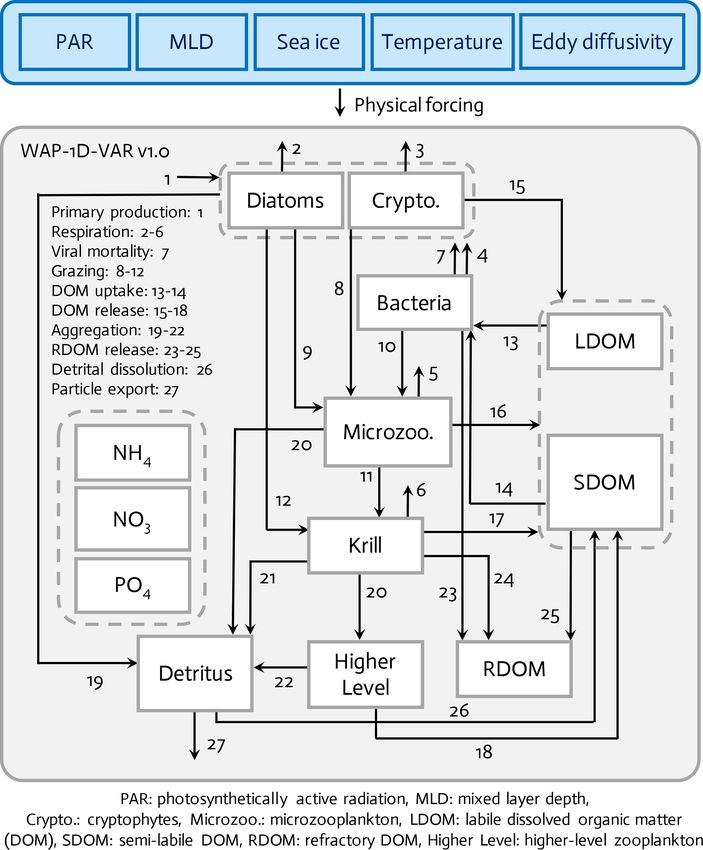
4946                                               H. H. Kim et al.: WAP-1D-VAR v1.0: variational data assimilation model

detrital concentration multiplied by particle sinking velocity,     calculated as follows:
wnsv, Table 1). The detritus that is lost due to dissolution
is incorporated to SDOM pool when it sinks (Eqs. A208–              PAR(z) = PAR0 × exp {−(kw + kc × CHL) × z} ,                   (3)
A210) before regenerated to inorganic nutrients, rather than        where z is depth (m), PAR0 is PAR level at sea sur-
directly regenerated from as the particulate form. The net          face (W m−2 ), kw is the attenuation coefficient for sea-
change of LDOM is driven by LDOM excretion by all phyto-            water (m−1 ), kc is the attenuation coefficient for Chl
and zooplankton compartments (Eqs. A17–A20, A61–A64,                ((mg Chl)−1 m2 ), and CHL is the Chl concentration
A146–A148, and A172–A174) and the amount of bacterial               (mg Chl m−3 ).
mortality that is incorporated to LDOM due to viral attack             Sea-ice conditions in the coastal WAP do not necessar-
(Eqs. A132–A134) and its uptake by bacteria (Eq. A97).              ily represent solely local temperature and climate condi-
The net change of SDOM is driven by SDOM excretion by               tions, given that sea ice can be impacted by temperature,
all organisms (Eqs. A21–A23, A65–A67, A149–A154, and                mixed layer, heat fluxes, regional winds, and other physi-
A175–A180), the amount of detrital dissolution (Eqs. A196–          cal processes (Saenz et al., in review). We implement a sea-
A198), uptake by bacteria (Eqs. A98–A99), and conver-               ice model scheme to account for light transmission through
sion to RDOM pool (Eqs. A202–A204). The conversion of               sea ice (5 % of incident irradiance, as a typical transmit-
SDOM to RDOM pool is a function of the stoichiometry                tance value used in the Community Earth System Model)
of SDOM, in which the conversion process is slower for              and non-linearities in the photosynthesis–irradiance (P–I) re-
higher N/C and P/C of SDOM, to reflect that nitrogen- and           sponse under partial ice concentration (Long et al., 2015) us-
phosphorus-enriched SDOM is more likely labile. A cer-              ing percent daily sea-ice concentration data (GSFC Bootstrap
tain percentage of NH4 is converted to NO3 on a daily ba-           versions 2/3, derived from SMMR/SSMI satellite tempera-
sis to represent a simple nitrification process in the model        ture brightness data binned into 25 by 25 km grid cells). In
(Eq. A211).                                                         many previous models, the light-limitation term L(I ) is cal-
2.3    Physical forcing                                             culated as a function of mean irradiance I averaged over both
                                                                    ice-covered and open-water conditions, so L(I ); instead, we
The WAP-1D-VAR v1.0 model is forced by mixed layer                  compute the mean of light-limitation term (L(I )) as a func-
depth (MLD), PAR at the ocean surface, sea-ice concentra-           tion of fractional sea ice and open-water and incident irradi-
tion, water-column temperature, vertical velocity, and verti-       ance:
cal eddy diffusivity, at a temporal resolution of 1 d. Temper-
                                                                    L(I ) = P C PMAX
                                                                                 C
                                                                                         = 1 − exp(−I /Ik )                    (4)
ature, sea ice, and vertical eddy diffusivity are set up at every
vertical grid (depth) point.                                        L(I ) = fi × L(Ii ) + fo × L(Io ),                             (5)
   MLD is determined based on a finite difference den-                                                                             C
sity criterion with a threshold value of 1σθ = 0.03 kg m−3          where P C is the C-specific photosynthetic rate (d−1 ), PMAX
(Montégut et al., 2004) after calculating potential density         is the maximum photosynthetic rate (d−1 ), Ik is the parame-
of water mass from temperature and salinity conductivity–           ter describing the light-saturation behavior of the P–I curve
temperature–depth (CTD) observations. Vertical velocity, w,         (W m−2 ), Io is the open-water irradiance, Ii is the under-ice
is assigned as zero because it is very weak in the surface wa-      irradiance (i.e., Ii = 0.05 × Io ), fi is the fraction of area cov-
ters of the study site and materials are transported vertically     ered with sea ice, and fo is the fraction of open water (i.e.,
mostly by diffusion. The vertical eddy diffusivity scheme           fo = 1 − fi ).
treats the rapid vertical mixing in the surface boundary layer
                                                                    2.4   Variational data assimilation
by homogenizing model state variables instantaneously in
the mixed layer (i.e., by averaging at every time step). Thus,      The WAP-1D-VAR v1.0 model is equipped with a built-
Kz value above MLD is not required, and only Kz below               in data assimilation scheme based on a variational adjoint
MLD is calculated as follows:                                       method (Lawson et al., 1995). This method generates optimal
Kz (z) = Kz0 × exp {−α × (z − MLD)} ,                        (2)    model solutions that minimize the difference between model
                                                                    results and observations by objectively optimizing model pa-
where z is depth (m) below MLD and Kz0 is the vertical              rameter values (Friedrichs, 2001; Spitz et al., 2001; Ward et
eddy diffusivity at the bottom of the mixed layer (1.1 ×            al., 2010). In detail, the assimilation scheme (Fig. 2) consists
10−4 m2 s−1 ) (Klinck, 1998; Smith et al., 1999), and α is 0.01     of four steps (Glover et al., 2011): (1) starting with initial
(m−1 ).                                                             values of the model parameters (see below), the model is in-
   Daily surface downward solar radiation flux (National            tegrated forward in time from specified initial conditions to
Centers for Environmental Prediction reanalysis daily aver-         calculate the difference between the model simulation and
ages) is used to calculate sea surface PAR. PAR is estimated        the field data, or the model–observation misfit (i.e., cost func-
as 46 % of the total solar radiation (Pinker and Laszlo, 1992,      tion; Sect. 2.5, Eq. 6); (2) an adjoint model constructed us-
Kirk, 1994). The attenuation of PAR as a function of depth is       ing the Tangent linear and Adjoint Model Compiler (TAPE-

Geosci. Model Dev., 14, 4939–4975, 2021                                              https://doi.org/10.5194/gmd-14-4939-2021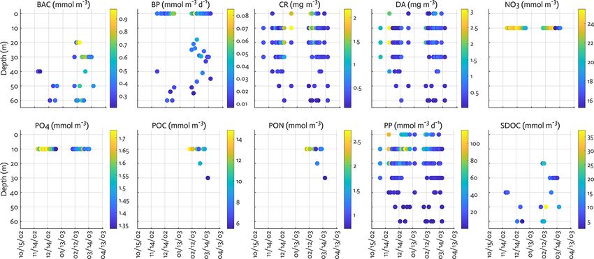
H. H. Kim et al.: WAP-1D-VAR v1.0: variational data assimilation model                                                                4947

                                                                          These include αDA (initial slope of photosynthesis vs. irra-
                                                                          diance curve of diatoms, mol C (g Chl a)−1 d−1 (W m−2 )−1 ),
                                                                          αCR (initial slope of photosynthesis vs. irradiance curve of
                                                                          cryptophytes, mol C (g Chl a)−1 d−1 (W m−2 )−1 ), Θ (maxi-
                                                                          mum Chl/N ratio, g Chl a (mol N)−1 ), µBAC (maximum bac-
                                                                                                      A
                                                                          terial growth rate, d−1 ), rmax,BAC  (maximum bacterial active
                                                                                               −1
                                                                          respiration rate, d ), gBAC (half-saturation density of bacte-
                                                                          ria in microzooplankton grazing, mmol C m−3 ), µMZ (max-
                                                                          imum microzooplankton growth rate, d−1 ), µKR (maximum
                                                                          krill growth rate, d−1 ), and remvKR (krill removal rate by
                                                                          higher trophic levels (mmol C m−3 )−1 d−1 ; Table 1).
                                                                             When computed at the minimum of the cost function
                                                                          value, the inverse of the Hessian matrix provides the uncer-
Figure 2. A variational adjoint scheme is employed for the pa-            tainties of optimized parameters, cross-correlations among
rameter optimization and data assimilation processes (adapted from        parameters, and sensitivities of the total cost function to each
Glover et al., 2011). Gradient: the sensitivity of the total cost func-   parameter (Matear, 1996; Tziperman and Thacker, 1989).
tion with respect to model parameter from optimization.
                                                                          High off-diagonal values in the inversed Hessian matrix in-
                                                                          dicate highly cross-correlated model parameters, so one of
                                                                          the highly cross-correlated parameters is removed from the
NADE) is integrated backward in time to compute the gra-                  optimization. The square root of a diagonal element in the
dients of the total cost with respect to the model parame-                inversed Hessian matrix is the logarithm of the relative uncer-
ters; (3) the computed gradients are then passed to a limited-            tainty (σf ) of the corresponding optimized parameter. The ab-
memory quasi-Newton optimization software M1QN3 3.1                       solute uncertainty of the constrained parameter is calculated
(Gilbert and Lemaréchal, 1989) to determine the direction                 as pf × e±σf where pf is the value of the optimized parame-
and optimal step size by which the selected model parame-                 ter (Table 1). If optimized to ecologically unrealistic values,
ters (see below) need to be modified in order to reduce the               parameters are kept back to their respective initial values and
total cost; and (4) a new forward-in-time simulation is con-              removed from the next optimization cycle. Optimized param-
ducted using the new set of modified (optimized) parameter                eters with σf larger than 50 % are updated but removed from
values. These four-step procedures are conducted in an iter-              the next optimization cycle (i.e., defined as “optimized” pa-
ative manner until the preset convergence criteria (i.e., low             rameters), while optimized parameters with σf smaller than
gradients of the total cost function with respect to optimized            50 % are updated and kept for the next optimization cycle
parameters and positive eigenvalues of the Hessian matrix)                (i.e., defined as “constrained parameters”). Constrained pa-
are satisfied to ensure that the optimized parameters converge            rameters are reported with the uncertainties, while optimized
and the total cost function reaches a local minimum.                      parameters are reported without the uncertainties (Table 1)
   Initial values of the model parameters (total of 72 free or            because both changed parameters consist of an optimized
optimizable parameters, Table 1) are assigned based on lit-               model parameter set, but the parameters reported with the un-
erature values (Caron et al., 2000, Luo et al., 2010, Garzio              certainty ranges are the ones optimized with relatively small
et al., 2013) without examining the effects of the initial pa-            uncertainties and considered constrained. This way, a part of
rameter values on the model results prior to optimization.                the initial parameter subset forms a final optimized parameter
As is typical for many types of ecosystem models, a col-                  set. The gradients of the total cost function with respect to all
lection of what appear to be reasonable initial parameter es-             72 parameters are then evaluated, the parameters with large
timates can result in relatively poor overall system behav-               gradients (e.g., > 5) are re-submitted to optimization to fur-
ior because of system-level interactions of different model               ther reduce the total cost, the gradients are evaluated again,
components. In most marine ecosystem models, these ini-                   and these cycles repeat until the termination of optimization.
tial parameter values are subjectively and manually adjusted              Optimization terminates when the gradients are reasonably
to improve the simulation, and the simulations with the ini-              low (e.g., < 10−2 for constrained parameters, < 5 for op-
tial, unadjusted parameter values are rarely shown. However,              timized parameters, and < 10 for unoptimized parameters).
here with a more objective optimization approach that we                  This final optimized model parameter set forms the basis of
conduct, the initial and optimized solutions can be explic-               the results presented throughout this study (Sect. 4). Addi-
itly compared (Sect. 4). Optimization starts by submitting a              tionally, in order to assess the sensitivity of the model opti-
subset of the 72 free model parameters rather than submit-                mization results with regard to the initial parameter choice,
ting all of them at once. This initial parameter subset con-              we perturb by ±50 % a subset of the initial parameter values
sists of 10 different model parameters, the change of which               used in the reference (original) optimization experiments to
yields the largest decrease in the total cost function (i.e.,             form different initial parameter sets (a total of 15 sets consist-
which also happens to be usually one per each state variable).

https://doi.org/10.5194/gmd-14-4939-2021                                                     Geosci. Model Dev., 14, 4939–4975, 2021
4948 H. H. Kim et al.: WAP-1D-VAR v1.0: variational data assimilation model
ing of partially or fully perturbed 18 parameters, Tables B1– 3 Model experiments
2) and conduct new optimization experiments from each set
(Sect. 4.1). 3.1 Modeling framework
2.5 Cost function To examine the applicability of the WAP-1D-VAR v1.0
model to the coastal WAP region, we select a nearshore
To represent a misfit between observations and model out- Palmer LTER water-column time-series station, Station E
put, a total cost function is calculated as follows (Luo et al., (64.77◦ S, 64.05◦ W), as the modeling site that is ∼ 200 m
2010): deep and situated approximately 3 km south of Palmer Sta-
Nm tion and 6.5 km northeast of the head of Palmer Deep (Sher-
M
âm,n − am,n 2
X 1 X rell et al., 2018). Physical forcing (Fig. 3) and data types
J= , (6)
N
m=1 m n=1
σm assimilated are derived from roughly semi-weekly physical,
chemical, and biological profiles collected from small boat
where m and n represent assimilated data types and data via a profiling CTD and discrete water samples at Station E.
points, respectively, M and Nm are the total number of as- When weather and ice conditions permit, water-column sam-
similated data types and data points for data type m, respec- pling at the station has been conducted twice a week over the
tively, σm is the target error for data type m, am,n is obser- growth season. Seven upper-ocean layer depths (2.5, 10, 20,
vations, and âm,n is model output. Given the high biologi- 30, 40, 50, and 60 m) are chosen for the model vertical grids.
cal productivity of the WAP waters and the approximate log- The model depth can be extended to as deep as needed, but
normal distribution of many marine biological variables, the this study is focused to upper 60 m water column to fully take
base-10 logarithms of Chl and primary production (PP) are advantage of the large data availability. Also, conceptually,
used in the cost function calculation to capture phytoplankton the application of the 1-D model framework makes the most
dynamics (Campbell, 1995; Glover et al., 2018). The target sense for the upper water column dominated by local sea-
error is calculated for each data type as follows: sonal processes, and extension of the model into deeper wa-
ter well below the maximum seasonal mixed layer becomes
σm = am,n × CVm , (7) more problematic because of the growing importance of lat-
eral advective processes that are not well captured in the 1-
where am,n is the climatological mean (over the select nine
D model framework. The vertical structure of the water col-
growth seasons; see below) of the observations and CVm is
umn can be affected by growing sea ice due to reduced wind-
the averaged coefficient of variation (CV) of the observa-
driven turbulence and brine rejection during winter, but this
tions of each data type in the mixed layer (due to observa-
is what a prognostic, coupled ocean–ice 1-D model can offer
tional error and seasonal and interannual variations) calcu-
to simulate, not our diagnostic-forcing-based model that was
lated using all of the observational data over nine growth-
used in this study. Also, because our model simulates only
season periods between 2002–2003 and 2011–2012, except
the spring–summer growth season, the impact of winter sea
the 2007–2008 growth season due to its missing data. These
ice on ecosystem dynamics is less of a concern.
nine growth seasons are chosen, instead of the multi-decadal
Given the routine observations of Palmer LTER available
observations available from Palmer LTER (since 1991), due
over the growth season (October–March), we simulate one
to the relatively more complete data coverage in those sea-
example growth season with the most complete data cover-
sons. The standard deviations are used as target errors of the
age, from October 2002 to March 2003 (2002–2003 growth
log-converted data types. The CV of the log-converted data
season hereafter), instead of a series of different growth
type is estimated as the average of ±1 standard deviation in
seasons in a continuous manner. The example growth sea-
log space converted back into normal space (Doney et al.,
son simulations utilize this year’s specific observed physical
2003; Glover et al., 2018). Hereafter, we present the total cost
forcing fields and assimilated biological and biogeochemical
normalized by M (J equivalent to J /M hereafter) as it indi-
observations. Each Palmer LTER growth season should be
cates the model–observation misfit equivalent to a reduced
modeled to have its own unique optimized parameter set, as
chi-square estimate of model goodness of fit. We report the
well as initial conditions and physical forcing that together
normalized total cost J along with normalized costs of in-
determine the model solution for that year; however, only the
dividual data types throughout this study. J = 1 indicates a
2002–2003 growth season simulations are modeled in this
good fit, J
1 indicates a poor fit or underestimation of the
study for model analysis and evaluation.
error variance, and J
1 indicates an overfitting of the data,
fitting the noise, or overestimation of the error variance.
3.2 Initial and boundary conditions
Model initial conditions are prescribed 135 d before the
model start date for the growth season (15 October 2002)
on 1 June 2002. This 135 d spinup is conducted to mini-
Geosci. Model Dev., 14, 4939–4975, 2021 https://doi.org/10.5194/gmd-14-4939-2021H. H. Kim et al.: WAP-1D-VAR v1.0: variational data assimilation model 4949
in the optimization of the 2002–2003 growth season (i.e., cli-
matological model; using climatological physics and obser-
vations averaged over nine growth-season periods between
2002–2003 and 2011–2012 except the 2007–2008 growth
season due to its missing data). For the first climatologi-
cal model simulation, initial conditions are prepared by ad-
justing manually following literature values (e.g., Luo et
al., 2010). Due to strong interannual variability in the phy-
toplankton bloom phenology at Palmer Station, averaging
across all these 9 years does not reflect distinct seasonal phy-
toplankton peaks, leading to underestimated phytoplankton
values (not shown). To capture this non-linear aspect of the
coastal WAP system, we construct the climatological year
by applying a single time shift to all variables so that a sea-
sonal PP peak of each year lines up with an average date
of seasonal PP peaks from all years. Most biological initial
conditions on 1 June are close to zero given the lack of active
physiological processes in the very low light and the presence
of sea ice during wintertime before the model growth season
starts. All the data types are set to zero at the lower boundary
(bottom) except for NO3 , PO4 , SDOC, SDON, and SDOP in
which the climatological values at 65 m are used for lower
boundary values (25.9, 1.9, 6.5, 0.6, and 0.03 mmol m−3 , re-
spectively).
3.3 Assimilated data
We include the data types directly related to corresponding
model outputs, including a mix of ecosystem stocks or state
variables – NO3 , PO4 , Chl for diatoms and cryptophytes,
bacterial biomass, microzooplankton biomass, SDOC, POC,
and particulate organic nitrogen (PON), as well as carbon
flows among model stocks – bulk net PP and bacterial pro-
duction (BP). These data sets have been sampled semi-
weekly at Palmer Station E (64.77◦ S, 64.05◦ W), the same
location where our model is set up, and are available from
the Palmer LTER data website (see data availability). The
distinction between diatoms and cryptophytes is established
by assimilating phytoplankton taxonomic-specific Chl data
for diatoms and non-diatom species derived from a high-
performance liquid chromatography (HPLC) and CHEM-
TAX analysis (Schofield et al., 2017), but given cryptophytes
being the second dominant species in the water samples
Figure 3. Physical forcing used in the WAP-1D-VAR v1.0 model, at the study site, cryptophytes are assumed to represent all
including surface photosynthetically active radiation (PAR) (a), sea- non-diatom species for modeling purposes. Given that POC
ice concentration (b), water temperature (c), and vertical eddy dif- (PON) from bottle filtration may capture both living biomass
fusivity (d) overlaid with mixed layer depth (MLD; dashed line) in and detrital material, we adjust the observed POC (PON)
the modeled growth season of 2002–2003. by subtracting phytoplankton and bacterial C (N) biomass
to estimate the detrital pool, in order to only include non-
living particles to detrital pool. When phytoplankton or bac-
mize the impact of initial conditions on the model output terial biomass data are not available, we assign climatolog-
over the growth season. Initial conditions are prepared by ical (2002–2003 to 2011–2012) fractions of POC (PON) to
optimizing the full growth seasonal cycle forced by clima- detrital pool. Phytoplankton and bacterial biomass accounts
tological physics and assimilated with climatological obser- for 26 % of total POC and 29 % of total PON. In converting
vations and with the same bottom boundary conditions used Chl to phytoplankton carbon (nitrogen) biomass, the max-
https://doi.org/10.5194/gmd-14-4939-2021 Geosci. Model Dev., 14, 4939–4975, 20214950 H. H. Kim et al.: WAP-1D-VAR v1.0: variational data assimilation model
imum Chl/C (Chl/N) ratio submitted for optimization is observations and model output compared to the misfits ob-
used along with other reference ratios (Table 1). Microzoo- tained from the initial parameter values (Table 2). The opti-
plankton biomass data are not available for the full time se- mized model solution satisfied the preset convergence crite-
ries, so their data from grazing experiments at Palmer Sta- ria, with the low gradients of the total cost with respect to the
tion (Garzio et al., 2013) are assimilated to at least pro- optimized parameters and positive eigenvalues of the Hessian
vide constraints on bacterial and cryptophyte grazing pro- matrix. Notably, this was achieved by optimizing a subset of
cesses. However, due to the discrepancy in the timing and 12 (9 constrained and 3 optimized) parameters among the to-
location from model simulations of this study, the micro- tal of 72 optimizable parameters (Table 1, Sect. 4.2). To ex-
zooplankton model–observation misfits are not analyzed in amine the sensitivity of the optimized model solution to the
the present study. Krill biomass data are not assimilated due initial parameter choice, a series of new optimization exper-
to the strong patchiness of their distribution that may hin- iments (n = 15) was conducted with a varying subset of the
der proper model optimization. The vertical profiles of most initial parameter values perturbed by ±50 % of those used
of the data types are assimilated, whereas average NO3 and in the original optimization experiment (Table B1). These
PO4 concentrations in the mixed layer are assimilated due experiments showed that the optimized model results (i.e.,
to the difficulty of simulating depth-dependent nutrient con- the reference case; Table 1) were not sensitive to the initial
centrations and the fact that net PP is mostly determined choice of the parameters. The 15 different initial parame-
by surface nutrient concentrations (Luo et al., 2010). BP ter sets resulted in a range of initial model–observation mis-
(mmol C m−3 d−1 ) is derived from the 3 H-leucine incorpo- fits, some substantially larger than the reference case (14.25–
ration rate (pmol l−1 h−1 ) data using the conversion factor 28.24 vs. 14.85 for the reference case). However, the total
of 1.5 kg C (mol leucine)−1 incorporated (Ducklow, 2000). normalized optimized cost values of the 15 sensitivity exper-
Bacterial biomass (mmol C m−3 ) is estimated from bacte- iments (5.79–7.19) were similar to that of the reference case
rial abundance measured by flow cytometry with the con- of 6.42. In sensitivity experiment no. 12, the initial model–
version factor of 10 fg C cell−1 (Fukuda et al., 1998). SDOC observation misfit was ∼ 2 times larger than that of the ref-
is calculated by subtracting the background concentration erence case, and there was up to 76 % of the reduction in
(41.2 mmol m−3 for the modeling site) from total DOC con- the model–observational misfit (vs. 58 % of the reduction in
centration. the reference case; Table B1, Table 1). These results sug-
gest that no matter where in parameter space the optimiza-
3.4 Uncertainty analysis tion process starts from, the optimization scheme takes the
model cost function to similar local minima. Importantly, this
Uncertainties of the optimized parameters are computed was achieved by similar subsets of the optimized parameters:
from a finite difference approximation of the complete Hes- A
µDA , µCR , rmax,BAC , and µMZ were optimized in all cases,
sian matrix (i.e., second derivatives of the cost function with while αDA , αCR , Θ, µBAC , gCR , gDA 0 ,g
BAC , µKR , gMZ , and
respect to the model parameters) during the iterative op- remvKR were optimized except for a few cases (Table B1).
timization process (details in Sect. 2.4). We then conduct The uncertainties of the optimized parameters were also sim-
Monte Carlo experiments to calculate the impact of the op- ilar among different optimizations, with most of the relative
timized parameter uncertainties on the model results. We errors < 0.5. Constrained parameter values and their uncer-
first create an ensemble of parameter sets (n = 1000) by ran- tainty ranges averaged over the sensitivity experiments (Ta-
domly sampling values within the uncertainty ranges of the ble B2) were comparable to those in the original optimization
constrained parameters and then perform a model simulation experiments (Table 1).
using each parameter set. A total of 1000 Monte Carlo ex- Overall, there was a good model–data fit with the largely
periments were shown to be adequate from a series of tests decreased cost value for each data type after optimization
with different numbers of Monte Carlo sampling (n = 500– (Table 2). Optimization yielded Jf close to 1 for all data
2000), where standard deviations of model-simulated values types, compared to the initial model solution where three data
converged after > 1000 Monte Carlo sampling (not shown). types – diatom Chl, crypto Chl, and bacterial biomass – had
All uncertainty estimates are calculated following standard particularly poor model fits to observations and underesti-
error propagation rules and presented as ±1 standard devia- mated error variances (J
1). Compared to the initial (un-
tion in the study. optimized) model results, the average errors (εbias , Doney et
al., 2009; Stow et al., 2009) in the optimized model results in-
4 Results and discussion dicated that diatom Chl, cryptophyte Chl, bacterial biomass,
BP, and POC had reduced model biases, while NO3 , PO4 , PP,
4.1 Model skill assessment SDOC, and PON had increased model biases (for both pos-
itive and negative biases, defined as εbias > 0 and εbias < 0,
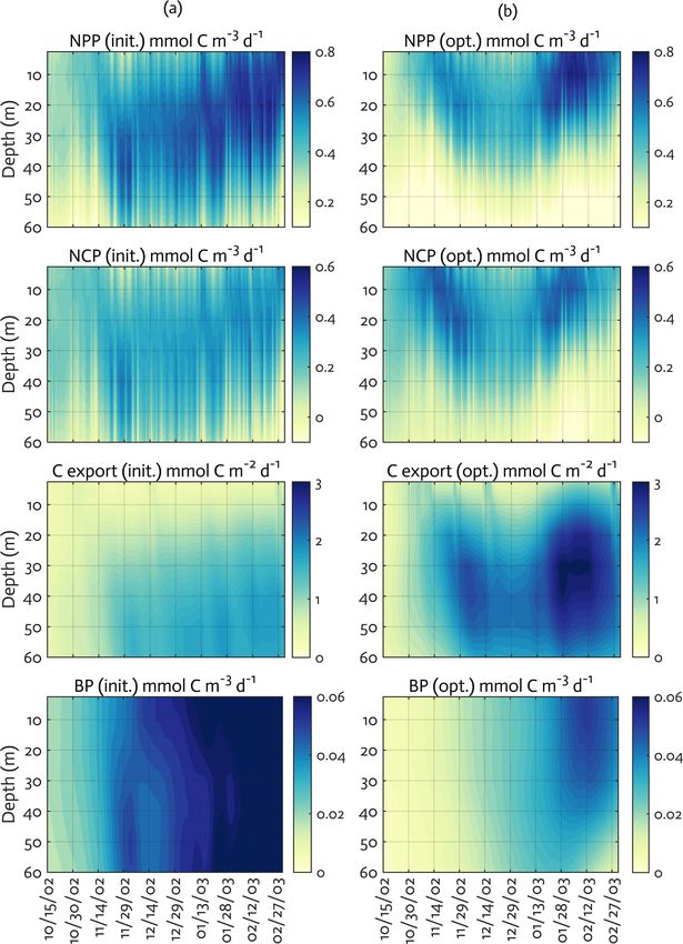
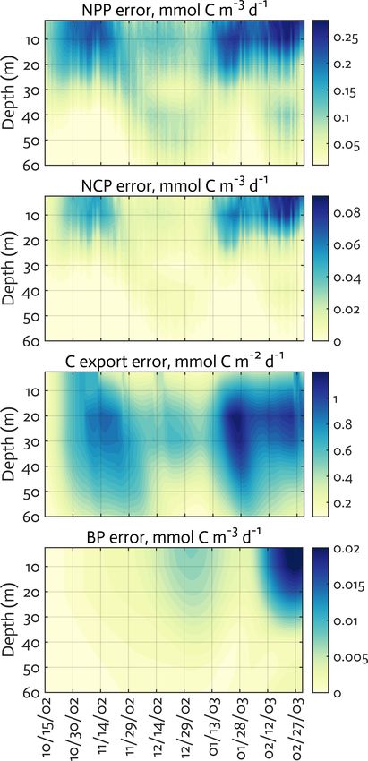
In the case of the example growth season (2002–2003) mod- for model overestimation and underestimation of the obser-
eled in this study, the iterative data assimilation–parameter vation, respectively). Optimization resulted in the negative
optimization procedure reduced by 58 % the misfits between model bias for PO4 , compared to the positive model bias in
Geosci. Model Dev., 14, 4939–4975, 2021 https://doi.org/10.5194/gmd-14-4939-2021You can also read