The zone of influence: matching sea level variability from coastal altimetry and tide gauges for vertical land motion estimation - mediaTUM
←
→
Page content transcription
If your browser does not render page correctly, please read the page content below
Ocean Sci., 17, 35–57, 2021
https://doi.org/10.5194/os-17-35-2021
© Author(s) 2021. This work is distributed under
the Creative Commons Attribution 4.0 License.

The zone of influence: matching sea level variability from coastal
altimetry and tide gauges for vertical land motion estimation
Julius Oelsmann, Marcello Passaro, Denise Dettmering, Christian Schwatke, Laura Sánchez, and Florian Seitz
Deutsches Geodätisches Forschungsinstitut der Technischen Universität München, Arcisstraße 21, 80333 Munich, Germany

Correspondence: Julius Oelsmann (julius.oelsmann@tum.de)

Received: 22 April 2020 – Discussion started: 27 May 2020
Revised: 27 August 2020 – Accepted: 26 October 2020 – Published: 12 January 2021

Abstract. Vertical land motion (VLM) at the coast is a sub-         1   Introduction
stantial contributor to relative sea level change. In this work,
we present a refined method for its determination, which            Coastal vertical land motion (VLM) significantly contributes
is based on the combination of absolute satellite altimetry         to relative sea level change (SLC). VLM is in many places
(SAT) sea level measurements and relative sea level changes         of the same order of magnitude (1–10 mm yr−1 ) as the sea
recorded by tide gauges (TGs). These measurements com-              level rise signal itself and displays significant spatial varia-
plement VLM estimates from the GNSS (Global Navigation              tions (Santamaría-Gómez et al., 2012). Consequently, VLM
Satellite System) by increasing their spatial coverage. Trend       affects coastal impacts of climate-sensitive processes and
estimates from the SAT and TG combination are particularly          can regionally account for large fractions of the observed
sensitive to the quality and resolution of applied altimetry        and projected coastal SLC signal (Wöppelmann and Mar-
data as well as to the coupling procedure of altimetry and          cos, 2016; Slangen et al., 2014). Thus, the accurate estima-
TGs. Hence, a multi-mission, dedicated coastal along-track          tion of VLM is vital, not only to disentangle climatic and
altimetry dataset is coupled with high-frequency TG mea-            geodynamic SLC signatures, but also to obtain more robust
surements at 58 stations. To improve the coupling proce-            estimates of past and future relative SLC and its associated
dure, a so-called “zone of influence” (ZOI) is defined, which       uncertainty (Church et al., 2013; Santamaría-Gómez et al.,
confines coherent zones of sea level variability on the basis       2017). In this work, we present a novel approach of VLM es-
of relative levels of comparability between TG and altime-          timation using coastal satellite altimetry, tide gauges and the
try observations. Selecting 20 % of the most representative         Global Navigation Satellite System (GNSS).
absolute sea level observations in a 300 km radius around              VLM is caused by the superimposition of natural pro-
the TGs results in the best VLM estimates in terms of ac-           cesses and anthropogenic influences in the Earth system and
curacy and uncertainty. At this threshold, VLMSAT-TG es-            operates on manifold spatial and temporal scales (Pugh and
timates have median formal uncertainties of 0.58 mm yr−1 .          Woodworth, 2014). Mechanisms such as the Glacial Isostatic
Validation against GNSS VLM estimates yields a root mean            Adjustment (GIA), the postglacial rebound of the Earth to
square (rms1VLM ) of VLMSAT-TG and VLMGNSS differences              changing ice and water load, cause distinct large-scale VLM,
of 1.28 mm yr−1 , demonstrating the level of accuracy of our        which can be assumed to be uniform on centennial timescales
approach. Compared to a reference 250 km radius selec-              (Peltier, 2004). Recent acceleration of land ice mass loss was
tion, the 300 km zone of influence improves trend accuracies        shown to additionally enhance deformation rates, posing new
by 15 % and uncertainties by 35 %. With increasing record           challenges for sea level studies due to its time-varying sig-
lengths, the spatial scales of the coherency in coastal sea level   nal (Riva et al., 2017). Surface mass changes are also caused
trends increase. Therefore, the relevance of the ZOI for im-        by terrestrial freshwater storage changes and can have small-
proving VLMSAT-TG accuracy decreases. Further individual            scale effects on VLM. Groundwater pumping, for instance,
zone of influence adaptations offer the prospect of bringing        contributes not only to local small-scale VLM and gravity
the accuracy of the estimates below 1 mm yr−1 .                     changes, but also modifies sea level rise in distant areas (e.g.,
                                                                    Wada et al., 2012; Veit and Conrad, 2016). Other small-scale

Published by Copernicus Publications on behalf of the European Geosciences Union.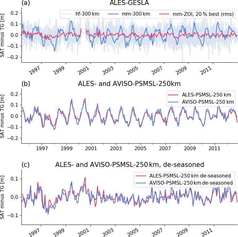
36                                                                                  J. Oelsmann et al.: The zone of influence

VLM effects such as erosion and tectonic movements can            (e.g., Bouin and Wöppelmann, 2010; Fenoglio et al., 2012;
be locally confined to several kilometers with more subtle,       Santamaría-Gómez et al., 2017). Wöppelmann and Marcos
not necessarily linear temporal behavior (Brooks et al., 2007;    (2016) identified comparably low formal errors of GNSS
Kolker et al., 2011; Poitevin et al., 2019). These and other      VLM rates (0.21 mm yr−1 ) when autocorrelation was taken
nonlinear processes at very short timescales are particularly     into account. Santamaría-Gómez et al. (2012) estimated an
challenging in the estimation of a linear rate of long-term       accuracy of 0.6 mm yr−1 of GNSS-based VLM (from at least
VLM from TGs, since they would appear as instabilities in         3 years of continuous data) by comparing 36 globally dis-
the record (similarly to a change in datum).                      tributed colocated GNSS velocity estimates. Thus, because
   In response to the substantial impact on relative sea level    of its considerable accuracy, vertical GNSS velocities fre-
and the large spectrum of VLM sources, several strategies         quently served as benchmark estimates for many sea level
have been developed to estimate VLM. The ability to capture       applications, e.g., for GIA model evaluation or local VLM
the diversity of VLM processes, however, strongly depends         corrections of TG records (Sánchez and Bosch, 2009; Sanli
on the method and geodetic technique used in the VLM es-          and Blewitt, 2001).
timation. Furthermore, the coverage and associated accuracy          For the latter use a necessary working hypothesis is that
of VLM estimates differ across the methods. Given that the        GNSS VLM represents the same movements as experienced
global absolute sea level trend during the altimeter era is       at the tide gauge (Wöppelmann and Marcos, 2016). Because
of the order of 3 mm yr−1 (3.1 ± 0.1 mm yr−1 from 1995 to         VLM is shown to potentially possess high spatial variabil-
2018 as reported in Cazenave et al., 2018), one prerequisite      ity even on small scales (tens of kilometers), GNSS stations
for VLM estimation is that the associated trend uncertainty       should ideally be very close to the tide gauge. This require-
should be at least 1 order of magnitude lower than this subtle    ment, however, reduces the number of available colocated
signal (Wöppelmann and Marcos, 2016). Hence, dense and            stations (130 GNSS stations within a 1 km range of GLOSS
accurate VLM estimates are required to complement mod-            – Global Sea Level Observing System – tide gauges; Wöp-
eled or measured rates of absolute sea level changes, which       pelmann et al., 2019) and thus confines the global coastal
is ultimately crucial for coastal planning. Improving the reli-   coverage to mostly Europe, Japan and North America.
ability of VLM estimates and their associated uncertainties          To extend the number of VLM estimates, several stud-
is thus one major concern of this study. In the following,        ies advanced the application of combining satellite altime-
we briefly contrast the three major approaches of deriving        try (SAT) and tide gauge (TG) observations (Cazenave et al.,
coastal VLM globally.                                             1999; Nerem and Mitchum, 2003; Kuo et al., 2004; Pfeffer
                                                                  and Allemand, 2016; Wöppelmann and Marcos, 2016; Klein-
1.1   Estimating coastal vertical land motions                    herenbrink et al., 2018). The principle of this approach is to
                                                                  subtract the absolute SLC gathered by the altimeter from rel-
The majority of global sea level studies have utilized geo-       ative SLC observations at the TG. Ideally, the differenced
dynamic GIA models to correct, for example, tide gauge            time series (SAT minus TG) yields the vertical displacement
records for secular land motion trends or to extrapolate fu-      of the TG with respect to the reference of the altimeter. The
ture relative SLC based on climate projections (e.g., Church      accuracy of this technique is, among numerous other factors,
and White, 2011; Hay et al., 1990; Carson et al., 2016).          strongly dependent on the stability of the altimeter measure-
GIA still represents the only long-term geological process        ment system. Major systematic errors stem from limitations
for which VLM can be modeled on a global scale. How-              in the realization of the reference frame and from limitations
ever, one caveat is that GIA VLM models were shown to             in the long-term stability of altimeter instruments and correc-
still be biased by imperfect assumptions of ice history and the   tions (e.g., Couhert et al., 2015; Wöppelmann and Marcos,
Earth’s structure (King et al., 2012), and they are thus model-   2016; Watson et al., 2015). Altimetry records can be affected
dependent (Jevrejeva et al., 2014). Another foreseeable dis-      by globally and regionally varying drifts, which were found
advantage is that the sole application of GIA models neglects     to be most pronounced on TOPEX altimeter side-A. The cal-
other sources of VLM (e.g., tectonics, erosion and anthro-        ibration of altimetry with TGs is influenced by the applied
pogenic impacts; Wöppelmann and Marcos, 2016). This led,          VLM correction (Watson et al., 2015). Conversely, SAT–TG
for instance, to discrepancies in estimated rates of histor-      VLM estimates are affected by the altimeter drift or by errors
ical global mean sea level (GMSL) change when compar-             originating from the intermission drift biases (or drifts with
ing model-based solutions against those using measurements        respect to the reference mission). Due to the availability of
from GNSS (Hamlington et al., 2016).                              global and continuous absolute sea level measurements, this
   For more than a decade, these direct geodetic estimates        method not only provides a complementary source to GNSS
(GNSS, such as GPS, GLONASS and GALILEO) have                     measurements, but also improves the geographical distribu-
been exploited to determine vertical velocities (Wöppelmann       tion of the data, as virtually every valid TG is usable.
et al., 2007; Snay et al., 2007; Mazzotti et al., 2008). GNSS        While all three sources of information, GIA models,
measurements denote the most precise source of VLM detec-         GNSS and “satellite altimetry minus tide gauge” (SAT–TG)
tion and are well established in local- to global-scale studies   techniques, have individual merits, their combined use is

Ocean Sci., 17, 35–57, 2021                                                            https://doi.org/10.5194/os-17-35-2021
J. Oelsmann et al.: The zone of influence                                                                                    37

valuable to further substantiate VLM estimates. GNSS ob-          stations of low comparability: with varying correlations be-
servations are necessary to validate both GIA models and the      tween 0.0 and 0.7, they obtained rms1VLM errors from 2.1
SAT–TG approach (Santamaría-Gómez et al., 2012; Wöp-              to 1.20 mm yr−1 (at 155 stations), which significantly im-
pelmann and Marcos, 2016; Kleinherenbrink et al., 2018).          proved WM16’s results. For a consistent set of stations, they
Recent studies have combined all three approaches to recon-       found a slight sensitivity of the rms1VLM to variations of
struct GMSL (Dangendorf et al., 2017) or to densify the esti-     the prescribed minimum correlation; however, they reported
mation of contemporary rates of vertical land motions (Pfef-      insignificant improvements of a few percent. Because they
fer et al., 2017) or relative sea level change (Hawkins et al.,   derived GNSS vertical velocities from the Nevada Geodetic
2019). Any advancement in these individual approaches             Laboratory (NGL) database by taking the median of avail-
therefore supports developments of the others and improves        able estimates within a 50 km range of the TG, they increased
the global assessment of coastal VLM estimates.                   the number at which VLMSAT-TG trends could be validated to
   In this study, we focus on enhancing the application of the    155.
SAT–TG difference for VLM detection. Our investigations              Based on Kleinherenbrink et al. (2018) and WM16, we
not only further develop the latest progress of the method,       identify two essential factors which are vital for the quality
but also gain a new perspective on sea level trend and un-        of trend estimation with the SAT–TG difference. Advance-
certainty characterization as well as quantification in coastal   ments with respect to both factors not only potentially led to
zones. The next section recapitulates the latest state of the     improved VLM estimates in Kleinherenbrink et al. (2018),
VLMSAT-TG estimation on which we base our innovations.            but also motivate further innovations.

1.2   Progress in VLM estimation by satellite altimetry            1. Data quality. In coastal regions the accuracy of altime-
      and tide gauge difference                                       try measurements is affected by the local departure of
                                                                      the radar signal from the known ocean response (due to
The combination of SAT and TG observations for VLM de-                inhomogeneities of the illuminated area) and by the in-
termination was steadily improved over the last 2 decades             accuracy of the standard routinely applied corrections
and is elaborated in the latest review by Wöppelmann and              and tidal models. Developments for the solution of both
Marcos (2016), hereinafter WM16. WM16 investigated per-               issues led to rapid improvements in the recent years
formances of different gridded and along-track altimetry              through, e.g., application of coastal retracking and ad-
products (e.g., AVISO – Archiving, Validation, and Inter-             vanced geophysical corrections (e.g., Cipollini et al.,
pretation of Satellite Oceanographic data; GSFC – God-                2017; Passaro et al., 2014; Fernandes et al., 2015).
dard Space Flight Center). They combined sea level anoma-             Dedicated coastal altimetry datasets (e.g., COASTALT,
lies (SLAs) as 1◦ radius averages with monthly mean TG                ALES, PISTACH) might thus outperform previously
records from PSMSL (Permanent Service for Mean Sea                    applied products (e.g., AVISO), which do not yet benefit
Level). Among all datasets, the gridded AVISO product re-             from these implementations.
vealed the best correlations and residuals between altime-
try and TG records. Using this dataset, WM16 also obtained         2. Data selection. Next to issues concerning data qual-
the most precise VLM estimates achieved, with median for-             ity, the second factor defining trend uncertainty is the
mal uncertainties of 0.8 mm yr−1 . Validation against GNSS-           sensitivity of VLMSAT-TG estimates to the spatial selec-
based trends from ULR5 (Université de La Rochelle, Insti-             tion of altimeter data in the vicinity of the TG. WM16
tut Géographique National analysis) at 113 colocated stations         showed that averaging SLA in a radius of 1◦ around the
resulted in an rms1VLM of 1.47 mm yr−1 of VLMSAT-TG and               TG resulted in higher correlations than using the best-
VLMGNSS trend differences, providing the highest accura-              correlated or the closest grid point to the TG. Klein-
cies among the datasets.                                              herenbrink et al. (2018) found a small influence of vari-
   Notwithstanding the weaker performance of the along-               ations of absolute correlation thresholds on the trend
track product (from GSFC) achieved in WM16, Kleinheren-               estimates. Therefore, considering the diversity of pro-
brink et al. (2018) made great progress in using along-track          cesses which drive coastal sea level variability, such
altimetry (TOPEX, Jason-1 and Jason-2 from the Radar Al-              as waves, winds or coastal and bathymetric properties,
timeter Database – RADS; Scharroo et al., 2012) to esti-              an advanced adaptation of the choice of altimetry SLA
mate VLM. Their approach aimed to overcome the spatial                might improve the representation of the signal captured
downsampling and associated loss of information in gridded            by the TG.
products such as AVISO. They also advanced the procedure
of combining altimetry and TG data. Instead of taking 1◦            These reasons motivate further improvements of both
averages around the TGs, they selected altimetry data ac-         components: the quality of the data and the practice of com-
cording to different absolute correlation thresholds and im-      bining altimetry and TG data. We aim to understand how
plemented correlation weighting of time series. Generally,        dedicated along-track coastal altimetry can outperform stan-
the thresholding strategy functioned as a filter to remove        dard gridded products. We also seek to generalize an optimal

https://doi.org/10.5194/os-17-35-2021                                                             Ocean Sci., 17, 35–57, 2021
38                                                                                        J. Oelsmann et al.: The zone of influence

Table 1. Applied models and geophysical corrections for estimating sea level anomalies.

                                Parameter                   Model            Reference
                                Range and sea state bias    ALES             (Passaro et al., 2014)
                                Inverse barometer           DAC-ERA          (Carrère et al., 2016)
                                Wet troposphere             GPD+             (Fernandes et al., 2015)
                                Dry troposphere             VMF3             (Landskron and Böhm, 2018)
                                Ionosphere                  NIC09            (Scharroo and Smith, 2010)
                                Ocean and load tide         FES2014          (Carrère et al., 2015)
                                Solid Earth and pole tide   IERS 2010        (Petit and Luzum, 2010)
                                Mean sea surface            DTU18MSS         (Andersen et al., 2018)

selection of SLAs, underpinned by the local dynamical fea-             described in Sects. 2.3 and 2.4. We develop a new coupling
tures of measured sea level variability.                               strategy of high-rate altimetry and TG records in Sect. 3.2.
   In this work, we present a new approach of combining
SAT and TG observations to improve VLM estimates. In                   2.1    Coastal along-track altimetry – ALES
contrast to previous attempts, we exploit TG and SAT data
at the highest available temporal and spatial scale for glob-          The coastal altimetry product is constructed from 1 Hz
ally distributed stations. We couple advanced coastal altime-          multi-mission altimetry measurements processed by DGFI-
try data with high-frequency TG records from the Global                TUM with OpenADB (https://openadb.dgfi.tum.de, last ac-
Extreme Sea Level Analysis (GESLA). Implementation of                  cess: 10 December 2020). We combine data from the mis-
these high-frequency TG records constitutes a further inno-            sions ERS-2, Envisat, Saral, Jason-1 to Jason-3 and their ex-
vation for VLM estimation. So far such data have only been             tended missions, which provide continuous altimetry time
applied in local studies (Idžanović et al., 2019), and monthly        series of 23 years (1995–2018). For all missions, satellite
TG data were commonly exploited in this regard. We show                orbits in ITRF2008 are used, mostly processed by CNES
that the precision and accuracy of the trend estimates can be          (GDR-E). For ERS-2, GFZ VER11 orbits are applied. The
optimized when using refined spatial selection criteria of al-         SGDR data are reprocessed with the ALES retracker (Pas-
timetry sea level anomalies. With this approach we identify            saro et al., 2014) and an improved sea state bias correction
coherent zones of sea level variability that best represent the        scheme (Passaro et al., 2018). The geophysical corrections
coastal in situ measurements. Our method is generally trans-           are summarized in Table 1. They are consistent with those
ferable to analysis of coastal sea level trend determination.          incorporated in the latest development of the empirical ocean
   Sections 2 and 3 describe the individual datasets, applied          tide model (EOT19p) by Piccioni et al. (2019). If available,
processing steps, and the optimization of combining altime-            the dynamic atmospheric correction consists of the ECMWF
try and TG data. Section 4 presents the performance of trend           ERA-Interim reanalysis (DAC-ERA; Carrère et al., 2016).
estimates, i.e., estimated uncertainties and validation against        This product especially reduces along-track sea level errors
GNSS data (in this study all GNSS data are based on the                in the earlier missions (in this study ERS-2). Because this
Global Positioning System – GPS). Finally, we contrast our             product is unavailable for the very recent missions, we imple-
results and methods with previous work and discuss the im-             ment the DAC (Carrère and Lyard, 2003) based on ECMWF
pact of the interconnection of timescales and space scales             for the last cycles of Jason-2 (and its extended mission) and
on the evolution of coherency of sea level in coastal regions          the full Jason-3 and Saral missions. To reduce radial errors in
(Sect. 5).                                                             the different missions, the tailored coastal altimetry product
                                                                       is cross-calibrated using the global multi-mission crossover
                                                                       analysis (MMXO) (Bosch and Savcenko, 2007; Bosch et al.,
                                                                       2014). The MMXO minimizes a large set of globally dis-
2    Data                                                              tributed single and dual sea surface height crossover differ-
                                                                       ences by least-squares adjustment. The estimated radial er-
We use different altimetry products in order to assess the im-         rors are used to correct each individual sea surface height
pact of special coastal products on associated VLMSAT-TG               measurement. In this way, we not only reduce orbit inconsis-
trend estimates. We compare the coast-dedicated retracker              tencies, but also those originating from the range and from
ALES (Adaptive Leading Edge Subwaveform retracker; Pas-                applied corrections. Since we estimate a radial correction for
saro et al., 2014) along-track product against the interpo-            each observation, we minimize intermission drift differences
lated AVISO dataset (Sects. 2.1 and 2.2). Altimetry data               and regionally correlated errors. Note that this approach is a
are combined with TG observations from the monthly mean                relative calibration and provides range bias corrections with
PSMSL and the high-frequency GESLA database, which are                 respect to NASA/CNES reference missions. Any remaining

Ocean Sci., 17, 35–57, 2021                                                                  https://doi.org/10.5194/os-17-35-2021
J. Oelsmann et al.: The zone of influence 39
absolute drift of these reference missions (with respect to tutes the primary source of TG data for most sea level re-
TGs) still influences the drift of the whole altimeter solution. search and for the assessment of long-term trends of VLM
We map all altimetry records on 1 Hz nominal tracks based on SAT and TGs. The service undertakes quality con-
consistent with the CTOH nominal paths (Center for To- trol of the data including checks for consistency of the annual
pographic studies of the Ocean and Hydrosphere, http:// cycle, outlier detection and intercomparisons with neigh-
ctoh.legos.obs-mip.fr/, last access: 10 December 2019) of boring stations, which enhances the reliability of the data.
the individual missions using nearest-neighbor interpolation. Among all available stations, we select those which contain
Then, we scan the data for outliers along the tracks to hin- at least 180 months (15 years) of valid measurements during
der spurious extreme values from propagating in time series. the altimetric era (1993–present), resulting in a total of 627
This scheme features the following. stations. We apply the same monthly averaged DAC correc-
– Absolute thresholds. Any absolute SLA exceeding 2 m tion as used for the AVISO data (Carrère and Lyard, 2003).
is excluded. To match the DAC correction with the TG records, we select
among the nine closest grid points of the solution the one
– Running median test. If the absolute difference of the which results in the highest variance reduction.
data and its running median (centered, over 20 points)
is greater than 12 cm, data are excluded. 2.4 High-frequency tide gauge data – GESLA
– Consecutive difference test. Outliers are detected when
In addition to monthly mean PSMSL TG data, we exploit the
the difference of consecutive points exceeds 8 cm. The
GESLA dataset (Woodworth et al., 2016), which contains a
test identifies the outliers according to the differences of
large global collection of high-frequency TG records with
the other neighboring values.
sampling rates ranging from hours down to 6 min. The lat-
The absolute thresholds (12, 8 cm) correspond to 2σ of the est version, GESLA 2, contains in total 1355 station records
median running variability and 2σ of absolute consecutive and was assembled from a variety of international and na-
differences based on the analysis of different tracks of Jason- tional data banks (e.g., UHSLC – University of Hawaii Sea
2 and ERS-2. Level Center – and GLOSS) as well as independent sources.
SLAs along the same track and cycle are then averaged It thus also shares many stations with the monthly PSMSL
over predefined areas as described in Sects. 2.5 and 2.6. We database, the preferred dataset for VLMSAT-TG computation.
built a time series by considering all averaged SLAs from Unfortunately, at this time, GESLA holds only data until
the along-track multi-mission dataset for the study period. To 2015. Therefore, we also restrict the considered period for
check for outliers in each SLA time series, we exclude values all dataset combinations (see Sect. 3.1) to before 2015. As for
exceeding absolute values of 3σ of the data. This cleaned the PSMSL data, we select stations with at least 180 months
1 Hz coastal altimeter dataset is hereinafter called ALES and of valid data.
used for the combination with the TG datasets described in In contrast to PSMSL data used in WM16, GESLA TGs
Sect. 3.1. feature no rigorous outlier rejection by default except that
of the primary data providers (Woodworth et al., 2016). Ex-
2.2 Gridded altimetry data – AVISO
treme values from strong signals like tsunamis or station
The gridded Ssalto/Duacs altimeter product was produced shifts and other irregularities are still present in the data.
and distributed by the Copernicus Marine Environment Mon- Some of those issues are addressed on the GESLA web page;
itoring Service (CMEMS; http://marine.copernicus.eu, last however, for the sake of long-term trend evaluation, we per-
access: 10 December 2020) and is hereinafter called AVISO form a further global outlier analysis. Therefore, we check
as it was previously distributed by CNES AVISO+. We use all TG time series manually for irregularities: station shifts
monthly sea level anomalies, which are resolved on a 0.25◦ from seasonal to interannual timescales are either handled by
Cartesian grid and cover the period from 1992–2019. The dismissing certain sections of the time series or completely
product already includes the DAC (Carrère and Lyard, 2003), excluding the TG from the analysis. Single extreme events
comprising the dynamical barotropic ocean response to at- from hourly to monthly timescales are only excluded when
mospheric forcing (modeled with MOG2D-G) and the in- they deviate from the measurements by several meters be-
verse barometer (IB) response. Consistent with the along- cause we want to maintain as much data as possible. If such
track dataset ALES, FES2014 (Carrère et al., 2015) is im- events are present, we flag any values beyond the upper and
plemented to correct for tidal signals. Other corrections and lower 0.999 quantiles of a fitted normal distribution of the
preprocessing steps are documented by CMEMS. data. Occasionally we apply this quantile outlier exclusion
recursively.
2.3 Monthly tide gauge data – PSMSL To obtain a uniform temporal resolution, we resample this
outlier-free TG set to hourly records by cubic interpolation.
We use monthly mean TG data from the datum-controlled The records are then corrected for the tidal signal and for
PSMSL (Holgate et al., 2013) database. The PSMSL consti- the ocean response to atmospheric wind and pressure forc-
https://doi.org/10.5194/os-17-35-2021 Ocean Sci., 17, 35–57, 202140 J. Oelsmann et al.: The zone of influence
ing. The tidal variability is suppressed by using a 40 h loess from PSMSL. Finally, we directly compute the differenced
(locally estimated scatter plot smoothing) filter (Cleveland SAT–TG time series from the averaged monthly AVISO and
and Devlin, 1988) as in Saraceno et al. (2008). This filter- the PSMSL data, which yields the AVISO–PSMSL-250 km
ing approach most effectively reduces tidal variance at pe- dataset.
riods lower than 2 d (e.g., reduction by more than 2 orders Using these combinations, we investigate the mere
of magnitude at daily periods). However, tidal variability at changes from differences formed using along-track data
periods larger than 2 d is not significantly attenuated by the at high or at low frequency (ALES–GESLA-250 km and
filter. Therefore, one caveat of this approach is that resid- ALES–PSMSL-250 km) or using monthly gridded data
ual tidal variance remains at longer periods between TGs (AVISO–PSMSL-250 km). Here, “high frequency” refers
and altimetry, given that the latter features a model-based to daily timescales of variability and “low frequency” to
adjustment for longer tides. We, however, do not apply the monthly timescales. The dataset ALES–GESLA–ZOI incor-
same tidal model to the TGs due to known issues related porates further SLA selection schemes, which are explained
to decreased model performance in shallow water (Piccioni in the following section.
et al., 2018). In accordance with PSMSL TG data, we im-
plement the same dynamic atmospheric correction (Carrère 3.2 The zone of influence
and Lyard, 2003). This solution features a 6 h sampling fre-
quency, which is therefore downsampled to hourly anomalies We aim to develop a new SLA selection scheme, which ac-
by cubic interpolation. For the global dataset, we obtain a counts for the observed coherency of sea level variability.
mean variance reduction of 37.8 % and a mean correlation of However, due to the diversity of the underlying physical
0.6. As in WM16 and Ponte (2006), we find a distinct latitude mechanisms and their complex interplay with the coast, the
dependence of correlations and variance reduction, with de- spatial coherency of sea level dynamics is highly variable in
creasing performance nearer to the Equator. We note that the coastal regions (Woodworth et al., 2019). Coastally trapped
total variance reduction, which we apply to the high-rate TG waves, for instance, were argued to establish long-range cor-
data, is naturally less than in WM16, who corrected monthly relations along the continental slopes (Hughes and Mered-
mean, detrended and deseasoned data. ith, 2006) and to mediate the influence of the open ocean
(Hughes et al., 2019) on the coast. While some signals, such
as interannual modes of climate variability, generate high
3 Methods spatial coherence, other local features, such as the presence
of a coastal current, can significantly modify the sea level
3.1 Dataset combinations variability within a few kilometers of the coast, as shown in
the case of the seasonal signal of the Norwegian Coastal Cur-
To understand the sensitivity of the VLM estimations rent in Passaro et al. (2015). Accordingly, the capability to
to the (1) quality and resolution of the data and compare TG-based sea level variability with altimetry utterly
(2) the selection procedure, we analyze the performances depends on which timescales and length scales are resolved
of four different dataset combinations: ALES–PSMSL- by the data.
250 km, ALES–GESLA-250 km, AVISO–PSMSL-250 km The key concept of our approach is to capture the extent
and ALES–GESLA–ZOI. to which coastal altimetry measurements are similar to the in
The first three combinations are constructed to compare situ TG observations. To do so, we extend the methodology
the performances of the along-track (ALES) against the grid- proposed by Santamaría-Gómez et al. (2014), who looked
ded altimetry product (AVISO) combined with monthly TG for the altimetry grid point most correlated with the TG, and
observations. With ALES–GESLA-250 km we also investi- Kleinherenbrink et al. (2018), who considered a larger set of
gate the possible advantage of using the GESLA high-rate points based on absolute thresholds of correlation. In contrast
TG product. For all these experimental sets, SLA time series to these previous studies, we assess the influence of using
are merged or averaged within a 250 km radius around the relative thresholds of comparability on both the accuracy and
TGs, which is thus a selection procedure independent of the the uncertainty of the trends.
actual comparability of SLAs. We exploit combinations of along-track ALES data and
To produce the ALES–GESLA-250 km dataset, we derive high-frequency GESLA records to identify regions of sea
differences of the merged, nonuniformly sampled SLAs and level variability that show maximum coherency with TG ob-
the hourly sampled GESLA TG records through cubic in- servations, which we hereinafter call the zone of influence
terpolation of the latter and a maximum allowed time lag (ZOI). With this approach, our objective is to decrease noise
of 3 h between the measurements. We downsample these of the differenced, high-frequency VLMSAT-TG time series
high-rate differenced time series to monthly means. For using the ZOI to hone trends and uncertainty estimates.
ALES–PSMSL-250 km, on the other hand, we first compute To define the ZOI, we investigate different statistical cri-
monthly means from SLAs and subsequently subtract these teria S, which provide a measure of the similarity of sea
monthly SLAs from the monthly sampled relative SLAs level variability between TG and SAT observations. Here, we
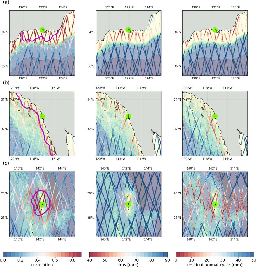
Ocean Sci., 17, 35–57, 2021 https://doi.org/10.5194/os-17-35-2021J. Oelsmann et al.: The zone of influence 41 use the Pearson correlation coefficient, the rmsSAT-TG and the We identify coherent zones of sea level variability rep- amplitude of the residual annual cycle between the TG and resented by different selection criteria in Fig. 1. The statis- SAT records. We compute each of those measures for every tics S are computed based on individual along-track SLA point of the 1 Hz along-track data (ALES) in combination time series (ALES) and GESLA TGs. We show different with the TG records from GESLA. As for ALES–GESLA- maps of these along-track statistics for (a) the Australian 250 km, TG data are interpolated onto the time step of the coast, (b) Californian coast and (c) Chichijima island (Japan). altimetry records. Correlations and rmsSAT-TG are computed The contour in the first column exemplifies the extent of a from the detrended TG and SAT time series. The amplitude ZOI, which represents a subset of 20 % of the best-correlated of the residual annual cycle is obtained from the remaining data. seasonal signal of the difference of the time series (SAT–TG). The obtained coherent structures reveal notable dependen- We acquire a dataset containing information on the perfor- cies on the local bathymetric and coastal properties. Fig- mance of multi-mission along-track data in the vicinity of ure 1a, for instance, shows far-reaching alongshore corre- every GESLA TG. The statistics are based on detrended data. lations, which is supported by all of the analyzed selec- Thus, all the metrics may be influenced by the similarity of tion criteria. In this example, the separation of the region the annual cycle. However, by repeating this analysis using of the coastal shelf–sea dynamics from the region of off- detrended and deseasoned data (not shown), no significant shore variability is in good agreement with the underlying differences are identified. bathymetric gradients. Kurapov et al. (2016) found similarly To define the ZOI, we select subsets of the data containing pronounced SLA coherency along the Californian coast, as the best-performing statistics (i.e., highest correlation, lowest shown in Fig. 1b. Based on model data and TG observa- rmsSAT-TG or residual annual cycle) above the Xth percentile tions, they explained the large-scale alongshore correlation according to the distribution of the statistic S in a 300 km pattern in part by the propagation of coastal trapped waves. radius around the TGs. Every subset (X, S) represents an in- In other locations such as Chichijima island (see Fig. 1c), dividual ZOI, in which we average SLAs in accordance with coastal and bathymetric control of SL is reduced and differ- the steps involved in the aforementioned 250 km radius selec- ent structures of coherency evolve. Consequently, the ZOI tion (ALES–GESLA-250 km; Sect. 3.1). The high-rate SLA can strongly vary in shape depending on the local coastal fea- time series (ALES) are then again subtracted from GESLA, tures and drivers of coastal variability. providing the ALES–GESLA–ZOI dataset for VLM estima- Comparing these three examples, we also observe that ab- tion (Sect. 3.3). solute values of the statistics differ from site to site. Corre- Note that in contrast to the 250 km selection, we ex- lations of along-track data near the Australian coastline, for tend the range in which SLAs are taken into account to instance, outperform the ones in the example in Fig. 1b. The 300 km to define the ZOI. The previous 250 km selection same holds for rmsSAT-TG values. These differences not only is, as in Kleinherenbrink et al. (2018), based on the space indicate different degrees of coherency, but can also stem autocorrelation scales of SLAs, which reflect characteris- from regional deviations in the quality of data, i.e., quality of tic eddy length scales (Stammer and Böning, 1992; Ducet TG records or error sources in the altimetric product, such as et al., 2000). These scales decrease towards higher latitudes tidal adjustments or coastal corrections. Differences can also (i.e., towards the poles) with changing internal Rossby ra- be caused by coastal properties, e.g., when the TGs are lo- dius. However, several studies found much larger correlation cated in sheltered areas, which separates the in situ variability length scales of SLAs, in particular along shorelines (Calafat from the one measured at distant altimeter tracks. We there- et al., 2018; Hughes and Meredith, 2006). Mechanisms other fore analyze the use of relative thresholds to select the SLAs, than mesoscale eddy activity were investigated to account since setting absolute thresholds as in Kleinherenbrink et al. for these coherent changes. One example is given by Calafat (2018) might not be applicable in all cases. Figure 1c also et al. (2018), who analyzed the driving factors of sea level shows that different statistics can determine different extents variability at the southeastern coast of the US. Using altime- of the ZOI, considering that rather poorly correlated areas try and three different ocean models, they found coherent are partially characterized by low residual annual cycle am- changes in the annual amplitude of SLAs over length scales plitudes. of thousands of kilometers along the coast from the Yucatán A correct choice of the ZOI based on a subset of high- Peninsula to Cape Hatteras. While the annual cycle signal performance SLAs can significantly reduce the SAT–TG itself was dominated by steric changes, with likewise large- residuals as exemplified in Fig. 2. Here, we show three time scale correlations at the continental slope, changes in the an- series of SAT–TG differences for the Australian site (see nual amplitude were argued to be dominated by boundary Fig. 1a). The first series (Fig. 2a) indicates much lower waves exerted by incident Rossby waves. Because we sim- residual noise when the time series is constructed from the ilarly find correlations beyond the 250 km length scale, in 20 % best SLAs (according to the rmsSAT-TG ). Here, the particular along elongated coastal regions (Fig. 1a and b), we ALES–GESLA–ZOI residuals outperform those of the other justify the larger 300 km radius. combinations (ALES–PSMSL-250 km and AVISO–PSMSL- https://doi.org/10.5194/os-17-35-2021 Ocean Sci., 17, 35–57, 2021
42                                                                                           J. Oelsmann et al.: The zone of influence

Figure 1. Zone of influence: different coherent zones of sea level variability are identified by different statistical criteria S. The columns
show correlations, rmsSAT-TG and the residual annual cycle from left to right. The metrics are computed on every point of the 1 Hz along-
track product, comparing the performance of altimetry measurements with the TGs, highlighted in green (center). (a) The southern coast
of Western Australia, (b) the western coast of North America (TG in San Diego) and (c) Chichijima island (Japan). The “color” contour in
the first column indicates a zone of influence built from 20 % of the best-correlated SLAs within a 300 km radius. The underlying contours
denote the underlying bathymetry.

250 km), which are still affected by a pronounced annual cy-             of the best-performing SLAs according to each criteria. For
cle not related to VLM.                                                  each threshold and criterion we derive an individual global
   While using relative thresholds can reduce the noise of               VLMSAT-TG trend and uncertainty dataset. We validate the
VLMSAT-TG time series for individual stations, we seek to                performance of the trend estimates for a specific ZOI defini-
identify a globally optimal ZOI definition and associated cri-           tion in accordance with Sect. 3.4. Optimal parameters X and
teria and thresholds, which lead to the largest improvements             S are then suggested for the global application (Sect. 4.2).
of uncertainty and accuracy of VLMSAT-TG . Therefore, we
vary the relative thresholds X between 0.0 and 0.975 (with
a step size of 0.025), which refers to using 100 % and 2.5 %

Ocean Sci., 17, 35–57, 2021                                                                      https://doi.org/10.5194/os-17-35-2021
J. Oelsmann et al.: The zone of influence                                                                                         43

                                                                      that are not common between the TG and altimeter obser-
                                                                      vation locations will also contribute to the SAT–TG differ-
                                                                      ences. Therefore, to avoid underestimation of the uncertainty
                                                                      of the parameters, we take into account autocorrelation in the
                                                                      residuals of the detrended and deseasoned time series. We
                                                                      describe the power spectral density of the noise with a com-
                                                                      bination of a power-law and a white noise model (using the
                                                                      Hector software; Bos et al., 2013). The power-law process
                                                                      assumes that time-correlated noise power is proportional to
                                                                      f κ , which for negative spectral indices κ describes increas-
                                                                      ing power at lower frequencies f and a white noise pro-
                                                                      cess when κ = 0 (Agnew, 1992). Santamaría-Gómez et al.
                                                                      (2011) showed that this combination (of a power-law and
                                                                      white noise model) represents the best approximation of the
                                                                      noise content for 275 GNSS station position time series.
                                                                      This combination was also implemented in studies concerned
                                                                      with VLMSAT-TG estimation (WM16; Kleinherenbrink et al.,
                                                                      2018; Ballu et al., 2019). In particular, the spectral index κ
                                                                      can contribute to detecting the intrusion of low-frequency
                                                                      signals in the differenced time series. Next to the spectral
                                                                      index κ we estimate the individual fractions of the power-
Figure 2. Shown are “SAT minus TG” time series for different
                                                                      law and white noise models, as well as the total variance σ 2 ,
datasets and configurations for the TG in Fig. 1a. (a) Monthly mean
                                                                      which scales the amplitude of the noise. We emphasize the
(mm) time series for ALES–GESLA when all SLAs are averaged in
a 300 km radius (blue) and when SLAs are comprised of the 20 %        fact that for individual regions other noise models could be
most representative anomalies based on the rmsSAT-TG between the      more appropriate than the implemented PL+WN model and
altimetry and TG (red). The grey line denotes the underlying high-    would thus yield more realistic uncertainty estimates. An ad-
frequency time series. (b) Monthly mean differenced time series for   vanced regional spectral analysis to identify the most suitable
ALES–PSMSL and AVISO–PSMSL, which are based on a 250 km               models is, however, beyond the scope of this study.
radius selection of SLAs. (c) Same as (b) but with the annual and
semi-annual signals removed.                                          3.4   Validation of VLMSAT-TG with VLMGNSS trends

                                                                      To validate SAT–TG-based trend estimates, we use the
3.3   Statistical analysis: trend and uncertainty                     ULR6a GPS solution provided by the GNSS data assem-
      estimation                                                      bly center SONEL (Systeme d’Observation du Niveau des
                                                                      Eaux Littorales, http://www.sonel.org, last access: 10 De-
We fit the differenced time series to a combination of a de-          cember 2020). The reanalysis covers 19 years of GNSS
terministic model and stochastic noise models with the max-           data from 1995 to 2014, which are processed within the
imum likelihood estimation (MLE) method. Parameters of                ITRF2008, consistent with the reference frame of altime-
the deterministic model are comprised of a constant offset A          try orbits. The primary coordinates provided by GNSS are
and a linear trend B. The annual and semi-annual signals are          geocentric Cartesian coordinates (X, Y, Z, Vx , Vy , Vz ). For
expressed by harmonic functions with the annual and semi-             the comparison with vertical trends inferred from other tech-
annual frequencies ω1,2 and amplitudes C1,2 and D1,2 .                niques, they are converted to ellipsoidal coordinates (lati-
                   2
                                                                      tude φ, longitude λ and ellipsoidal height h; Vφ , Vλ , Vh ).
                                                                      Thus, we compare GNSS ellipsoidal height trends (Vh ) with
                   X
y(t) = A + Bt +          Ci cos 2π tωi + Di sin 2π tωi         (1)
                   i=1
                                                                      SAT–TG trends. It should be mentioned that, while the al-
                                                                      timetry trends refer to the so-called TOPEX/Poseidon ellip-
   When combining altimetry and TGs for VLM estimation,               soid, the GNSS vertical trends refer to the GRS80 (Geodetic
several sources can contaminate the differenced time series           Reference System, 1980; Moritz, 2000) ellipsoid. Although
and inflate the actual “red” noise (low-frequency) content in         there is a difference of 70 cm between the semi-major axes
the residuals, which generates autocorrelated signals in the          of the two ellipsoids, the GNSS and SAT vertical trends can
data. The SLA computation is affected by the instrumental             be compared without degradation of precision, as both ellip-
errors of the range estimation and of each of the geophysi-           soids are geocentric and have the same orientation with re-
cal corrections (Ablain et al., 2009). Such errors, as well as        spect to the Earth’s body (e.g., the ellipsoid minor axes coin-
the measurement error of the TG itself, show up as residuals          cide with the Earth’s mean rotation axis, and the major axes
in the differenced time series. Moreover, sea level dynamics          are on the Earth’s equatorial plane). We take into account

https://doi.org/10.5194/os-17-35-2021                                                                  Ocean Sci., 17, 35–57, 2021
44 J. Oelsmann et al.: The zone of influence
Figure 3. (a) Global distribution of 52 common GESLA, PSMSL and ULR6 GNSS stations, which meet the described requirements.
(b) Number of TG stations sorted by the number of months which contain valid data (here shown in valid years) in the period 1993–2015.
GNSS stations which are closer than 1 km to a TG. With this with weights
constraint we aim to avoid potential differential vertical mo- r −1
tions between the TG and the GNSS antenna (WM16). 2 2
UGNSS + U SATTGi
The TG locations and record lengths differ among the pre- i
wi = !. (3)
sented experimental datasets (Sect. 3.1). Therefore, we de- Pn
r −1
2
UGNSS 2
+ USATTG
fine several requirements for the validation of those experi- i=1 i i
mental datasets to obtain a consistent set of TG and GNSS
validation pairs. In contrast to PSMSL records GESLA TG We also analyze the median of the absolute value of differ-
observations only last until 2015. Even when PSMSL TG ences (|1VLM|). This metric is less prone to extreme devi-
records are limited to before 2015, they still contain more ations and can thus consolidate the evaluation of the dataset
months of valid data than GESLA (see Fig. 3b). Hence, performances. We generally assume that GNSS provides a
we align the time period covered by the PSMSL TGs to more accurate estimation of the linear component of the
the corresponding GESLA TGs for all following experi- VLM with a smaller error than VLMSAT-TG , despite a shorter
mental datasets. Generally, we only take into account SAT– time span of measurements. Hence, for the purposes of this
TG time series when they cover at least 120 months of paper and as done in all studies concerning VLMSAT-TG esti-
valid data. Note that the outlier analysis (Sect. 2.4) or mation, we define as measures of accuracy the rms1VLM and
coupling of high-frequency TG data in the ZOI can re- additionally the median of |1VLM|. We include the spec-
duce the length of the SAT–TG time series for GESLA tral index κ (see Sect. 3.3) as it helps to understand the level
TGs. Taking into account all these requirements, we ob- of autocorrelation of the time series. All statistics other than
tain 52 common GESLA and PSMSL TGs that provide a the rms1VLM denote median values (of all VLMSAT-TG esti-
neighboring GNSS station within 1 km distance. These pairs mates) for a specific dataset configuration.
are validated for ALES–PSMSL-250 km, ALES–GESLA-
250 km and AVISO–PSMSL-250 km. The ALES–GESLA–
ZOI combination includes six more stations. The resulting 4 Results
validation pairs are shown in Fig. 3a, where a higher cover-
age in northerly and midlatitude regions is evident. 4.1 Comparison of different dataset configurations
We compute the rms1VLM and the median of the differ- based on a 250 km average selection
ences (1VLM) of VLMSAT-TG and VLMGNSS for a given
dataset combination. To take into account the derived formal We compare the performances of the three datasets which are
errors (U ) of the estimate we compute the weighted rmsw as constructed from 250 km radius SLA averages in Table 2.
follows: Validation against GNSS vertical velocities reveals that the
v gridded combination AVISO–PSMSL-250 km slightly out-
u n
uX performs ALES–PSMSL-250 km in terms of accuracy. Both
rmsw = t wi (VLMGNSSi − VLMSATTGi )2 , (2) the rms1VLM and the median of absolute trend differences
i=1 are 9 % lower for AVISO–PSMSL-250 km. This confirms
that, if all the available altimetry data within a wide region
are compared against monthly values of TGs, the use of a
gridded product outperforms the along-track performances
(WM16). Kleinherenbrink et al. (2018) similarly compared
Ocean Sci., 17, 35–57, 2021 https://doi.org/10.5194/os-17-35-2021J. Oelsmann et al.: The zone of influence 45
Table 2. Statistics of different SAT–TG combinations. 1VLM refers to the differences of VLMSAT-TG and VLMGNSS trends. X denotes the
relative level of comparability above which data are included.
X rms1VLM Weighted rms1VLM Med. |1VLM| Med. 1VLM Med. uncertainty Spectral index κ
mm yr−1 mm yr−1 mm yr−1 mm yr−1
ALES–PSMSL-250 km (52 stations)
1.68 1.57 1.28 −0.87 0.69 −0.39
AVISO–PSMSL-250 km (52 stations)
1.50 1.48 1.12 0.56 0.73 −0.56
ALES–GESLA-250 km (52 stations)
1.51 1.47 1.14 −0.39 0.79 −0.39
ALES–GESLA–ZOI (best rmsSAT-TG , 58 stations)
0 1.54 1.45 0.98 −0.46 0.86 −0.45
0.1 1.39 1.36 0.9 −0.27 0.86 −0.44
0.2 1.34 1.33 0.88 −0.36 0.83 −0.47
0.3 1.32 1.36 0.83 −0.44 0.78 −0.46
0.4 1.3 1.38 0.87 −0.37 0.76 −0.45
0.5 1.29 1.4 0.86 −0.26 0.73 −0.47
0.6 1.3 1.43 0.87 −0.31 0.71 −0.47
0.7 1.28 1.39 0.82 −0.41 0.66 −0.48
0.8 1.28 1.37 0.86 −0.41 0.58 −0.43
0.9 1.53 1.58 0.97 −0.43 0.61 −0.46
an along-track combination of 250 km SLA averages (from dex κ of the interpolated gridded product is lower than for
RADS) and PSMSL TG data with the AVISO–PSMSL com- the along-track data. Both κ indices (−0.56 and −0.39)
bination from WM16. They found a small rms1VLM reduc- also match those found by WM16 well for AVISO (−0.5)
tion of 0.1 mm yr−1 when using the along-track product with- and the along-track product (−0.4, GSFC). The larger spec-
out any correlation thresholds applied. WM16’s trends were, tral index (−0.39) is associated with reduced power of the
however, based on 1◦ radius averages of SLAs (in contrast to noise at low frequencies and thus indicates reduced con-
the 250 km selection), and record lengths were not equalized tamination of the SLA signal by sea level variations that
as in this study. do not represent those measured at the TG. This enhanced
For both combinations the median of the VLM differences comparability is also reflected in the lower trend uncer-
(ALES–PSMSL-250 km: −0.87 mm yr−1 ; AVISO–PSMSL- tainties of ALES–PSMSL-250 km (0.69 mm yr−1 ) compared
250 km: 0.56 mm yr−1 ) deviates from values shown in previ- to AVISO–PSMSL-250 km (0.73 mm yr−1 ). The differences
ous studies (WM16, −0.25 mm yr−1 ; Kleinherenbrink et al., between the characteristics of the residuals of the datasets
2018, −0.06 mm yr−1 ). In contrast to these previous esti- can partially be explained by the resolution of the data: due
mates, we use different spatial selection scales of SLAs, to the spatial filtering of the data, the gridded solution AVISO
smaller numbers of TG–GNSS pairs and deviating record incorporates information on SLAs beyond the 250 km radius
lengths, which impedes a direct comparison. Moreover, the and thus contains time-correlated SL signals with stronger
altimetry datasets might be affected by instrumental drifts. In deviations from the TG records.
this respect, differences among the datasets may be caused In comparison with the low-frequency datasets (ALES–
not only by different techniques applied to reduce inter- PSMSL-250 km and AVISO–PSMSL-250 km), the high-rate
mission biases (e.g., the MMXO approach for ALES), but setup ALES–GESLA-250 km improves the rms1VLM . The
also by different missions incorporated in the records. Note absolute bias of trend differences decreases more sub-
that in contrast to ALES, AVISO contains TOPEX, which stantially to 0.39 mm yr−1 (compared to −0.87 mm yr−1 ).
has also been shown to be affected by a strong drift (Wat- Compared to ALES–PSMSL-250 km, we find increased
son et al., 2015). Still, the observed rms1VLM of AVISO– trend uncertainties for ALES–GESLA-250 km, which can
PSMSL-250 km (1.50 mm yr−1 ) is comparable to the WM16 be partially explained by higher power-law variance of this
result (1.47 mm yr−1 ). In contrast to trend accuracies, the GESLA-based configuration. Although trend uncertainties
uncertainties are 5 % lower for ALES–PSMSL-250 km than are higher for the ALES–GESLA-250 km configuration, we
for AVISO–PSMSL-250 km. As in WM16, the spectral in- choose this setup to investigate the impact of the ZOI. This
https://doi.org/10.5194/os-17-35-2021 Ocean Sci., 17, 35–57, 202146 J. Oelsmann et al.: The zone of influence
Figure 4. Scatter and box plots comparing estimated SAT–TG trends and GNSS trends, as in WM16 Fig. 14. (a) ALES–PSMSL-250 km,
(b) AVISO–PSMSL-250 km, (c) ALES–GESLA-250 km and (d) ALES–GESLA–ZOI (at 20 % threshold based on the rms criterion). Error
bars denote the 1σ trend uncertainties of the individual estimates.
dataset provides better results concerning trend accuracy We observe that the rms1VLM , the median of absolute and
(weighted or unweighted rms) and has a lower median bias. total differences, and trend uncertainties decrease towards
Moreover, using the high-frequency data, we are able to cou- higher relative thresholds. The statistics converge to a min-
ple SAT and TG observations at much higher temporal res- imum when the ZOI is restricted to the 30 %–20 % best data.
olution than would be the case when using monthly PSMSL To compare ALES–GESLA–ZOI with the other dataset com-
data. Therefore, the ALES–GESLA coupling is further de- binations, we compute the statistics for the same 52 TGs
veloped based on a better definition of the ZOI in the next used in these configurations (because the shown statistic in
section. Table 2 refers to a larger set of 58 stations). At the 20 %
thresholds, we obtain similar performances with an rms1VLM
4.2 The zone of influence improves VLM estimates of 1.29 mm yr−1 , median uncertainty of 0.51 mm yr−1 and a
median of absolute differences (|1VLM|) of 0.86 mm yr−1 .
We investigate how the ZOI selection of SLAs fosters quality Thus, the improvements of rms1VLM compared to the plain
SAT–TG VLM estimates. As addressed in Sect. 3.2, we build 250 km radius selection (ALES–GESLA-250 km) are 15 %
the ZOI upon different criteria of comparability: rmsSAT-TG , and 35 % for uncertainties. Hence, we find more substantial,
correlation and the residual annual cycle. First, we focus on nearly linear reductions of trend uncertainty with increasing
the results of using the rmsSAT-TG of the detrended differ- relative thresholds compared to trend accuracy (rms1VLM ,
enced time series (Table 2 and Fig. 4, ALES–GESLA–ZOI).
Ocean Sci., 17, 35–57, 2021 https://doi.org/10.5194/os-17-35-2021You can also read