Role of jellyfish in the plankton ecosystem revealed using a global ocean biogeochemical model - Biogeosciences
←
→
Page content transcription
If your browser does not render page correctly, please read the page content below
Biogeosciences, 18, 1291–1320, 2021
https://doi.org/10.5194/bg-18-1291-2021
© Author(s) 2021. This work is distributed under
the Creative Commons Attribution 4.0 License.

Role of jellyfish in the plankton ecosystem revealed using a global
ocean biogeochemical model
Rebecca M. Wright1,2 , Corinne Le Quéré1 , Erik Buitenhuis1 , Sophie Pitois2 , and Mark J. Gibbons3
1 Tyndall Centre for Climate Change Research, School of Environmental Sciences,
University of East Anglia, Norwich, NR4 7TJ, UK
2 Centre for Environment, Fisheries and Aquaculture Science, Lowestoft, NR33 0HT, UK
3 Department of Biodiversity and Conservation Biology, University of the Western Cape,

Bellville 7535, Cape Town, Republic of South Africa

Correspondence: Rebecca M. Wright (rebecca.wright@uea.ac.uk)

Received: 17 April 2020 – Discussion started: 30 April 2020
Revised: 16 December 2020 – Accepted: 23 December 2020 – Published: 18 February 2021

Abstract. Jellyfish are increasingly recognised as important          1   Introduction
components of the marine ecosystem, yet their specific role is
poorly defined compared to that of other zooplankton groups.
This paper presents the first global ocean biogeochemical             Gelatinous zooplankton are increasingly recognised as influ-
model that includes an explicit representation of jellyfish and       ential organisms in the marine environment – not just for the
uses the model to gain insight into the influence of jelly-           disruptions they can cause to coastal economies (fisheries,
fish on the plankton community. The Plankton Type Ocean               aquaculture, beach closures, power plants, etc.; Purcell et al.,
Model (PlankTOM11) model groups organisms into plank-                 2007) – but also as important consumers of plankton (Lucas
ton functional types (PFTs). The jellyfish PFT is parame-             and Dawson, 2014), which is a food source for many ma-
terised here based on our synthesis of observations on jelly-         rine species (Lamb et al., 2017), and as key components in
fish growth, grazing, respiration and mortality rates as func-        marine biogeochemical cycles (Crum et al., 2014; Lebrato
tions of temperature and jellyfish biomass. The distribution          et al., 2012). The term gelatinous zooplankton can encom-
of jellyfish is unique compared to that of other PFTs in the          pass a wide range of organisms across three phyla: Tunicata
model. The jellyfish global biomass of 0.13 PgC is within             (salps), Ctenophora (comb jellies) and Cnidaria (true jelly-
the observational range and comparable to the biomass of              fish). This study focuses on Cnidaria (including Hydrozoa,
other zooplankton and phytoplankton PFTs. The introduction            Cubozoa and Scyphozoa), which contribute 92 % of the to-
of jellyfish in the model has a large direct influence on the         tal global biomass of gelatinous zooplankton (Lucas et al.,
crustacean macrozooplankton PFT and influences indirectly             2014). The other gelatinous zooplankton groups, Tunicata
the rest of the plankton ecosystem through trophic cascades.          and Ctenophora, are excluded from this study, because there
The zooplankton community in PlankTOM11 is highly sen-                are far fewer data available on their biomass and vital rates
sitive to the jellyfish mortality rate, with jellyfish increasingly   than for Cnidaria; they only contribute a combined global
dominating the zooplankton community as its mortality di-             biomass of 8 % of total gelatinous zooplankton (Lucas et
minishes. Overall, the results suggest that jellyfish play an         al., 2014). Cnidaria are both independent enough from other
important role in regulating global marine plankton ecosys-           gelatinous zooplankton and cohesive enough to be repre-
tems across plankton community structure, spatio-temporal             sented as a single plankton functional type (PFT) for global
dynamics and biomass, which is a role that has been gener-            modelling (Le Quéré et al., 2005). For the rest of this paper,
ally neglected so far.                                                pelagic Cnidaria are referred to as jellyfish.
                                                                         Jellyfish exhibit a radially symmetrical body plan and are
                                                                      characterised by a bell-shaped bodies (medusae). Swimming
                                                                      is achieved by muscular, “pulsing” contractions, and the an-

Published by Copernicus Publications on behalf of the European Geosciences Union.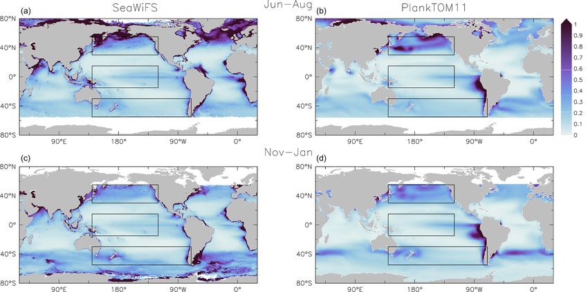
1292                                                           R. M. Wright et al.: Role of jellyfish in the plankton ecosystem

imals have one opening for both feeding and egestion. Most
scyphozoans and cubozoans, as well as many hydrozoans,
follow a meroplanktonic life cycle. A sessile (generally) ben-
thic polyp buds off planktonic ephyrae asexually. These, in
turn, grow into medusae that reproduce sexually to gen-
erate planula larvae, which then settle and transform into
polyps. Within this general life cycle, there is a large repro-
ductive and life-cycle variety, including some holoplanktonic
species that skip the benthic polyp stage, as well as holoben-
thic species that skip the pelagic phase, and much plasticity
(Boero et al., 2008; Lucas and Dawson, 2014).
   Jellyfish are significant consumers of plankton, feeding
mostly on zooplankton using tentacles and/or oral arms con-
taining stinging cells called nematocysts (Lucas and Daw-
son, 2014). The high body size to carbon content ratio of
jellyfish creates a large low-maintenance feeding structure,
which (because they do not use sight to capture prey) allow
them to efficiently clear plankton throughout 24 h (Acuña et
al., 2011; Lucas and Dawson, 2014). Jellyfish are connected
to lower trophic levels, with the ability to influence the plank-
ton ecosystem structure and thus the larger marine ecosystem
through trophic cascades (Pitt et al., 2007, 2009; West et al.,
2009). Jellyfish have the ability to rapidly form large high-
density aggregations known as blooms that can temporarily
dominate local ecosystems (Graham et al., 2001; Hamner and
Dawson, 2009). Jellyfish contribute to the biogeochemical           Figure 1. Schematic representation of the PlankTOM11 marine
cycle through two main routes: from life through feeding pro-       ecosystem model (see Table 1 for PFT definitions). (a) The plankton
                                                                    food web; arrows represent the grazing fluxes by protozooplankton
cesses, including the excretion of faecal pellets, mucus and
                                                                    (orange), mesozooplankton (red), macrozooplankton (blue) and jel-
messy-eating debris, and from death through the sinking of
                                                                    lyfish zooplankton (purple). Only fluxes with relative preferences
carcasses (Chelsky et al., 2015; Lebrato et al., 2012, 2013a;       above 0.1 are shown (see Table 3). (b) Source and sinks for dis-
Pitt et al., 2009). The high biomass achieved during jellyfish      solved organic carbon (DOC) and small (POCS ) and large (POCL )
blooms and the rapid sinking of excretions from feeding and         particulate organic carbon.
carcasses from such blooms make them a potentially signif-
icant vector for carbon export (Lebrato et al., 2013a, b; Luo
et al., 2020).                                                      ton, one bacteria and three zooplankton (Le Quéré et al.,
   Anthropogenic impacts from climate change, such as in-           2016). The three zooplankton groups are protozooplank-
creasing temperature and acidity (Rhein et al., 2013), and          ton (mainly heterotrophic flagellates and ciliates), mesozoo-
fishing, such as the removal of predators and competitors           plankton (mainly copepods) and macrozooplankton (as crus-
(Doney et al., 2012), impact the plankton including jellyfish       taceans, mainly euphausiids; see Table 1 for definitions). Jel-
(Boero et al., 2016; but see Richardson and Gibbons, 2008).         lyfish are therefore the fourth zooplankton group and 11th
Multiple co-occurring impacts make it difficult to understand       PFT in the PlankTOM model series. It introduces an addi-
the role of jellyfish in the marine ecosystem and how the role      tional trophic level to the ecosystem. To our knowledge, this
may be changed by the co-occurring impacts. The paucity of          is the first and only representation of jellyfish in a global
historical jellyfish biomass data, especially outside of coastal    ocean biogeochemical model at the time of writing. Plank-
regions and the Northern Hemisphere, has made it difficult          TOM11 is used to help quantify global jellyfish biomass and
to establish jellyfish global spatial distribution, biomass and     the role of jellyfish for the global plankton ecosystem.
trends from observations (Brotz et al., 2012; Condon et al.,
2012; Gibbons and Richardson, 2013; Lucas et al., 2014; Pitt
et al., 2018).                                                      2     Methods
   Models are useful tools to help understand the interactions
of multiple complex drivers in the environment. This paper          2.1    PLANKTOM11 model description
describes the addition of jellyfish to the Plankton Type Ocean
Model v. 10 (PlankTOM10; Le Quéré et al., 2016) global              PlankTOM11 was developed starting from the 10 PFT ver-
ocean biogeochemical model, which we call PlankTOM11.               sion of the PlankTOM model series (Le Quéré et al., 2016)
PlankTOM10 represents explicitly 10 PFTs: six phytoplank-           by introducing jellyfish as an additional trophic level at the

Biogeosciences, 18, 1291–1320, 2021                                                     https://doi.org/10.5194/bg-18-1291-2021
R. M. Wright et al.: Role of jellyfish in the plankton ecosystem                                                                        1293

Table 1. Size range and descriptions of PFT groups used in PlankTOM11. Adapted from Le Quéré et al. (2016).

 Name                    Abbre-      Size Range   Description and inclusions
                         viation            µm
 Autotrophs
 Picophytoplankton       PIC             0.5–2    Pico-eukaryotes and non-N2 -fixing cyanobacteria such as Synechococcus and Prochlorococcus
 N2 fixers               FIX             0.7–2    Trichodesmium and N2 -fixing unicellular cyanobacteria
 Coccolithophores        COC              5–10
 Mixed phytoplankton     MIX             2–200    e.g. autotrophic dinoflagellates and chrysophytes
 Diatoms                 DIA            20–200
 Phaeocystis             PHA           120–360    Colonial Phaeocystis
 Heterotrophs
 Bacteria                BAC              0.3–1   Here used to subsume both heterotrophic bacteria and archaea
 Protozooplankton        PRO             5–200    e.g. heterotrophic flagellates and ciliates
 Mesozooplankton         MES          200–2000    Predominantly copepods
 Macrozooplankton        MAC            > 2000    Euphausiids, amphipods and others, known as crustacean macrozooplankton
 Jellyfish zooplankton   JEL       200–> 20 000   Cnidaria medusae, “true jellyfish”

top of the plankton food web (Fig. 1a). A full description                huis et al., 2013b) and global surface chlorophyll from satel-
of PlankTOM10 is published in Le Quéré et al. (2016), in-                 lite observations (SeaWiFS, Sea-viewing Wide Field-of-view
cluding all equations and parameters. Here we provide an                  Sensor) are used to guide the model developments.
overview of the model development, focussing on the pa-                      The PlankTOM11 marine biogeochemistry component is
rameterisation of the growth and loss rates of jellyfish and              coupled online to the global ocean general circulation model
how these compare to the other macrozooplankton group. We                 Nucleus for European Modelling of the Ocean version 3.5
also describe the update of the relationship used to describe             (NEMO v3.5). We used the global configuration with a hor-
the growth rate as a function of temperature and subsequent               izontal resolution of 2◦ longitude by a mean resolution of
tuning. The formulation of the growth rate is the only equa-              1.1◦ latitude using a tripolar orthogonal grid. The vertical
tion that has changed since the previous version of the model             resolution is 10 m for the top 100 m, decreasing to a res-
(Le Quéré et al., 2016), although many parameters have been               olution of 500 m at 5 km depth, with a total of 30 vertical
modified (Sect. 2.1.6).                                                   z levels (Madec, 2013). The ocean is described as a fluid us-
   PlankTOM11 is a global ocean biogeochemistry model                     ing the Navier–Stokes equations and a nonlinear equation of
that simulates plankton ecosystem processes and their inter-              state (Madec, 2013). NEMO v3.5 explicitly calculates ver-
actions with the environment through the representation of                tical mixing at all depths using a turbulent kinetic energy
11 PFTs (Fig. 1). The 11 PFTs consist of six phytoplank-                  model and sub-grid eddy-induced mixing. The model is in-
ton (picophytoplankton, nitrogen-fixing cyanobacteria, coc-               teractively coupled to a thermodynamic sea-ice model (LIM
colithophores, mixed phytoplankton, diatoms and Phaeocys-                 version 2; Timmermann et al., 2005).
tis), bacteria and four zooplankton (Table 1). Physiological                 The temporal (t) evolution of zooplankton concentration
parameters are fixed within each PFT; therefore, within-PFT               (Zj ), including the jellyfish PFT, is described through the
diversity is not included. Spatial variability within PFTs is             formulation of growth and loss rates as follows:
represented through parameter dependence on environmen-
                                                                          ∂Zj   X Zj                      X4
tal conditions including temperature, nutrients, light and food               =  k
                                                                                   g F  × Fk × MGE × Zj −     gZk
                                                                                                           k=1 Zj
availability.                                                              ∂t         k

   The model contains 39 biogeochemical tracers, with full                                            Z
                                                                                   × Zk × Zj − R0◦j × dTZj × Zj                            (1)
marine cycles of key elements carbon, oxygen, phosphorus
and silicon, and simplified cycles of nitrogen and iron. There            (representing growth through grazing minus loss through
are three detrital pools: dissolved organic carbon (DOC),                 grazing minus basal respiration)
small particulate organic carbon (POCS ) and large particulate
organic carbon (POCL ). The elements enter through riverine                    Z                  Zj               X
                                                                          −m0◦j × cTZj ×        Zj
                                                                                                               ×    P
                                                                                                                   i i
fluxes and are cycled and generated through the PFTs via                                       K1/2 +     Zj
feeding, faecal matter, messy eating and carcases (Fig. 1b;
see Sect. 2.1.5 for detail; Buitenhuis et al., 2006, 2010,                (minus mortality).
2013a; Le Quéré et al., 2016). Model parameters are based                                                Z
                                                                            For growth through grazing, gFkj is the grazing rate by
on observations where available. A global database of PFT                 zooplankton Zj on food source Fk . This is a temperature-
carbon biomass that was designed for model studies (Buiten-               dependent Michaelis–Menten term that includes grazing

https://doi.org/10.5194/bg-18-1291-2021                                                               Biogeosciences, 18, 1291–1320, 2021
1294                                                             R. M. Wright et al.: Role of jellyfish in the plankton ecosystem

Table 2. Parameters used to calculate PFT-specific growth rate with
a three-parameter fit (Eq. 3) in PlankTOM11.

           PFT        µmax (d−1 )   Topt (◦ C)   dT (◦ C)
           FIX                0.2        27.6        8.2
           PIC                0.8        24.8       11.2
           COC                1.0        20.4        7.4
           MIX                1.1        34.0       20.0
           PHA                1.4        15.6       13.0
           DIA                1.3        23.2       17.2
           BAC                0.4        18.8       20.0
           PRO                0.4        22.0       20.0
           MES                0.4        31.6       20.0
           MAC                0.2        33.2       20.0
           JEL                0.2        23.6       18.8

preference (see Sect. 2.1.2). MGE is the modelled growth
efficiency (Buitenhuis et al., 2010). For loss through graz-
ing, gZ k
       Zj is the grazing of other zooplankton on Zj . For basal
                 Z
respiration, R0◦j is the respiration rate at 0 ◦ C, T is temper-
ature and dZj is the temperature dependence of respiration
(d10 = Q10 ). Mortality is the closure term of the model and is
mostly due to predation by higher trophic levels that are rep-
                            Z
resented by the model. m0◦j is the mortality rate at 0 ◦ C, cZj
is the temperature dependence of the mortality (c10 = Q10 )           Figure 2. Maximum growth rates for the 11 PFTs as a function of
       Zj                                                  P          temperature from observations (grey circles). The three-parameter
and K1/2  is the half saturation constant for mortality. i Pi         fit to data is shown in green, and the two-parameter fit is shown in
is the sum of all PFTs, excluding bacteria, and is used as a          blue, using the parameter values from Table 2. For full PFT names
proxy for the biomass of predators not explicitly included in         see Table 1. The R 2 values for both fits to data are given in Ap-
the model. More details on each term are provided below,              pendix Table A2.
and parameter values are given in Tables 2 to 5.

2.1.1   PFT growth                                                    function of temperature (µT ) is now defined by the optimal
                                                                      temperature (Topt ), maximum growth rate (µmax ) at Topt and
Growth rate is the trait that most distinguishes PFTs in mod-
                                                                      the temperature interval (dT ):
els (Buitenhuis et al., 2006, 2013a). Jellyfish growth rates
were compiled as a function of temperature from the litera-                                "               2 #
ture (see Appendix Table A1). In previous published versions                              − T − Topt
                                                                      µT = µmax     × exp                         .                   (3)
of the PlankTOM model, growth as a function of temperature                                    dT 2
(µT ) was fitted with two parameters:
                 T
                                                                      The available observations measure growth rate, but the
 T               10                                                   model requires specification of the grazing rate (Eq. 1).
µ = µ0 × Q10 ,                                                 (2)
                                                                      Growth of zooplankton and grazing (gT ) are related through
where µ0 is the growth at 0 ◦ C, Q10 is the temperature de-           the gross growth efficiency (GGE):
pendence of growth derived from observations and T is the
temperature (Le Quéré et al., 2016). Jellyfish growth rate is                 uT
poorly captured by an exponential fit to temperature. To bet-         gT =       .                                                    (4)
                                                                             GGE
ter capture the observations, the growth calculation has now
been updated with a three-parameter growth rate, which pro-           GGE is the portion of grazing that is converted to biomass.
duces a bell-shaped curve centred around an optimal growth            This was previously collated by Moriarty (2009) from the lit-
rate at a given temperature (Fig. 2 and Table 2). The three-          erature for crustacean and gelatinous macrozooplankton for
parameter fit is suitable for the global modelling of plankton,       the development of PlankTOM10. We extracted data for jel-
because it can represent an exponential increase if the data          lyfish from this collation (all scyphomedusae), which gave an
support this (Schoemann et al., 2005). The growth rate as a           average GGE of 0.29 ± 0.27 and n = 126 (Moriarty, 2009).

Biogeosciences, 18, 1291–1320, 2021                                                       https://doi.org/10.5194/bg-18-1291-2021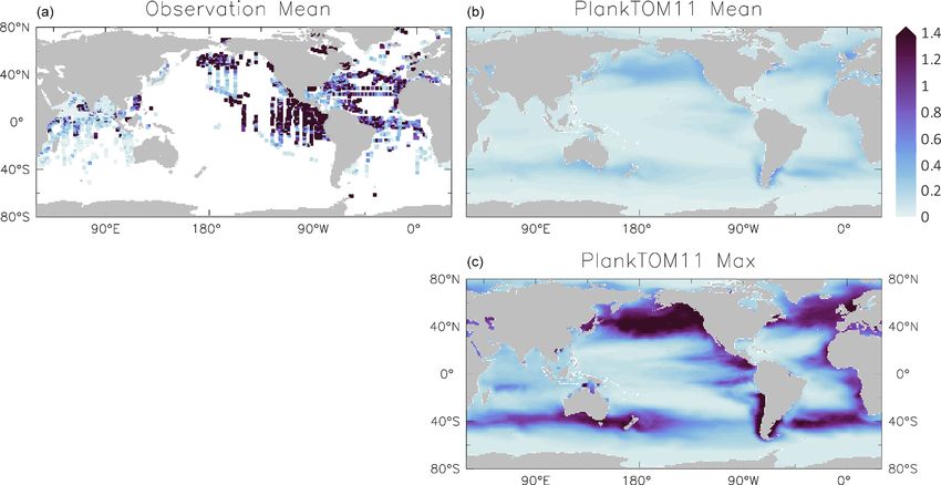
R. M. Wright et al.: Role of jellyfish in the plankton ecosystem                                                              1295

Table 3. Relative preference, expressed as a ratio, of zooplankton   relative preference of jellyfish for its prey assigned in the
for food (grazing) used in PlankTOM11. For each zooplankton, the     model, along with the preferences of the other zooplankton
preference ratio for diatoms is set to 1.                            PFTs. The zooplankton-relative preferences are based around
                                                                     a predator–prey size ratio, which by design is set to 1 for the
        PFT                       PRO    MES    MAC     JEL          zooplankton–diatom ratio. Preferences to other PFTs and to
        Autotrophs                                                   particulate carbon are then set relative to the preference for
                                                                     diatoms. The preference ratios are weighted using the global
        FIX                         2     0.1     0.1    0.1         carbon biomass for each type against a total food biomass
        PIC                         3    0.75     0.5    0.1
                                                                     weighted mean (sum of all the PFTs), calculated from the
        COC                         2    0.75       1    0.1
        MIX                         2    0.75       1      1
                                                                     MARine Ecosystem biomass DATa (MAREDAT) database,
        DIA                         1       1       1      1         following the methodology used for the other PFTs (Buiten-
        PHA                         2       1       1      1         huis et al., 2013a; Le Quéré et al., 2016). Zooplankton graz-
                                                                     ing is calculated using
        Heterotrophs
                                                                                         Z
        BAC                         4     0.1     0.1    0.1          Z        T
                                                                                     pFkj
        PRO                         0       2       1    7.5         gFkj   =µ  Zj    P Z     ,                                 (5)
        MES                         0       0       2     10                   K1/2 + pFkj Fk
        MAC                         0       0       0      5
                                                                               Z
        JEL                         0       0     0.5      0         where gFkj is the grazing rate by zooplankton Zj on food
        Particulate matter                                           source Fk as shown in Eq. (1), where µT is the growth rate
                                                                                              Z
        Small organic particles    0.1    0.1     0.1    0.1
                                                                     of zooplankton (Eq. 3), pFkj is the preference of the zooplank-
                                                                                                           Z
                                                                                                           j
        Large organic particles    0.1    0.1     0.1    0.1         ton for the food source (prey) and K1/2 is the half saturation
                                                                     constant of zooplankton grazing. The parameter values for
                                                                     grazing used in the model are given in Table 4.
2.1.2     Jellyfish PFT grazing                                      2.1.3    Jellyfish PFT respiration
The food web (and thus the trophic level of PFTs) is deter-          Previous analysis of respiration rates of jellyfish found that
mined through grazing preferences. The relative preference           temperature manipulation experiments with Q10 values of
of jellyfish zooplankton for the other PFTs was determined           > 3 were flawed, because the temperature was changed too
through a literature search (Colin et al., 2005; Costello and        rapidly (Purcell, 2009; Purcell et al., 2010). In a natural
Colin, 2002; Flynn and Gibbons, 2007; Malej et al., 2007;            environment, jellyfish gradually acclimate to temperature
Purcell, 1992, 1997, 2003; Stoecker et al., 1987; Uye and            changes, which has a smaller effect on their respiration rates.
Shimauchi, 2005a; see Appendix Table A3 for further detail).         Purcell et al. (2010) instead collated values from experiments
The dominant food source was mesozooplankton (specif-                that measured respiration at ambient temperatures, provid-
ically copepods), followed by protozooplankton (most of-             ing a range of temperature data across different studies. They
ten ciliates) and then macrozooplankton (Table 3). There is          found that Q10 for respiration was 1.67 for Aurelia species
little evidence for jellyfish actively consuming autotrophs.         (Purcell, 2009; Purcell et al., 2010). Moriarty (2009) col-
One of the few pieces of evidence is a gut content analy-            lated a respiration dataset for zooplankton, including gelati-
sis where “unidentified protists. . . some chlorophyll bearing”      nous zooplankton, using a similar selectivity as Purcell et
were found in a small medusa species (Colin et al., 2005).           al. (2010) for experimental temperature, feeding, time in cap-
Another is a study by Boero et al. (2007) which showed               tivity and activity levels. Jellyfish were extracted from the
that very small medusae such as Obelia will consume bac-             Moriarty (2009) dataset, which also included experiments on
teria and may consume phytoplankton. Studies on the diet             non-adult and non-Aurelia species medusae, unlike the Pur-
of the ephyrae life-cycle stage are limited in comparison to         cell et al. (2010) dataset. The relationship between tempera-
those on medusa, but the literature does show evidence for           ture and respiration is heavily skewed by body mass (Purcell
ephyrae consuming protists and phytoplankton (Båmstedt et            et al., 2010). The data were thus normalised by fitting to a
al., 2001; Morais et al., 2015). We assume that ephyrae are          general linear model (GLM) using a least squares cost func-
likely to have a higher preference for autotrophs, due to their      tion, to reduce the effect of body mass on respiration rates
smaller size as with the small medusa, but that this will have       (Ikeda, 1985; Le Quéré et al., 2016).
a minimal effect on the overall preferences and the biomass
consumed, so preferences for autotrophs are kept low. Once           GLM = log10 RR = a + b log10 BM + c T ,                    (6)
the relative preference is established, the absolute value of                                          !2
the preference is tuned to improve the biomass of the differ-                        X RT − RT
                                                                                          GLM      obs
                                                                     cost function =           T
                                                                                                          ,                     (7)
ent PFTs, as in Le Quéré et al. (2016). Table 3 shows the                                    Robs

https://doi.org/10.5194/bg-18-1291-2021                                                      Biogeosciences, 18, 1291–1320, 2021
1296                                                             R. M. Wright et al.: Role of jellyfish in the plankton ecosystem

Table 4. PlankTOM11 parameter values for macrozooplankton and jellyfish, with the associated equation.

                              Parameters                                    JEL          MAC      Equation
                              Respiration
                                Zj
                              R0◦ (d−1 )                                   0.03           0.01      Eq. (1)
                              dZj                                          1.88           2.46      Eq. (1)

                              Mortality
                                Zj
                              m0◦ (d−1 )                                    0.12           0.02     Eq. (1)
                              cZj                                           1.20           3.00     Eq. (1)
                              K Zj (µmol C L−1 )                    20.0 × 10⁻⁶    20.0 × 10⁻⁶      Eq. (1)
                              Growth and grazing
                              GGE                                           0.29           0.30     Eq. (4)
                              Grazing half saturation constant      10.0 × 10⁻⁶     9.0 × 10⁻⁶      Eq. (5)
                                Zj
                              K1/2 (µmol C L−1 )

                                                                                   Z
where RR is the respiration rate, BM is the body mass, and T             at 0 ◦ C (m0◦j in Eq. 1) of 0.018 per day. Sensitivity tests were
and R T are the observed temperature and associated respira-             carried out from this mortality rate due to low confidence in
tion rate respectively. The parameter values were then calcu-            the value.
lated using R0 = ea and Q10 = (ec )10 , where e is the expo-                Results from a subset of the sensitivity tests are shown
nential function. The resulting fit to data is shown in Fig. 3.          in Fig. 4. The model was found to best represent a range
The parameter values for respiration used in the model are               of observations when jellyfish mortality was increased to
given in Table 4. Macrozooplankton respiration values are                0.12 per day. The fit to data for mortality (µ0 = 0.018) and
also given in Fig. 3 and Table 4, to provide a comparison to             the adjusted mortality (µ0 = 0.12) is shown in Fig. 3. This
another zooplankton PFT of the most similar size available.              value was chosen based on expert judgement of the overall
                                                                         fit across multiple data streams. Although it was informed
2.1.4   Jellyfish PFT mortality                                          by the quantitative values in Table 6, the final choice re-
                                                                         quired the balance of positive and negative performance that
There are limited data on mortality rates for jellyfish, and             required expert judgement rather than a statistical number.
to use mortality data from the literature on any zooplank-               Mortality rate values closer to 0.018 per day allowed jelly-
ton group, some assumptions must be made (Acevedo et al.,                fish to dominate macro- and mesozooplankton, greatly re-
2013; Almeda et al., 2013; Malej and Malej, 1992; Mori-                  ducing their biomass (Figs. 4 and 5). Low jellyfish mortality
arty, 2009; Rosa et al., 2013). These assumptions are that the           also resulted in higher chlorophyll concentrations than ob-
population is in a steady state where mortality equals recruit-          served, especially in the high latitudes (Figs. 4 and 5; Bar-On
ment, reproduction is constant and mortality is independent              et al., 2018; Buitenhuis et al., 2013b). The adjusted mortal-
of age (Moriarty, 2009). All models with zooplankton mor-                ity rate used for PlankTOM11 may be accounting for sev-
tality rates follow these assumptions. In reality the mortality          eral components missing from experimental data, including
of a zooplankton population is highly variable. Steady states            the impact of higher-trophic-level grazing in the Avecedo
are balanced over a long period (if a population remains vi-             et al. (2013) study, which in copepods is 3–4 times higher
able), reproduction is restricted to certain times of year and           than other sources of mortality (Hirst and Kiørboe, 2002),
the early stages of life cycles are many times more vulner-              the greater vulnerability to mortality experienced during the
able to mortality. Despite these assumptions, with the lim-              early stages of the life cycle, and mortality due to parasites
ited data on mortality rates, the larger uncertainty lies with           and viruses, especially during blooms (Pitt et al., 2014).
the data rather than the assumptions (Moriarty, 2009). The                  PlankTOM11 uses a mortality rate for jellyfish that is
                                             Zj                          much higher than the limited observations (Figs. 4 and 5).
half saturation constant for mortality (K1/2     in Eq. 1) is set
                                                                         Lower jellyfish mortality is likely to be more representative
to 20 µmol C L−1 , which is the same as other zooplankton
                                                                         of adult life stages, as jellyfish experience high mortality dur-
types, due to the lack of PFT-specific data. In the small num-
                                                                         ing juvenile life stages, especially as planula larvae and dur-
ber of data available and suitable for use in the model (16 data
                                                                         ing settling (Lucas et al., 2012). The limited observations of
points from two studies), mortality ranged from 0.006–0.026
                                                                         jellyfish mortality are from mostly adult organisms, which
per day (Acevedo et al., 2013; Malej and Malej, 1992). Ap-
                                                                         may explain the dominance of jellyfish in the model when pa-
plying the exponential fit to these data gave a mortality rate

Biogeosciences, 18, 1291–1320, 2021                                                         https://doi.org/10.5194/bg-18-1291-2021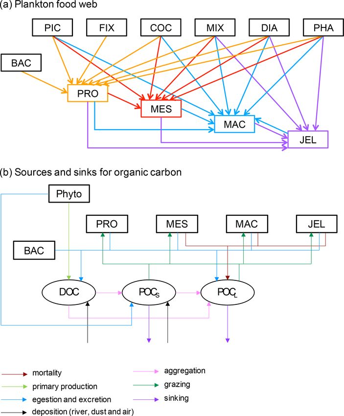
R. M. Wright et al.: Role of jellyfish in the plankton ecosystem                                                                                 1297

Figure 3. Maximum growth rates (a, b), respiration rates (c, d) and mortality rates (e, f) for jellyfish (left; purple) and macrozooplankton
(right; blue) PFTs as a function of temperature. The fit to data is shown in black, using the parameter values from Tables 2 and 4. Growth
rates are the same as shown in Fig. 2 but on a different scale. For jellyfish mortality, the thin dashed line is the fit to data, and the solid line is
the adjusted fit (Table 4).

rameterised with the observed mortality fit. The higher mor-                  zooplankton; it is generated from the mortality of mesozoo-
tality used for this study may be more representative of an                   plankton, macrozooplankton and jellyfish and is consumed
average across all life stages. Experimental jellyfish mortal-                through grazing by all zooplankton. The portion of POCS
ity is also likely to be lower than in situ mortality due to fac-             and POCL which is not grazed sinks through the water col-
tors such as senescence post-spawning and bloom conditions                    umn and is counted as export production at 100 m (Fig. 1b).
increasing the prevalence of disease and parasites and thus                   The sinking speed of POCS is 3 m d−1 , and the sinking speed
increasing mortality (Mills, 1993; Pitt et al., 2014). Using a                of POCL varies, depending on the concentration of ballast
higher mortality for this study is therefore deemed reason-                   and the resulting particle density. Proto-, meso- and macro-
able.                                                                         zooplankton excretion is largely in the form of particulate
                                                                              and solid faecal pellets, while this makes up very little of
2.1.5   Organic carbon cycling through the plankton                           jellyfish excretion. Jellyfish instead produce and slough off
        ecosystem                                                             mucus as part of their feeding mechanism (Pitt et al., 2009),
                                                                              which is represented in the model in the same way as the fae-
In PlankTOM11, the growth of phytoplankton modifies dis-                      cal pellet excretion, i.e. as a fraction of unassimilated grazing
solved inorganic carbon into DOC, which then aggregates                       contributing to POCL .
into POCS and POCL (Fig. 1b). POCS is also generated from
protozooplankton egestion and excretion and is consumed
through grazing by all zooplankton. POCL is also generated
by aggregation from POCS , egestion and excretion by all

https://doi.org/10.5194/bg-18-1291-2021                                                                  Biogeosciences, 18, 1291–1320, 2021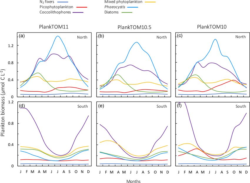
1298                                                              R. M. Wright et al.: Role of jellyfish in the plankton ecosystem

Figure 4. Results from sensitivity tests on jellyfish mortality rates. The adjusted fit simulation used for PlankTOM11 is shown by the black
filled circle, and the fit to the data simulation is shown by the grey filled circle; global mean PFT biomass (µmol C L−1 ) for 0–200 m depth
(a–e) and regional mean surface chlorophyll concentration (µg chl L−1 ; f–h) are shown. For the regional mean chlorophyll, the observations
are calculated from SeaWiFS. All data are averaged for 1985–2015, and between 30 and 55◦ latitude in both hemispheres: 140–240◦ E in the
north and 140–290◦ E in the south (see Fig. 8). “Phyto” is the sum of all the phytoplankton PFTs.

2.1.6   Additional tuning                                                   As shown in Eq. (1), there is a component in the mor-
                                                                         tality of zooplankton to represent predation by organisms
Following the change to the growth rate formulation (from                not included in the model. The jellyfish PFT is a significant
Eqs. 2 to 3), all PFT growth rates are lower compared to the             grazer of macrozooplankton and mesozooplankton (Table 3).
published version of PlankTOM10 (Le Quéré et al., 2016),                 To account for this additional grazing, the mortality term
but the change is largest for Phaeocystis, diatoms, bacteria             for macrozooplankton and the respiration term for mesozoo-
and protozooplankton (Fig. 2). Further tuning is carried out             plankton were reduced compared to model versions where
to rebalance the total biomass among phytoplankton PFTs                  no jellyfish are present (Table 5). Respiration is reduced in
following the change in formulation. The tuning included                 place of mortality for mesozooplankton as their mortality
increasing the grazing ratio preference of mesozooplankton               term had already been reduced to zero to account for pre-
for Phaeocystis and the grazing ratio preference of protozoo-            dation by macrozooplankton (Le Quéré et al., 2016). The
plankton for picophytoplankton within the limits of obser-               jellyfish PFT is also a significant grazer of protozooplank-
vations. Tuning also included increasing the half saturation             ton; however, following the adjustment of protozooplankton
constant of the phytoplankton Phaeocystis, picophytoplank-               grazing on picophytoplankton to account for changes to the
ton and diatoms for iron. The tuning resulted in a reduction             growth rate formulation and the low sensitivity of protozoo-
of Phaeocystis biomass and an increase in diatom biomass,                plankton to jellyfish mortality (Fig. 4), additional changes to
without disrupting the rest of the ecosystem. Diatom respira-            protozooplankton parameters were found to be unnecessary.
tion was also increased to reduce their biomass towards ob-
servations. Finally, bacterial biomass was increased closer to           2.1.7   Model simulations
observations by reducing the half saturation constant of bac-
teria for dissolved organic carbon and reducing the maximum              The PlankTOM11 simulations are run from 1920 to 2015,
bacteria uptake rate. See Appendix Table A4 for the parame-              forced by meteorological data including daily wind stress,
ter values before and after tuning.                                      cloud cover, precipitation and freshwater riverine input from

Biogeosciences, 18, 1291–1320, 2021                                                          https://doi.org/10.5194/bg-18-1291-2021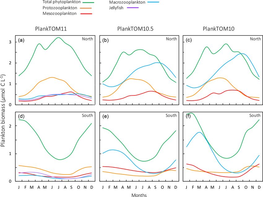
R. M. Wright et al.: Role of jellyfish in the plankton ecosystem                                                                        1299

Figure 5. Annual mean surface chlorophyll (µg chl L−1 ) and zooplankton carbon biomasses (µmol C L−1 ) of JEL, MAC, MES and PRO for
adjustment of JEL mortality for the simulation with a 0.02 mortality rate per day (left) and the adjusted fit simulation with a 0.12 mortality
rate per day (right) used in PlankTOM11. Results are shown for the surface box (0–10 m) and averaged for 1985–2015.

Table 5. Changes to non-jellyfish PFT parameters across the PlankTOM simulations. PlankTOM10LQ16 is the latest published version of
PlankTOM with 10 PFTs (Le Quéré et al., 2016), while PlankTOM10 is the simulation from this study.

                        Parameters          PlankTOM10LQ16         PlankTOM10       PlankTOM10.5       PlankTOM11
                        MAC mortality                    0.020             0.012              0.005            0.005
                        MES respiration                  0.014             0.014              0.001            0.001

NCEP/NCAR reanalysed fields (Kalnay et al., 1996). The                   ity of weather data (including by satellite) in 1980 compared
simulations start with a 28-year spin-up for 1920–1948                   to 1948, the dynamical fields are generally more represen-
where the meteorological conditions for year 1980 are used,              tative of small-scale structures than the earlier years. There
looping over a single year. Year 1980 is used as a typical aver-         is a small shock to the system at the start of meteorological
age year, as it has no strong El Niño/La Niña, as in Le Quéré            forcing, but this stabilises within a few years and decades be-
et al. (2010). Furthermore, because of the greater availabil-            fore the model output is used for analysis. Tests of different

https://doi.org/10.5194/bg-18-1291-2021                                                           Biogeosciences, 18, 1291–1320, 2021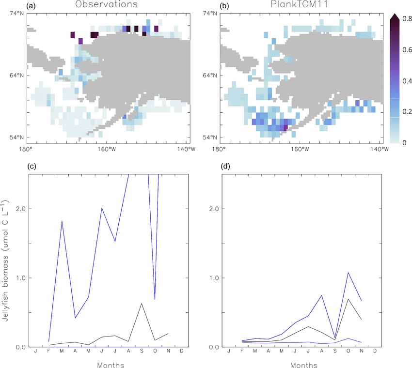
1300                                                          R. M. Wright et al.: Role of jellyfish in the plankton ecosystem

spin-up years were carried out in Le Quéré et al. (2010), in-      phylum down to species. The data cover the period from
cluding both 1948 and 1980, with little impact on trends gen-      August 1930 to August 2008 and contain abundance (indi-
erally. The spin-up is followed by interannually varying forc-     viduals m−3 , n = 107 156) and carbon biomass (µg C L−1 ,
ing for actual years from 1948–2015. All analysis is carried       n = 3406). The carbon biomass data are used over the abun-
out on the average of the last 31-year period of 1985–2015.        dance data despite the fewer data available, as they can be
PlankTOM11 is initialised with observations of dissolved in-       directly compared to PlankTOM11 results. Carbon biomass
organic carbon (DIC) and alkalinity (Key et al., 2004) after       is calculated from wet-weight to dry-weight conversion fac-
removing the anthropogenic component for DIC (Le Quéré             tors for species where data records are sufficient (Moriarty et
et al., 2010), NO3 , PO4 , SiO3 , O2 , temperature and salinity    al., 2013). The data were collected at depth ranging from 0
from the World Ocean Atlas (Antonov et al., 2010).                 to 2442 m. The majority of the data (97 %) was collected in
   Two further model simulations were carried out in order         the top 200 m with an average depth of 44 m (±32 m). Data
to better understand the effect of adding the jellyfish PFT.       from the top 200 m are included in the analysis. The original
The first simulation sets the jellyfish growth rate to 0, so       un-gridded biomass data were binned into 1◦ × 1◦ boxes at
it replicates the model set-up with 10 PFTs in Le Quéré            monthly resolution, as in Moriarty et al. (2013), reducing the
et al. (2016), which is here called PlankTOM10LQ16 , but it        number of gridded biomass data points to 849.
includes the updated growth formulation (Sect. 2.1.1) and             In MAREDAT, jellyfish biomass data are only present in
additional tuning (Sect. 2.1.5). The simulation is labelled        the Northern Hemisphere, which is likely to skew the data.
“PlankTOM10” in the figures. This simulation is otherwise          Another caveat against the data is that a substantially smaller
identical to PlankTOM11 except for the mortality term for          frequency of zeros is reported for biomass than for abun-
macrozooplankton and the respiration term for mesozoo-             dance. Under-reporting of zero values will increase the av-
plankton, which were initially returned to PlankTOM10LQ16          erage, regardless of the averaging method used. Biomass ob-
values, to account for the lack of predation by jellyfish.         servations from other global studies (Bar-On et al., 2018; Lu-
Macrozooplankton mortality was then tuned down from the            cas et al., 2014; Luo et al., 2020) are used conjunctly with the
PlankTOM10LQ16 value, from 0.02 to 0.012, to account for           global jellyfish biomass calculated here because of the poor
the change to the growth calculation (Table 5). The second         spatial coverage.
additional simulation is carried out to test the addition of an       To compare to the other PFTs within the MAREDAT
11th PFT in comparison to the addition of jellyfish as the         database, global jellyfish biomass was calculated according
11th PFT. This is done by parameterising the jellyfish PFT         to the methods in Buitenhuis et al. (2013b). Buitenhuis et
identically to the macrozooplankton PFT in PlankTOM11 so           al. (2013b) calculate a biomass range, using the median as
that there are 11 PFTs active, with two identical macrozoo-        the minimum and the arithmetic mean (AM) as the maxi-
plankton. This simulation is called PlankTOM10.5. The two          mum. The jellyfish zooplankton biomass range in MARE-
macrozooplankton in PlankTOM10.5 have mutual predation,            DAT was calculated as 0.46–3.11 PgC, with the median jel-
where they prey on each other, while the macrozooplank-            lyfish biomass almost as high as the microzooplankton and
ton in PlankTOM10 have no preference for themselves. Sub-          higher than meso- and macrozooplankton (Buitenhuis et al.,
sequently, macrozooplankton mortality in PlankTOM10.5 is           2013b). The jellyfish biomass range calculated here is used
kept the same as PlankTOM11 (Table 5) to account for the           to validate the new jellyfish component in the PlankTOM11
mutual predation. Otherwise, these simulations were identi-        model.
cal to PlankTOM11.

2.2    Jellyfish biomass observations                              3     Results

MARine Ecosystem biomass DATa (MAREDAT) is a                       3.1    Jellyfish biomass
database of global ocean plankton abundance and biomass,
which is harmonised to common units and is available online        The global jellyfish biomass estimated by various studies
as open-source data (Buitenhuis et al., 2013b). The MARE-          gives a range of results: 0.1 PgC (Bar-On et al., 2018), 0.32±
DAT database is designed to be used for the validation of          0.49 PgC (Lucas et al., 2014), 0.29 ± 0.56 PgC (Luo et al.,
global ocean biogeochemical models. MAREDAT contains               2020, updated from Lucas et al., 2014) and 0.46–3.11 PgC
global quantitative observations of jellyfish abundance and        calculated in this study (Sect. 2.2). Jellyfish biomass in
biomass as part of the generic macrozooplankton group (Mo-         PlankTOM11 is within the range but towards the lower end
riarty et al., 2013). The jellyfish subset of data has not been    of observations at 0.13 PgC, with jellyfish accounting for
analysed independently yet.                                        16 % of the total zooplankton biomass (Table 6). When the
   For this study, all MAREDAT records under the group             modelled biomass was tuned to match the higher observed
Cnidaria medusae (true jellyfish) were extracted from the          biomass by adjusting the mortality rate, jellyfish dominate
macrozooplankton group (Moriarty et al., 2013) and exam-           the entire ecosystem significantly, reducing levels of the
ined. The taxonomic level within the database varies from          other zooplankton and increasing chlorophyll above observa-

Biogeosciences, 18, 1291–1320, 2021                                                   https://doi.org/10.5194/bg-18-1291-2021
R. M. Wright et al.: Role of jellyfish in the plankton ecosystem                                                                             1301

Figure 6. Jellyfish carbon biomass (µmol C L−1 ) in PlankTOM11 and in observations from the Jellyfish Database Initiative (Luo et al.,
2020). PlankTOM11 results (b, c) are the mean and maximum biomass from monthly climatologies. Observations (a) are the mean biomass;
areas with no observations are in white. Observations are on a 1◦ × 1◦ grid and are plotted using a three-cell averaging filler for visual clarity.
All data are for 0–200 m. The gridded observation data are only available as a mean over time and depth (Luo et al., 2020). Due to the patchy
nature of the observations in depth and time, the mean may be skewed high or low, while the model is sampled across the full time and depth.

tions for the Northern Hemisphere and Southern Hemisphere                   the range of observations in the top 200 m (Fig. 6). Plank-
(Figs. 4 and 5).                                                            TOM11 overestimates the minimum values and underesti-
   PlankTOM11 generally replicates the patterns of jellyfish                mates the maximum values. However, part of this discrep-
biomass with observations. High biomass occurs at around                    ancy may be due to under-sampling in the observations. A
50–60◦ N across the oceans, with the highest biomass in the                 key caveat in jellyfish data is that the data are not uniformly
North Pacific. PlankTOM11 also replicates low biomass in                    distributed spatially or temporally and not proportionally dis-
the Indian Ocean, and the eastern half of the tropical Pacific              tributed between various biomes of the ocean, with collection
shows higher biomass compared to other open ocean areas                     efforts skewed to coastal regions and the Northern Hemi-
in agreement with patterns in observations (Fig. 6; Lucas et                sphere (MAREDAT; Lilley et al., 2011; Lucas et al., 2014;
al., 2014; Luo et al., 2020). However, PlankTOM11 under-                    Luo et al., 2020). This sampling bias and the sampling meth-
estimates the high jellyfish biomass in the tropical Pacific                ods also tend to favour larger, less delicate species, which are
(Fig. 6). Most of the data informing the jellyfish parameters               often scyphomedusae with a meroplanktonic life cycle.
are from temperate species, so the model will better represent                 Jellyfish are characterised by their bloom and bust dy-
higher latitudes compared to lower latitudes. This is likely re-            namic, resulting in patchy and ephemeral biomass. The mean
sponsible for some of the underestimation of biomass in this                to max biomass ratio of observations (MAREDAT) was com-
region. The competition of jellyfish with macrozooplankton                  pared to the same ratio for PlankTOM11 to assess the replica-
also plays a role (see Sect. 3.3 for further discussion). The               tion of this characteristic. The observations give a wide range
lack of biomass observations around 40◦ S makes it difficult                of ratios depending on the type of mean used. The Plank-
to determine if the peak in jellyfish biomass in PlankTOM11                 TOM11 ratio falls within this range but towards the lower
at this latitude is representative of reality. The maximum                  end (Table 7). PlankTOM11 replicates some of the patchy
biomass in the Southern Hemisphere is mostly around coastal                 and ephemeral biomass of jellyfish.
areas, i.e. South America and southern Australia (Fig. 6).                     Jellyfish biomass in MAREDAT has poor global spatial
This is expected from reports and papers on jellyfish in these              coverage. The region around the coast of Alaska has the
areas (Condon et al., 2013; Purcell et al., 2007, and refer-                highest density of observations and is used here to evalu-
ences therein). A prevalence of jellyfish in coastal areas is ap-           ate the mean, range and seasonality of the carbon biomass
parent (Fig. 6), in line with observations (Lucas et al., 2014;             of jellyfish as represented in PlankTOM11. The gridded jel-
Luo et al., 2020), even without any specific coastal advan-                 lyfish observations from Luo et al. (2020; see Fig. 6) are
tages for jellyfish in the model (see macrozooplankton in Le                available as a mean over time and depth, so they cannot be
Quéré et al., 2016). However, PlankTOM11 underestimates                     used to evaluate range or seasonality. Spatially, the observa-

https://doi.org/10.5194/bg-18-1291-2021                                                               Biogeosciences, 18, 1291–1320, 2021
1302 R. M. Wright et al.: Role of jellyfish in the plankton ecosystem
Table 6. Global mean values for rates and biomass from observations and the PlankTOM11 and PlankTOM10 models averaged over 1985–
2015. In parenthesis is the percentage share of the plankton type of the total phytoplankton or zooplankton biomass. The percentage share
of mixed phytoplankton is not included, as there are no mixed-phytoplankton observations; therefore, the phytoplankton percentages are of
total phytoplankton minus mixed phytoplankton. References for observations are given in Appendix Table A5.
PlankTOM11 PlankTOM10 Observations
Rates
Primary production (PgC yr−1 ) 41.6 43.4 51–65
Export production at 100 m (PgC yr−1 ) 7.1 7.0 5–13
CaCO3 export at 100 m (PgC yr−1 ) 1.3 1.2 0.6–1.1
N2 fixation (TgN yr−1 ) 97.2 95.9 60–200
Phytoplankton biomass 0–200 m (PgC)
N2 fixers 0.065 (8 %) 0.075 (10 %) 0.008–0.12 (2 %–8 %)
Picophytoplankton 0.141 (17 %) 0.153 (20 %) 0.28–0.52 (35 %–68 %)
Coccolithophores 0.248 (30 %) 0.212 (27 %) 0.001–0.032 (0.2 %–2 %)
Mixed phytoplankton 0.263 0.268 –
Phaeocystis 0.177 (22 %) 0.170 (22 %) 0.11–0.69 (27 %–46 %)
Diatoms 0.183 (22 %) 0.167 (21 %) 0.013–0.75 (3 %–50 %)
Total phytoplankton biomass 1.077 1.046 0.412–2.112
Heterotrophs biomass 0–200 m (PgC)
Bacteria 0.041 0.046 0.25–0.26
Protozooplankton 0.295 (36 %) 0.330 (32.7 %) 0.10–0.37 (27 %–31 %)
Mesozooplankton 0.193 (23 %) 0.218 (21.6 %) 0.21–0.34 (25 %–66 %)
Macrozooplankton 0.205 (25 %) 0.460 (45.6 %) 0.01–0.64 (3 %–47 %)
Jellyfish zooplankton 0.129 (16 %) – 0.10–3.11
Total zooplankton biomass 0.823 1.008 0.42–4.46
Table 7. Jellyfish biomass globally from observations (MAREDAT) over the summer followed by a large peak in September in the
and PlankTOM11. Three types of mean are given for the observa- observations and in October in PlankTOM11 (Fig. 7). Over-
tions; Med is the median, AM is the arithmetic mean and GM is the all, PlankTOM11 replicates the mean but underestimates the
geometric mean. The ratios are all scaled to mean = 1. All units are maximum biomass and temporal patchiness of the observa-
in µg C L−1 . tions (Fig. 7 and Table 8).
Mean Max Ratio
3.2 Ecosystem properties of PLANKTOM11
Observations AM 3.61 156.0 1 : 43
GM 0.95 156.0 1 : 165
PlankTOM11 reproduces the main characteristics of surface
Med 0.29 156.0 1 : 538
chlorophyll observations, with high chlorophyll concentra-
PlankTOM11 AM 1.18 98.9 1 : 84 tion in the high latitudes, low concentration in the subtrop-
ics and elevated concentrations around the Equator (Fig. 8).
PlankTOM11 also reproduces higher chlorophyll concentra-
tions in the northern Pacific compared to the southern Pacific
tions peak around the north coast of Alaska, while Plank- (Fig. 9) and higher concentrations in the southern Atlantic
TOM11 peaks around the south coast (Fig. 7). This differ- compared to the southern Pacific Ocean (Fig. 8). Overall the
ence is likely due to the lack of small-scale physical pro- model underestimates chlorophyll concentrations, as is stan-
cesses in the model due to the relatively coarse model res- dard with models of this type (Le Quéré et al., 2016), par-
olution. PlankTOM11 reproduces the observed mean jelly- ticularly in the central and northern Atlantic. PlankTOM11
fish biomass around the coast of Alaska (0.16 compared to also captures the seasonality of chlorophyll, with concentra-
0.13 µmol C L−1 ), but it underestimates the maximum and tions increasing in summer compared to the winter for each
spread of the observations (Table 8). The spatial patchiness hemisphere (Fig. 8).
is somewhat replicated in PlankTOM11, although with a To assess the effect of adding jellyfish to PlankTOM, two
smaller variation (Fig. 7). PlankTOM11 replicates the mean additional simulations were conducted: PlankTOM10 where
seasonal shape and biomass of jellyfish with a small peak jellyfish growth is set to zero and PlankTOM10.5 where all
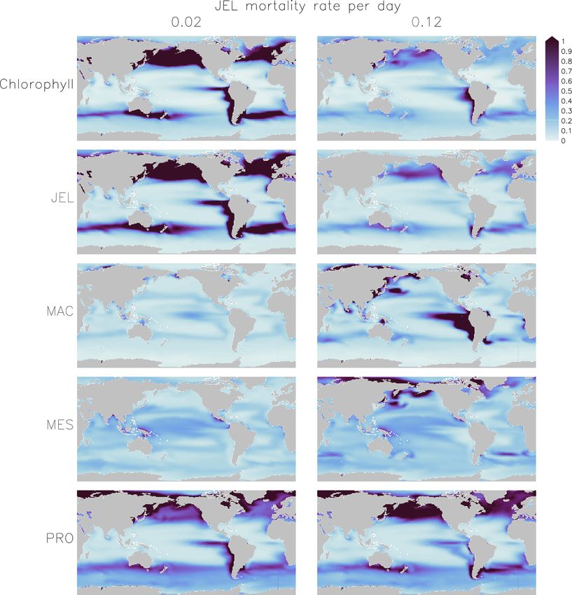
Biogeosciences, 18, 1291–1320, 2021 https://doi.org/10.5194/bg-18-1291-2021R. M. Wright et al.: Role of jellyfish in the plankton ecosystem 1303 Figure 7. Carbon biomass of jellyfish (µmol C L−1 ) from MAREDAT observations (a, c) and PlankTOM11 (b, d) for the coast of Alaska (the region with the highest density of observations). Panels (a, b) show the mean jellyfish biomass, and panels (c, d) the seasonal jellyfish biomass, with the monthly mean in black and the monthly minimum and maximum in blue. Observations and PlankTOM11 results are for 0–150 m, as the depth range where > 90 % of the observations occur. No observations were available for January or December. Figure 8. Surface chlorophyll (µg chl L−1 ) averaged for June to August (a, b) and November to January (c, d). Panels show observations from the SeaWiFS (a, c) satellite and results from PlankTOM11 (b, d). Observations and model are averaged for 1997–2006. The black boxes show the Pacific northern, tropical and southern regions used in Figs. 4 and 9. https://doi.org/10.5194/bg-18-1291-2021 Biogeosciences, 18, 1291–1320, 2021
1304                                                              R. M. Wright et al.: Role of jellyfish in the plankton ecosystem

Figure 9. Surface chlorophyll for observations from the SeaWiFS satellite, PlankTOM11, PlankTOM10.5 and PlankTOM10. Regional
chlorophyll concentration is in µg chl L−1 (a) for the northern (N), tropical (T) and southern (S) Pacific Ocean regions shown in Fig. 8 and
the N/S chlorophyll concentration ratio (b). Observations and model are averaged for 1997–2006.

jellyfish parameters are set equal to macrozooplankton pa-              from observations (Table 6). PlankTOM11 is dominated by
rameters (Sect. 2.1.6). The two simulations show similar                mixed phytoplankton and coccolithophores, together making
spatial patterns of surface chlorophyll to PlankTOM11 but               up 47 % of the total phytoplankton biomass. Diatoms and
different concentration levels. PlankTOM11 closely repli-               Phaeocystis are the next most abundant and fall within the
cates the chlorophyll ratio between the north and south Pa-             observed range, followed by picophytoplankton with around
cific with a ratio of 2.12 compared to the observed ratio of            half the observed biomass (Table 6). The observations are
2.16 (Fig. 9). PlankTOM10 and PlankTOM10.5 underesti-                   dominated by picophytoplankton, followed by Phaeocystis
mate the observed ratio with ratios of 1.57 and 1.96 respec-            and diatoms (Table 6). The modelled mixed phytoplankton
tively (Fig. 9). Adding an 11th PFT improves the chloro-                is likely taking up the ecosystem niche of picophytoplank-
phyll ratio; however, the regional chlorophyll concentrations           ton. Coccolithophores are overestimated by a factor of 10 and
for PlankTOM10.5 are a poorer match to the observations                 may also be filling the ecosystem niche of picophytoplankton
than PlankTOM11, especially in the north (Fig. 9). Plank-               in the model (Table 6). The phytoplankton community com-
TOM10 overestimates the observed chlorophyll concentra-                 position changed from PlankTOM10LQ16 to PlankTOM11,
tion in the south (0.22 and 0.18 respectively; Fig. 9). All             with some phytoplankton types moving closer to observa-
three simulations underestimate chlorophyll concentration in            tions and some moving further away. For example, for N2 fix-
the tropics compared to observations (Fig. 9). The north-to-            ers PlankTOM11 is in line with the upper end of observations
south chlorophyll ratio metric was developed by Le Quéré et             at 8 %, while PlankTOM10 and PlankTOM10LQ16 overesti-
al. (2016) as a simple method to quantify model performance             mate N2 fixers (10 % and 11 % respectively). For picophyto-
for emergent properties, focussing on the Pacific Ocean as              plankton, PlankTOM10LQ16 is within the range of observa-
the area where this ratio is most pronounced in the observa-            tions at 38 %, while PlankTOM11 and PlankTOM10 under-
tions. These simulations further support the suggestion by Le           estimate the community share of picophytoplankton (17 %
Quéré et al. (2016) that the observed distribution of chloro-           and 20 % respectively). For Phaeocystis, all three simula-
phyll in the north and south is a consequence of trophic bal-           tions underestimate the community share, but PlankTOM11
ances between the PFTs and improves with increasing plank-              and PlankTOM10 (both 22 %) are closer to the lower end
ton complexity.                                                         of observations (27 %) than PlankTOM10LQ16 (15 %; Table
   PlankTOM11 underestimates primary production by                      6; Le Quéré et al., 2016). Overall, the difference between
10 PgC yr−1 , which is similar to the underestimation in                PlankTOM10LQ16 and PlankTOM11 is greater than the dif-
PlankTOM10LQ16 of 9 PgC yr−1 . As suggested by Le Quéré                 ference between PlankTOM10 and PlankTOM11, suggesting
et al. (2016), this may be due to the model only represent-             that the change to growth of PFTs had a larger effect on phy-
ing highly active bacteria, which is unchanged between the              toplankton community composition than the addition of jel-
model versions, while observed biomass is also from low-                lyfish. This is expected, as the growth change directly effects
activity bacteria and ghost cells. Export production and N2             each PFT and model results are sensitive to PFT growth rates
fixation are within the observational range, and CaCO3 ex-              (Buitenhuis et al., 2006, 2010). Jellyfish affect phytoplankton
port is slightly overestimated (Table 6).                               community composition, but the effect is small.
   In PlankTOM11 each PFT shows a unique spatial distri-
bution in carbon biomass (Fig. 5). The total biomass of phy-
toplankton is within the range of observations, but the parti-
tioning of this biomass between phytoplankton types differs

Biogeosciences, 18, 1291–1320, 2021                                                         https://doi.org/10.5194/bg-18-1291-2021
R. M. Wright et al.: Role of jellyfish in the plankton ecosystem                                                                     1305

Figure 10. Zonal mean distribution for the PlankTOM11, PlankTOM10.5 and PlankTOM10 simulations. All plankton biomass data are for
the surface box (0–10 m). For PlankTOM10.5, the MAC PFT has been summed with the 11th PFT that duplicates MAC. The bottom panels
are the zonal mean distribution of primary production, integrated over the top 100 m, and export production at 100 m. All data are averaged
for 1985–2015.

3.3   Role of jellyfish in the plankton ecosystem                       teract to affect the rate of consumption (Eq. 5). The great-
                                                                        est difference in PFT biomass, especially macrozooplankton
Macrozooplankton exhibit the largest change in biomass be-              biomass, between simulations occurs in latitudes higher than
tween the three simulations, followed by mesozooplankton                30◦ where jellyfish biomass is highest (Fig. 10). In the trop-
(Fig. 10). This is despite the higher preference of jellyfish           ics, jellyfish have a low impact on the ecosystem due to their
grazing on mesozooplankton (ratio of 10) than on macro-                 low biomass in this region (Figs. 6 and 10).
zooplankton (ratio of 5; Table 3). The central competition                 The seasonality of the PFTs in each simulation is shown
for resources between jellyfish and macrozooplankton is that            in Fig. 11 for 30–70◦ north and south, as the regions with the
they both preferentially graze on mesozooplankton, then on              greatest differences between simulations (Fig. 10). In Plank-
protozooplankton, although macrozooplankton have a lower                TOM10, macrozooplankton represent the highest trophic
preference ratio for zooplankton than jellyfish, as more of             level. The addition of another PFT at the same or at a
their diet is made up by phytoplankton (Table 3). In sim-               higher trophic level (PlankTOM10.5 and PlankTOM11 re-
ple terms, this means that for two equally sized popula-                spectively) reduces the biomass of the macrozooplankton
tions of jellyfish and macrozooplankton, jellyfish would con-           through a combination of competition and low-level preda-
sume more meso- and protozooplankton than would be con-                 tion (Figs. 10 and 11). For PlankTOM10.5 results, macrozoo-
sumed by macrozooplankton. However, predator biomass,                   plankton is summed with the 11th PFT (identical to macro-
prey biomass and the temperature dependence of grazing in-

https://doi.org/10.5194/bg-18-1291-2021                                                         Biogeosciences, 18, 1291–1320, 2021
1306 R. M. Wright et al.: Role of jellyfish in the plankton ecosystem Figure 11. Seasonal surface carbon biomass (µmol C L−1 ) of total phytoplankton PFTs, protozooplankton, mesozooplankton, macrozoo- plankton and jellyfish. For PlankTOM10.5, the MAC PFT has been summed with the 11th PFT that duplicates MAC. Panels shown PFT biomass for PlankTOM11 (a, d), PlankTOM10.5 (b, e) and PlankTOM10 (c, f) for two regions; the north, 30–70◦ N (a–c), and the south 30–70◦ S (d–f), across all longitudes. All data are averaged for 1985–2015. zooplankton in this simulation). The addition of this 11th protozooplankton whilst jellyfish simultaneously provide an PFT at the same trophic level reduces the biomass of the additional predation pressure on meso- and protozooplank- macrozooplankton (Figs. 10 and 11), despite the macro- ton. The decrease in predation by macrozooplankton may be zooplankton mortality being reduced from PlankTOM10 to compensated for by the increase in predation by jellyfish, re- PlankTOM10.5 (Table 5), which would be expected to in- sulting in only a small change to the overall biomass of meso- crease macrozooplankton biomass. However, the low level of zooplankton and protozooplankton. mutual predation between the two macrozooplankton PFTs In PlankTOM11, there is a clear distinction between the slightly reduces their overall biomass. This reduction in biomass in the north and south, with higher biomass for each biomass mostly occurs during the autumn macrozooplank- PFT in the north compared to the south (Figs. 10 and 11). ton bloom, where the peak is reduced from PlankTOM10 Plankton types have higher concentrations in the respective to PlankTOM10.5, while the winter to spring biomass is hemisphere’s summer and a double peak in phytoplankton in similar across the two simulations (Fig. 11). The drop in the north (Fig. 11). PlankTOM10 also has a higher biomass mesozooplankton respiration from PlankTOM10 to Plank- of each PFT in the north compared to the south, but the differ- TOM10.5 (Table 5) lowers the rate of respiration, especially ence is smaller than that in PlankTOM11 (Figs. 10 and 11). at lower temperatures. This likely accounts for the increase in The key difference between the two models is the biomass PlankTOM10.5 mesozooplankton biomass at higher latitudes of macrozooplankton. In PlankTOM10, macrozooplankton (Fig. 10). The addition of jellyfish changes the zooplankton are the dominant zooplankton, especially in late summer and with the highest biomass from macrozooplankton to proto- autumn where their biomass matches and even exceeds the zooplankton and reduces the biomass of mesozooplankton, biomass of phytoplankton in the region (Fig. 11). In Plank- in both the north and south (Fig. 11). However, the impact TOM11, neither macrozooplankton nor any other zooplank- on the biomass of mesozooplankton and protozooplankton is ton come close to matching the biomass of phytoplankton. small, despite mesozooplankton being the preferential prey The largest direct influence of jellyfish in these regions is of jellyfish, followed by protozooplankton. The small im- its role in controlling macrozooplankton biomass through pact of jellyfish on mesozooplankton and protozooplankton competition for prey resources, particularly mesozooplank- biomass may be due to trophic cascade effects where jelly- ton and protozooplankton, and through the predation of jel- fish reduce the biomass of macrozooplankton, which reduces lyfish on macrozooplankton. the predation pressure of macrozooplankton on meso- and Biogeosciences, 18, 1291–1320, 2021 https://doi.org/10.5194/bg-18-1291-2021
You can also read