An improved air mass factor calculation for nitrogen dioxide measurements from the Global Ozone Monitoring Experiment-2 (GOME-2) - Atmos. Meas. Tech
←
→
Page content transcription
If your browser does not render page correctly, please read the page content below
Atmos. Meas. Tech., 13, 755–787, 2020
https://doi.org/10.5194/amt-13-755-2020
© Author(s) 2020. This work is distributed under
the Creative Commons Attribution 4.0 License.

An improved air mass factor calculation for nitrogen dioxide
measurements from the Global Ozone Monitoring
Experiment-2 (GOME-2)
Song Liu1 , Pieter Valks1 , Gaia Pinardi2 , Jian Xu1 , Athina Argyrouli4,1 , Ronny Lutz1 , L. Gijsbert Tilstra3 ,
Vincent Huijnen3 , François Hendrick2 , and Michel Van Roozendael2
1 Deutsches Zentrum für Luft- und Raumfahrt (DLR), Institut für Methodik der Fernerkundung (IMF),
Oberpfaffenhofen, Germany
2 Royal Belgian Institute for Space Aeronomy (BIRA-IASB), Brussels, Belgium
3 Royal Netherlands Meteorological Institute (KNMI), De Bilt, the Netherlands
4 Technical University of Munich (TUM), Department of Civil, Geo and Environmental Engineering,

Chair of Remote Sensing Technology, Munich, Germany

Correspondence: Song Liu (song.liu@dlr.de)

Received: 10 July 2019 – Discussion started: 14 August 2019
Revised: 14 December 2019 – Accepted: 21 January 2020 – Published: 18 February 2020

Abstract. An improved tropospheric nitrogen dioxide (NO2 )        cloud parameters, the use of the CAL approach reduces the
retrieval algorithm from the Global Ozone Monitoring              AMF errors by more than 10 %. Finally, to evaluate the im-
Experiment-2 (GOME-2) instrument based on air mass fac-           proved GOME-2 tropospheric NO2 columns, a validation is
tor (AMF) calculations performed with more realistic model        performed using ground-based multi-axis differential optical
parameters is presented. The viewing angle dependency             absorption spectroscopy (MAXDOAS) measurements at dif-
of surface albedo is taken into account by improving the          ferent BIRA-IASB stations. At the suburban Xianghe sta-
GOME-2 Lambertian-equivalent reflectivity (LER) climatol-         tion, the improved tropospheric NO2 dataset shows better
ogy with a directionally dependent LER (DLER) dataset over        agreement with coincident ground-based measurements with
land and an ocean surface albedo parameterisation over wa-        a correlation coefficient of 0.94.
ter. A priori NO2 profiles with higher spatial and tempo-
ral resolutions are obtained from the IFS (CB05BASCOE)
chemistry transport model based on recent emission invento-
ries. A more realistic cloud treatment is provided by a clouds-
as-layers (CAL) approach, which treats the clouds as uni-         1   Introduction
form layers of water droplets, instead of the current clouds-
as-reflecting-boundaries (CRB) model, which assumes that          Tropospheric nitrogen dioxide (NO2 ) is an important air pol-
the clouds are Lambertian reflectors. On average, improve-        lutant that harms the human respiratory system, even over
ments in the AMF calculation affect the tropospheric NO2          short exposure periods (Gamble et al., 1987; Kampa and Cas-
columns by ±15 % in winter and ±5 % in summer over                tanas, 2008), and contributes to the formation of tropospheric
largely polluted regions. In addition, the impact of aerosols     ozone, urban haze, and acid rain (Charlson and Ahlquist,
on our tropospheric NO2 retrieval is investigated by compar-      1969; Crutzen, 1970; McCormick, 2013). Besides natural
ing the concurrent retrievals based on ground-based aerosol       sources of nitrogen dioxide such as soil emissions and light-
measurements (explicit aerosol correction) and the aerosol-       ning, the combustion-related emission sources from anthro-
induced cloud parameters (implicit aerosol correction). Com-      pogenic activities like fossil fuel consumption, car traffic, and
pared with the implicit aerosol correction utilising the CRB      biomass burning produce substantial amounts of nitrogen ox-
                                                                  ides (NOx =NO2 + NO).

Published by Copernicus Publications on behalf of the European Geosciences Union.
756                                            S. Liu et al.: An improved air mass factor calculation for NO2 measurements

   Satellite measurements from the Global Ozone Monitor-             surements is strongly related to the calculation of the AMF,
ing Experiment (GOME) (Burrows et al., 1999), the SCan-              which is determined by a radiative transfer model, depend-
ning Imaging Absorption SpectroMeter for Atmospheric                 ing on a set of model parameters, such as viewing geome-
CHartographY (SCIAMACHY) (Bovensmann et al., 1999),                  try, surface albedo, vertical distribution of NO2 , cloud, and
the Ozone Monitoring Instrument (OMI) (Levelt et al.,                aerosol. The model parameters, generally taken from exter-
2006), and the Global Ozone Monitoring Experiment-2                  nal databases, contribute substantially to the overall AMF un-
(GOME-2) (Callies et al., 2000; Munro et al., 2016) have             certainty, which is estimated to be in the range of 30 %–40 %
produced global NO2 measurements on long timescales.                 (Lorente et al., 2017).
New-generation instruments like the TROPOspheric Moni-                  The surface is normally assumed to be Lambertian with an
toring Instrument (TROPOMI) (Veefkind et al., 2012) aboard           isotropic diffuse reflection independent of the viewing and
the Sentinel-5 Precursor satellite and geostationary missions        illumination geometry in the NO2 retrieval (e.g. Boersma
such as the Sentinel-4 (Ingmann et al., 2012) will continue          et al., 2011; van Geffen et al., 2019; Liu et al., 2019b). How-
this record and deliver NO2 datasets with a high spatial reso-       ever, due to the occurrences of retroreflection and shading
lution and short revisit time.                                       effects (mainly over rough surfaces such as vegetation) and
   The GOME-2 instrument, which is the main focus of this            specular reflection (mainly over smooth surfaces like water),
study, is included on a series of MetOp satellites as part of        the Lambertian assumption is not always fulfilled. To account
the EUMETSAT Polar System (EPS). The first GOME-2                    for the geometry-dependent surface scattering characteris-
was launched in October 2006 aboard the MetOp-A satel-               tics, the surface bidirectional reflectance distribution func-
lite, and a second GOME-2 was launched in September 2012             tion (BRDF) (Nicodemus et al., 1992) has been considered
aboard MetOp-B. This dataset will be further extended by             in previous studies (e.g. Zhou et al., 2010; Lin et al., 2014,
a third GOME-2 aboard the MetOp-C satellite, which was               2015; Noguchi et al., 2014; Vasilkov et al., 2017; Lorente
launched in December 2018. GOME-2 is a nadir-scanning                et al., 2018; Laughner et al., 2018; Qin et al., 2019), mainly
UV–Vis spectrometer that measures the solar irradiance and           based on measurements from the MODerate resolution Imag-
Earth’s backscattered radiance with four main optical chan-          ing Spectroradiometer (MODIS) over land. However, due to
nels: this covers the spectral range between 240 and 790 nm          the use of different instruments, biases are possibly intro-
with a spectral resolution between 0.26 and 0.51 nm. The de-         duced in the NO2 retrieval. In addition, owing to the gener-
fault swath width of GOME-2 is 1920 km, enabling a global            ally unavailable full surface BRDF under all conditions and
coverage in ∼ 1.5 d. The along-track dimension of the in-            the complexity of accounting for the BRDF, most of the cur-
stantaneous field of view is ∼ 40 km, whereas the across-            rent NO2 and cloud retrievals still rely on Lambertian surface
track dimension depends on the integration time used for             reflection (e.g. Krotkov et al., 2017; Boersma et al., 2018;
each channel. For the 1920 km swath, the maximum ground              van Geffen et al., 2019; Loyola et al., 2018; Desmons et al.,
pixel size is 80 km × 40 km in the forward scan, which re-           2019).
mains almost constant over the full swath width. In a tandem            To account for the varying sensitivity of the satellite to
operation between MetOp-A and MetOp-B from July 2013                 NO2 at different altitudes, a priori vertical profiles of NO2
onwards, a decreased swath of 960 km and an increased spa-           are required, and they are generally prescribed using a chem-
tial resolution of 40 km × 40 km are employed by GOME-               istry transport model. The importance of the a priori NO2
2/MetOp-A (Munro et al., 2016). GOME-2 provides morning              profiles used in the retrieval has already been recognised
observations of NO2 at about 09:30 LT (local time), which            and motivated the use of model data with a high spatial res-
complements early afternoon measurements e.g. from OMI               olution and/or high temporal resolution (e.g. Valin et al.,
or TROPOMI. The GOME-2 NO2 measurements have been                    2011; Heckel et al., 2011; Russell et al., 2011; McLinden
widely used in trend studies, satellite dataset intercompar-         et al., 2014; Yamaji et al., 2014; Kuhlmann et al., 2015;
isons, and NO2 emission estimations (e.g. Mijling et al.,            Lin et al., 2014; Boersma et al., 2016; Laughner et al.,
2013; Hilboll et al., 2013, 2017; Krotkov et al., 2017; Irie         2016). Within the Monitoring Atmospheric Composition and
et al., 2012; Gu et al., 2014; Miyazaki et al., 2017; Ding et al.,   Climate (MACC) European project, a global data assimila-
2017).                                                               tion system for atmospheric composition forecasts and anal-
   The NO2 retrieval algorithm for the GOME-2 instrument             yses has been developed and is running operationally in
contains three steps: (1) the spectral fitting of the slant          Copernicus Atmosphere Monitoring Service (CAMS, http:
column (concentration along the effective light path) us-            //atmosphere.copernicus.eu, last access: 12 February 2020).
ing the differential optical absorption spectroscopy (DOAS)          The CAMS system relies on a combination of satellite obser-
method (Platt and Stutz, 2008) from the measured GOME-               vations with state-of-the-art atmospheric modelling (Flem-
2 (ir)radiances, (2) the separation of stratospheric and tro-        ming et al., 2017); therefore, the European Centre for
pospheric contributions using a modified reference sector            Medium Range Weather Forecasts (ECMWF) numerical
method, (3) and the conversion of the tropospheric slant col-        weather prediction Integrated Forecast System (IFS) was ex-
umn to a vertical column using a tropospheric air mass fac-          tended to include modules to describe the atmospheric com-
tor (AMF) calculation. The quality of GOME-2 NO2 mea-                position (Flemming et al., 2015; Inness et al., 2015; Mor-

Atmos. Meas. Tech., 13, 755–787, 2020                                                   www.atmos-meas-tech.net/13/755/2020/
S. Liu et al.: An improved air mass factor calculation for NO2 measurements                                                    757

crette et al., 2009; Benedetti et al., 2009; Engelen et al.,       the simple CRB model can not fully describe the effects in-
2009; Agustí-Panareda et al., 2016). Profile forecasts from        herent to aerosol particles (Chimot et al., 2019).
CAMS are planned to be applied in the operational NO2 re-             The operational GOME-2 NO2 products are generated us-
trieval algorithm for the Sentinel-4 (Sanders et al., 2018) and    ing the GOME Data Processor (GDP) algorithm and are pro-
Sentinel-5 (van Geffen et al., 2018) missions and will pro-        vided by DLR in the framework of EUMETSAT’s Satellite
vide the advantages of operational implementation and high         Application Facility on Atmospheric Composition Monitor-
resolution. Lately, an advanced IFS system, referred to as         ing (AC-SAF). The retrieval algorithm of total and tropo-
IFS (CB05BASCOE) (Huijnen et al., 2016, 2019) or IFS               spheric NO2 from GOME-2 has been introduced by Valks
(CBA) for short, operates at improved horizontal, vertical,        et al. (2011, 2017) as implemented in the current opera-
and temporal resolutions based on recent emission invento-         tional GDP version 4.8. An updated slant column retrieval
ries, providing an improved profile “representativeness”.          and stratosphere–troposphere separation have been presented
   Clouds influence the NO2 retrieval due to their increased       by Liu et al. (2019b), and an improved AMF calculation is
reflectivity, their shielding effect on the NO2 column be-         described in this paper, which will be implemented in the
low the cloud, and multiple scattering that enhances absorp-       next version of GDP.
tion inside the cloud (Martin et al., 2002; Liu et al., 2004;         In the context of AC-SAF (Hassinen et al., 2016), the NO2
Stammes et al., 2008; Kokhanovsky and Rozanov, 2008).              data derived from the GOME-2 GDP algorithm are being
The presence of clouds is taken into account in the NO2            validated at BIRA-IASB by comparison with correlative ob-
AMF calculation using cloud parameters based on the Opti-          servations from ground-based multi-axis differential optical
cal Cloud Recognition Algorithm (OCRA) and the Retrieval           absorption spectroscopy (MAXDOAS) (Pinardi et al., 2014,
Of Cloud Information using Neural Networks (ROCINN)                2015; Pinardi, 2020). The MAXDOAS instrument collects
(Loyola et al., 2007, 2011). OCRA/ROCINN has been ap-              scattered sky light in a series of line-of-sight angular direc-
plied in the operational retrieval of trace gases from GOME        tions extending from the horizon to the zenith. High sensi-
(Van Roozendael et al., 2006), GOME-2 (Valks et al., 2011;         tivity towards absorbers near the surface is obtained for the
Hao et al., 2014; Liu et al., 2019b), and TROPOMI (Heue            smallest elevation angles, whereas measurements at higher
et al., 2016; Theys et al., 2017; Loyola, 2020). The lat-          elevations provide information on the rest of the column.
est version of OCRA/ROCINN (Lutz et al., 2016; Loy-                This technique allows for the determination of vertically re-
ola et al., 2018) provides two sets of cloud products: one         solved abundances of atmospheric trace species in the low-
treats clouds as ideal Lambertian reflectors in a “clouds-as-      ermost troposphere (Hönninger et al., 2004; Wagner et al.,
reflecting-boundaries” (CRB) model, and the second treats          2004; Wittrock et al., 2004; Heckel et al., 2005).
clouds as uniform layers of water droplets in a “clouds-as-           This work is organised as follows. In Sect. 2, we briefly in-
layers” (CAL) model. The CAL model, which allows for the           troduce the reference retrieval algorithm for GOME-2 NO2
penetration of photons through the cloud, is more realistic        measurements, which was described in detail in Liu et al.
than the CRB model, which screens the atmosphere below             (2019b). In Sect. 3, we improve the AMF calculation in the
the cloud (Rozanov and Kokhanovsky, 2004; Richter et al.,          reference retrieval algorithm by accounting for the depen-
2015).                                                             dency of surface albedo on direction over land and over wa-
   Aerosol scattering and absorption influence the top-of-         ter, applying the advanced IFS (CBA) a priori NO2 profiles
atmosphere radiances and the light path distribution. The ra-      with higher model resolution, and implementing the more re-
diative effect of scattering aerosols and clouds is compara-       alistic CAL cloud model. We investigate the properties of
ble (i.e. the albedo effect, the shielding effect, and multiple    the implicit aerosol correction for aerosol-dominated scenes
scattering), whereas the presence of absorbing aerosols gen-       by comparing it to the explicit aerosol correction in Sect. 4.
erally reduces the sensitivity to NO2 within and below the         Finally, we show a validation of the GOME-2 tropospheric
aerosol layer by decreasing the number of photons scattered        NO2 columns using MAXDOAS datasets in Sect. 5.
back from this region to the satellite (Leitão et al., 2010).
Because cloud retrieval does not distinguish between clouds
and aerosols, the effect of aerosol on the AMF is normally         2   Reference retrieval for GOME-2 NO2 measurements
corrected using an “implicit aerosol correction” by assuming
that the effective clouds retrieved as Lambertian reflectors       As described in Liu et al. (2019b), the NO2 slant column
(i.e. using the CRB model); this accounts for the effect of        retrieval applies an extended 425–497 nm wavelength fitting
aerosols on the light path (Boersma et al., 2004, 2011). Previ-    window (Richter et al., 2011) to include more NO2 struc-
ous works have also applied an “explicit aerosol correction”       tures and an improved slit function treatment to compen-
for OMI pixels by considering additional aerosol parameters        sate for the long-term and in-orbit drifts of the GOME-
(e.g. Lin et al., 2014, 2015; Kuhlmann et al., 2015; Castel-       2 slit function. The uncertainty in the NO2 slant columns
lanos et al., 2015; Liu et al., 2019a; Chimot et al., 2019) and    is ∼ 4.4 × 10¹⁴ molec. cm−2 and is calculated from the av-
have reported large biases related to the implicit aerosol cor-    erage slant column error using a statistical method (Valks
rection for polluted cases, which is likely due to the fact that   et al., 2011, see Sect. 6.1 therein). To determine the strato-

www.atmos-meas-tech.net/13/755/2020/                                                   Atmos. Meas. Tech., 13, 755–787, 2020
758                                            S. Liu et al.: An improved air mass factor calculation for NO2 measurements

spheric NO2 components, the STRatospheric Estimation Al-                In the presence of clouds, the AMF is derived based on
gorithm from Mainz (STREAM) method (Beirle et al., 2016)             the independent pixel approximation (Cahalan et al., 1994),
with an improved treatment of polluted and cloudy pixels             which assumes that the AMF is a linear combination of a
is adopted. The uncertainty in the GOME-2 stratospheric              cloudy-sky AMF Mcl and a clear-sky AMF Mcr :
columns is ∼ 4–5 × 10¹⁴ molec cm−2 for polluted conditions
based on the daily synthetic GOME-2 data and is ∼ 1–
2 × 10¹⁴ molec cm−2 for monthly averages.                            M = ωMcl + (1 − ω)Mcr ,                                     (2)
   Mainly focusing on the third retrieval step, we apply
the tropospheric AMF M conversion (Palmer et al., 2001;
Boersma et al., 2004) to account for the average light path          where ω is the cloud radiance fraction. Mcl is determined us-
through the atmosphere:                                              ing Eq. (1) with the cloud surface regarded as a Lambertian
                                                                     reflector and with ml = 0 for layers below the cloud top pres-
      P                                                              sure cp . ω is derived from the GOME-2 cloud fraction cf as
          l ml (b)xl cl
M=         P              ,                                   (1)    follows:
               l xl

where ml represents the box-air-mass factors (box-AMFs) in                       cf Icl
layer l, xl represents the partial columns from the a priori         ω=                         ,                                (3)
                                                                          (1 − cf )Icr + cf Icl
NO2 profiles, and cl is a correction coefficient to account
for the temperature dependency of the NO2 cross section
(Boersma et al., 2004; Nüß et al., 2006; Bucsela et al., 2013).      where Icr is the backscattered radiance for a clear scene de-
The box-AMF ml values are derived using the multilayered             rived using LIDORT, and Icl is for a cloudy scene. Note that
multiple scattering LIDORT (Spurr et al., 2001) radiative            the cloud fraction cf is a radiometric cloud fraction instead of
transfer model and are stored in a look-up table (LUT) as            a geometric one.
a function of several model inputs (b), including GOME-2                The GOME-2 cloud properties are derived by the OCRA
viewing geometry, surface pressure, and surface albedo. Ta-          and the ROCINN algorithms (Loyola et al., 2007, 2011;
ble 1 summarises the ancillary parameters used in the AMF            Loyola et al., 2018; Lutz et al., 2016). As clouds gener-
calculation.                                                         ally have a higher reflectivity than the ground, OCRA calcu-
   The surface albedo is described by a monthly Lambertian-          lates the radiometric cloud fractions by comparing the mea-
equivalent reflectivity (LER) database (Tilstra et al., 2017),       sured reflectances in three broadband wavelength regions
derived from GOME-2 measurements for the years 2007–                 across the UV–Vis–NIR region with corresponding cloud-
2013 with a spatial resolution of 1.0◦ × 1.0◦ (latitude, longi-      free background composite maps using a RGB colour space
tude) for standard grid cells and 0.25◦ × 0.25◦ for coastlines       approach. The monthly cloud-free background map is calcu-
(Tilstra et al., 2019). The LER is retrieved by matching the         lated from GOME-2/MetOp-A measurements for the years
simulated reflectances to the Earth reflectance measurements         2008–2013, accounting for instrumental degradation and de-
for cloud-free scenes found using a statistical method (Koele-       pendencies on the viewing zenith angle (VZA), latitude, and
meijer et al., 2003; Kleipool et al., 2008; Tilstra et al., 2017).   season. With the radiometric cloud fractions from OCRA
   The daily a priori NO2 profiles are obtained from the TM5-        as inputs, ROCINN retrieves the cloud top pressures (cloud
MP three-dimensional chemistry transport model (Williams             top heights) and cloud albedo (cloud optical depth) by com-
et al., 2017) with a horizontal resolution of 1◦ ×1◦ for 34 ver-     paring the simulated and measured satellite radiances in the
tical layers, as summarised in Table 2. The model is driven by       O2 A-band around 760 nm using regularisation theory. Based
ECMWF ERA-Interim meteorological reanalysis (Dee et al.,             on the independent pixel approximation and the CRB cloud
2011) and updated every 3 h with the interpolation of fields         model, the ROCINN algorithm treats the clouds as Lamber-
for the intermediate time periods. Compared with previous            tian surfaces.
versions of the TM model (e.g. Williams et al., 2009; Huij-             The tropospheric NO2 column calculation is complicated
nen et al., 2010), which have been commonly used in tropo-           in the case of cloudy conditions. For many measurements
spheric NO2 retrieval studies (e.g. Boersma et al., 2011; Chi-       over cloudy scenes, the cloud top is well above the NO2 pol-
mot et al., 2016; Lorente et al., 2017), the main advantages         lution in the boundary layer, and the enhanced tropospheric
of TM5-MP are the better spatial resolution (1◦ ×1◦ ), the up-       NO2 concentrations cannot be detected by GOME-2 if the
dated NOx emissions (year-specific MACCity emission in-              clouds are optically thick. Therefore, the tropospheric NO2
ventory, Granier et al., 2011), and the improved chemistry           column is only calculated for GOME-2 observations with a
scheme (an expanded version of the modified CB05 chem-               cloud radiance fraction ω less than 0.5. Note that the “below-
istry scheme, Williams et al., 2013). The a priori profiles are      cloud amount” (i.e. the amount of NO2 below the cloud top)
determined for the GOME-2 overpass time (09:30 LT) and               for these partly cloudy conditions is implicitly accounted for
interpolated to the centre of the GOME-2 pixel based on four         via the cloudy-sky AMF Mcl (in which ml = 0 for layers be-
nearest-neighbour TM5-MP cell centres.                               low the cloud top).

Atmos. Meas. Tech., 13, 755–787, 2020                                                     www.atmos-meas-tech.net/13/755/2020/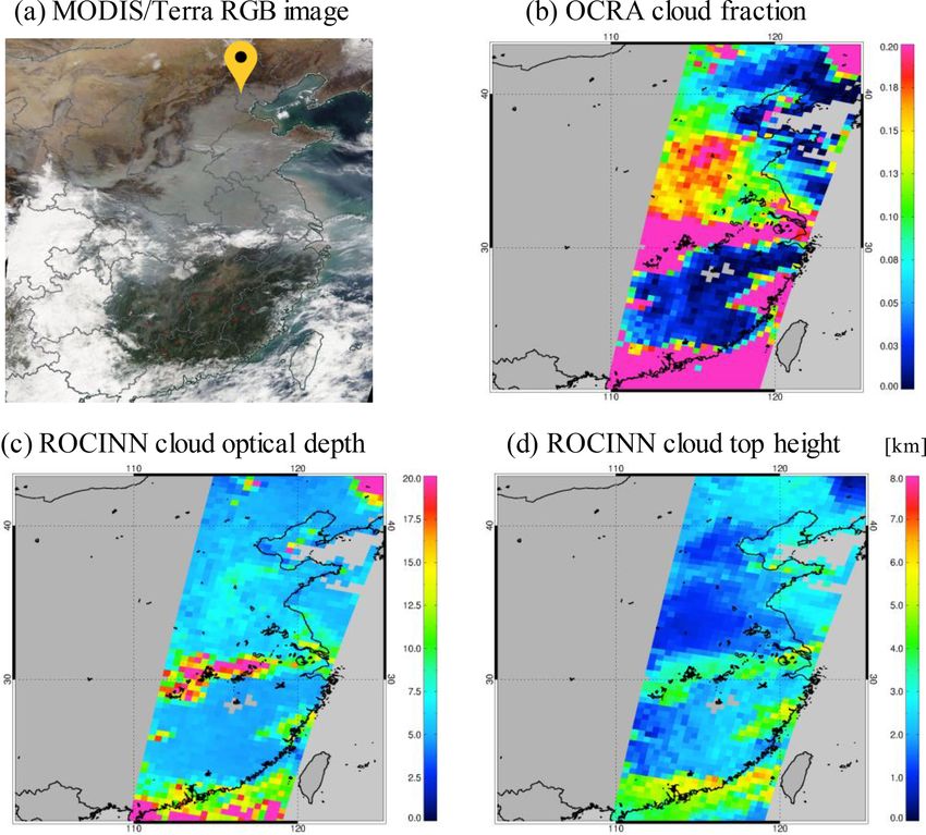
S. Liu et al.: An improved air mass factor calculation for NO2 measurements                                                                       759

Table 1. Ancillary parameters used to derive GOME-2 tropospheric NO2 columns. See Table 2 for details regarding the chemistry transport
models used to obtain the a priori NO2 profiles.

                                                       Reference retrieval (Liu et al., 2019b)     Improved algorithm (this work)
                        Surface albedo                 GOME-2 LER climatology                      GOME-2 direction-dependent LER
                        A priori NO2 profile           TM5-MP                                      IFS (CBA)
                        Cloud parameter                OCRA/ROCINN_CRB                             OCRA/ROCINN_CAL

Table 2. Summary of the chemistry transport model specifications.

                                               TM5-MP (Huijnen et al., 2010;                     IFS (CBA) (Flemming et al., 2015;
                                               Williams et al., 2017)                            Huijnen et al., 2016)
          Horizontal resolution                1◦ (latitude, longitude)                          ∼ 80 km (T255) or ∼ 0.7◦ (latitude, longitude)
          Vertical resolution                  34 layers (∼ 6 layers below 1.5 km)               1371 layers (∼ 12 layers below 1.5 km)
          Temporal resolution                  2 h archiving                                     1 h archiving
          Meteorological fields                ECMWF 3 h                                         ECMWF online (initialised with ERA5)
          Tropospheric chemistry               Modified CB05 (Williams et al., 2013)             Modified CB05 (Williams et al., 2013)
          Anthropogenic emission               MACCity (Granier et al., 2011)                    CAMS_GLOB_ANT v2.1 (Granier et al., 2019)
          Advection                            Slopes scheme (Russell and Lerner, 1981)          Semi-Lagrangian scheme as described in
                                                                                                 Temperton et al. (2001) and Hortal (2002)
          Convection                           ECMWF                                             Bechtold et al. (2014)
          Diffusion                            Holtslag and Boville (1993)                       Beljaars and Viterbo (1998)
        1 A total of 69 layers are employed in this study.

3     Improved AMF calculation                                                       each segment with a parabolic fit to parameterise the VZA
                                                                                     dependency. The main idea of this VZA-dependency param-
3.1     Surface albedo                                                               eterisation is to use the VZA as a proxy for observation ge-
                                                                                     ometry over land, as the solar zenith angle (SZA) and relative
The dependency of surface reflection on the incoming                                 azimuth angle (RAA) are nearly constant at a given latitude
and outgoing directions is mathematically described by the                           and, thus, have been captured in the original GOME-2 LER
BRDF (Nicodemus et al., 1992), which shows a “hot spot”                              dataset.
of increased reflectivity in the backward scattering directions                         For each GOME-2 measurement, the surface DLER
over rough surfaces like vegetation and a strong forward scat-                       αDLER is calculated as follows:
tering peak near “sun glint” geometries over smooth surfaces
                                                                                     αDLER = αLER + c0 + c1 × θ + c2 × θ 2 ,                      (4)
such as water. In this study, we account for the direction de-
pendency of surface albedo for the GOME-2 LER clima-                                 where VZA θ is positive on the western side of the orbit
tology by applying a directionally dependent LER (DLER)                              swath and negative on the eastern side of the orbit swath. c0 ,
dataset over land surfaces (see Sect. 3.1.1) and by imple-                           c1 , and c2 are parabolic fitting coefficients depending on lat-
menting an ocean surface albedo parameterisation over water                          itude, longitude, month, and wavelength. The nondirectional
surfaces (see Sect. 3.1.2).                                                          LER αLER is taken from the traditional GOME-2 LER clima-
                                                                                     tology. Note that no directionality is provided by the DLER
3.1.1    Over land                                                                   dataset over water (without sea ice cover), which is mainly
                                                                                     due to the dependency on parameters such as wind speed and
To account for the surface BRDF in our NO2 AMF calcu-                                chlorophyll concentration that can not be easily cast into cli-
lation over land, the surface reflectivity is described by a                         matology. Additionally, due to the strong solar and viewing
GOME-2 DLER dataset (Tilstra et al., 2019) that captures the                         angle dependency of specular reflection, changes in the solar
VZA dependency. Compared with the traditional GOME-2                                 position in the course of a month influence the albedo over
LER climatology (Tilstra et al., 2017), which is derived from                        water bodies much more than over land, and this influence is
a range of viewing angles (∼ 115◦ for GOME-2 measure-                                modelled and described in Sect. 3.1.2.
ments covering the directions from east to west), the GOME-                              Figure 1a–c show the traditional GOME-2 LER climatol-
2 DLER dataset is derived by dividing the range of view-                             ogy, the GOME-2 DLER dataset over land, and their differ-
ing angles into five segments and applying the same retrieval                        ences on 3 February and 5 August 2010. The DLER data
method as in the traditional GOME-2 LER determination for                            show a stronger increase – by ∼ 0.02 – for the western view-

www.atmos-meas-tech.net/13/755/2020/                                                                        Atmos. Meas. Tech., 13, 755–787, 2020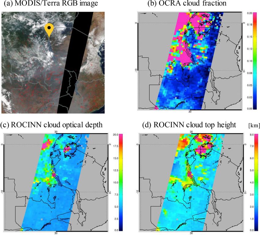
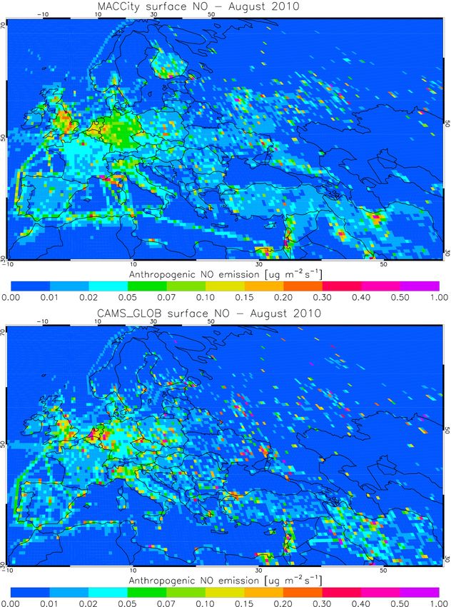
760                                           S. Liu et al.: An improved air mass factor calculation for NO2 measurements

Figure 1. Map of GOME-2 surface LER climatology (Tilstra et al., 2017) version 3.1 in February and August (a), improved GOME-2 surface
LER data taking the direction dependency on 3 February and 5 August 2010 into account (b), and their differences over land (c) and over
water (d). The improvements are described in Sect. 3.1.1 for land and in Sect. 3.1.2 for water.

ing direction over vegetation, ∼ 0.05 over desert, and ∼ 0.2          ice, due to the forward scattering peak or double scattering
over snow and ice, due to the increasing BRDF in the back-            peak in the BRDF pattern for snow (Dumont et al., 2010).
ward scattering direction. A slight change of up to 0.01 is           The difference in surface albedo is generally larger in winter
found over vegetation and desert with an enhancement in the           due to the change in surface conditions and/or sun elevation,
central part of the orbit swath and a reduction on the eastern        with the exception of desert areas.
side of the orbit swath. This effect is larger over snow and

Atmos. Meas. Tech., 13, 755–787, 2020                                                     www.atmos-meas-tech.net/13/755/2020/
S. Liu et al.: An improved air mass factor calculation for NO2 measurements                                                    761

Figure 2. Comparison of GOME-2 LER climatology (Tilstra et al., 2017) and GOME-2 DLER data (a) and the impact on the clear-sky
AMFs (b) over western Europe (44–53◦ N, 0–7◦ E) and eastern China (21–41◦ N, 110–122◦ E) as a function of VZA in February 2010
(VZAs are negative for observations on the eastern side of the orbit swath).

   Figure 2 compares the surface LER and DLER as a                 2018; Qin et al., 2019). With a good agreement with the es-
function of VZA and presents the impact on the clear-sky           tablished MODIS BRDF product (Tilstra et al., 2019), both
AMFs over western Europe (44–53◦ N, 0–7◦ E) and eastern            in the absolute sense and in the directional/angular depen-
China (21–41◦ N, 110–122◦ E) in February 2010. The sur-            dency, the GOME-2 DLER dataset is derived from mea-
face albedo on the western side of the orbit swath (backward       surements of the instrument itself, which is consistent with
scattering direction) is higher by up to 0.024 for both regions,   the GOME-2 NO2 observations, considering the illumination
which increases the calculated clear-sky AMFs by 9 %–14 %.         conditions, observation geometry, and instrumental charac-
Smaller differences (by up to 0.006) are found for the cen-        teristics; therefore, the use of GOME-2 DLER introduces no
tral and eastern viewing directions for surface albedo and for     additional bias caused by the instrumental differences.
clear-sky AMFs (by up to 4 %).
   Figure 3 shows the differences in tropospheric NO2              3.1.2   Over water
columns retrieved using the surface LER and DLER datasets
for a given day and for the monthly average in February            The surface reflectivity over water is described with im-
and August 2010. The daily differences in the tropospheric         proved GOME-2 LER data using an ocean surface albedo
NO2 columns are consistent with Fig. 1c, with a larger im-         parameterisation (Jin et al., 2004, 2011) to account for the
pact found over polluted regions. Taking Spain on 3 Febru-         direction dependency. Based on atmospheric radiation mea-
ary 2010 as an example, the approximately 0.005 smaller            surements and the Coupled Ocean and Atmosphere Radia-
surface DLER in the central part of the orbit swath results        tive Transfer (COART) model (Jin et al., 2006), the param-
in a lower sensitivity to tropospheric NO2 columns in the          eterisation developed by Jin et al. (2011) derives the surface
AMF calculation; therefore, the AMF decreases and the tro-         reflectivity for the direct (sun) and diffuse (sky) incident ra-
pospheric NO2 columns increases by ∼ 1×10¹⁴ molec. cm−2            diation separately and further divides each of them into con-
(3 %). In contrast, the surface DLER is approximately 0.02         tributions from surface and water respectively. This parame-
higher on the western side of the orbit swath over eastern         terisation has been used to derive ocean surface albedo (e.g.
China on the same day; thus, the tropospheric NO2 column           Séférian et al., 2018) and to generate satellite NO2 products
is approximately 3 × 10¹⁵ molec. cm−2 (11 %) lower. The            (e.g. Laughner et al., 2018).
monthly differences in the tropospheric NO2 columns show a            Following Jin et al. (2011), the ocean surface albedo αtotal
larger reduction in winter: by more than 5×10¹⁴ molec. cm−2        is defined as follows:
over regions such as central Europe, South Africa, India,                          s      w              s      w
                                                                   αtotal = fdir (αdir + αdir ) + fdif (αdif + αdif ),          (5)
and eastern China, and by ∼ 1 × 10¹⁴ molec. cm−2 over ar-
eas such as the eastern US, Southeast Asia, and Mexico.            where αdir s and α s are the respective direct and diffuse
                                                                                       dif
   Accounting for the BRDF effect, the surface DLER cap-           contribution of the surface reflection, and αdir  w and α w are
                                                                                                                             dif
tures the cross-track dependency of surface albedo, such as        the respective direct and diffuse contribution of the volume
the increased reflectivity in the backward scattering viewing      scattering of water below the surface. The respective di-
geometries, which is in agreement with studies that have ap-       rect and diffuse fraction of downward surface flux, fdir and
plied the BRDF product from MODIS to describe the depen-           fdif (fdif = 1 − fdir ), are calculated using the online COART
dency of land surface reflectance on illumination and view-        model (https://satcorps.larc.nasa.gov/jin/coart.html, last ac-
ing geometry (e.g. Zhou et al., 2010; Noguchi et al., 2014;        cess: 12 February 2020). The direct surface albedo αdir       s ,
Vasilkov et al., 2017; Lorente et al., 2018; Laughner et al.,      which is one main component of the total ocean surface

www.atmos-meas-tech.net/13/755/2020/                                                      Atmos. Meas. Tech., 13, 755–787, 2020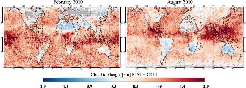
762                                            S. Liu et al.: An improved air mass factor calculation for NO2 measurements

Figure 3. Differences in the GOME-2 tropospheric NO2 columns retrieved using the GOME-2 LER and DLER datasets for a given day and
for the monthly average in February and August 2010. Only measurements with a cloud radiance fraction less than 0.5 are included.

albedo, describes the contribution of Fresnel reflection de-
pending on the incident angle, the refractive index of seawa-
ter (1.343 at 460 nm), and the slope distribution of the ocean
surface (defined by Cox and Munk (1954) and related to a
wind speed of 5 m s−1 from the climatological mean). The
diffuse surface albedo αdifs is difficult to formulate analyti-

cally due to its variation with atmospheric conditions; thus,
it is parameterised practically to be 0.06 for an assumed wind
speed of 5 m s−1 . The direct water volume albedo αdir  w is con-

sidered for Case 1 waters (open ocean waters dominated by
phytoplankton and associated products that comprise 99 % of
the ocean) and is primarily affected by the chlorophyll con-
centration (0.2 mg m−3 from the global ocean average). The
diffuse water volume albedo αdif w is defined by the α w at an
                                                         dir         Figure 4. Parameterised ocean surface albedo for a non-glint con-
effective incident direction, i.e. arccos(0.676), and is calcu-      dition and its albedo components due to direct and diffuse surface
lated to be 0.0145. The direct fraction of downward surface          reflection and direct and diffuse water volume scattering as a func-
flux fdir is calculated using a radiative transfer simulation        tion of incident angle.
with a mid-latitude summer atmosphere, a marine aerosol op-
tical depth of 1 (at 550 nm), and a 100 m ocean depth with the
average Petzold phase function for ocean particle scattering.
                                                                     dent angles (below 55◦ ) and higher values for larger incident
    Figure 4 shows the parameterised ocean surface albedo for
                                                                     angles. The relative contribution of the diffuse component
a non-glint situation as well as its four albedo components
                                                                     to the total ocean surface albedo fdif increases from ∼ 0.65
as a function of incident angle. The overall shape of the total
                                                                     to ∼ 1 with incident angle. It is worth noting that the four
ocean surface albedo αtotal is dependent on the incident angle
                                                                     albedo components are independent of each other and are,
with a peak near 70◦ , which is similar to Jin et al. (2004) and
                                                       s + αs )      thus, flexible to update or replace.
Laughner et al. (2018). The surface component (αdir            dif
                                                 w       w ), par-      Based on measurements over a long period (2007–2018
is larger than the water volume component (αdir + αdif
                                                                     for version 3.1), the GOME-2 LER climatology mainly pro-
ticularly for larger incident angles. The direct component                                             s + α w ) over water bodies
    s + α w ) increases with incident angle and has lower val-       vides the diffuse component (αdif       dif
(αdir     dir
                                     s + α w ) for smaller inci-     with minimised impact of direct contribution. Therefore, we
ues than the diffuse component (αdif        dif                                                               s + α w in Jin et al.
                                                                     replace the simplified expression of αdif      dif

Atmos. Meas. Tech., 13, 755–787, 2020                                                     www.atmos-meas-tech.net/13/755/2020/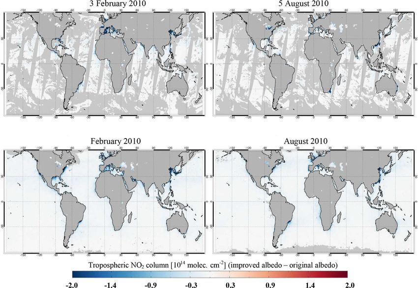
S. Liu et al.: An improved air mass factor calculation for NO2 measurements 763
(2011) with values taken from the GOME-2 LER clima- spacing of ∼ 80 km globally (∼ 0.7◦ ). The model is run with
tology. This scheme enables the consideration of the direc- the standard 137 hybrid sigma-pressure layers as also used
tion dependency for the GOME-2 LER climatology over wa- operationally in the forecast and reanalysis model from the
ter with minimal bias introduced. In addition, most of the ECMWF. From this, we select a vertical discretisation based
ocean surface albedo studies (e.g. Ohlmann, 2003; Jin et al., on 69 vertical levels up to 0.1 hPa with ∼ 12 layers in the
2004, 2011; Li et al., 2006; Laughner et al., 2018) employ boundary layer for further processing. An essential differ-
a straightforward assumption that the SZA is the only di- ence compared with TM5-MP is that the chemistry is an inte-
rectional parameter involved in the parameterisation, specif- gral part of the meteorological forecast model in IFS (CBA).
ically the incident angle is assumed to be equivalent to the Here we use the forecast model from cycle 45r2, which is
SZA in the Fresnel reflection calculation. In this work, we initialised daily using ERA5 meteorology. Additionally, an-
apply the full equation to derive the local incident angle thropogenic emissions are based on the recently prepared
that also considers the dependencies on VZA and RAA, and CAMS_GLOB_ANT v2.1 emission inventory (Granier et al.,
we additionally implement the Cox–Munk sun glitter model 2019), as illustrated in Appendix A, and day-specific biomass
over glint-contaminated regions. See Cox and Munk (1954) burning emissions are taken from GFASv2.1 (Kaiser et al.,
and Gordon (1997) for more details on the configuration and 2012). The NO2 data are available on an hourly basis, with
derivation. profiles at the satellite measurement time obtained by linear
Figure 1b and d present the calculated ocean surface interpolation.
albedo and the differences with respect to values taken Figure 6 shows an intercomparison of area-averaged and
from GOME-2 LER climatology on 3 February and 5 Au- monthly averaged profiles from TM5-MP and IFS (CBA)
gust 2010. Consistent with Vasilkov et al. (2017), the im- at the GOME-2 overpass time (09:30 LT) over western Eu-
proved ocean surface albedo shows up to 0.015 higher values rope (44–53◦ N, 0–7◦ E) and eastern China (21–41◦ N, 110–
at larger SZAs and VZAs, where the higher incident angles 122◦ E) in February and August 2010. Generally, TM5-MP
result in stronger Fresnel reflections, and up to 0.025 higher and IFS (CBA) show similar mean profile shapes over the
values over areas affected by sun glint, which is typically the two regions. In February, IFS (CBA) shows a larger bound-
eastern swath of GOME-2 orbits. ary layer concentration and a sharper transition to the free
Figure 5 shows the impact of using updated ocean sur- troposphere over western Europe and larger NO2 gradients
face albedo on our GOME-2 NO2 retrieval for a given day in the free troposphere over eastern China. In August, the
and for the monthly average in February and August 2010. NO2 concentrations in the free troposphere are lower than in
The tropospheric NO2 columns are mainly reduced over the February for both models due to the reduced emissions and
polluted coastal regions that have large NO2 concentrations the reduced lifetime of NO2 , and a larger surface layer NO2
and for large SZAs and VZAs. For instance, the ocean sur- gradient is found for the IFS (CBA) model for both regions.
face albedo around Spain increases by ∼ 0.01 on 3 Febru- Figure 7 shows the daily TM5-MP and IFS (CBA) a pri-
ary 2010, leading to a decrease in the tropospheric NO2 ori NO2 profiles over the Netherlands (52.8◦ N, 4.7◦ E) and
columns by up to 8 × 10¹⁴ molec. cm−2 (9 %). The monthly China (39.1◦ N, 118.0◦ E) on 3 February 2010 as examples.
average of the tropospheric NO2 columns decreases in win- IFS (CBA) shows a higher surface layer NO2 concentra-
ter by more than 3 × 10¹⁴ molec. cm−2 near the coastal area, tion (a steeper profile shape) and yields a tropospheric AMF
e.g. around the US, eastern China, and Brazil, and by up to that is reduced by 0.21 over the Netherlands, which will en-
1 × 10¹⁴ molec. cm−2 along the shipping lanes, e.g. in the hance the retrieved tropospheric NO2 column. In contrast,
Mediterranean Sea, the Red Sea, and maritime Southeast the tropospheric AMF increases by 0.06 over China due to
Asia. the larger NO2 gradients in the free troposphere (a less steep
profile shape) modelled by IFS (CBA).
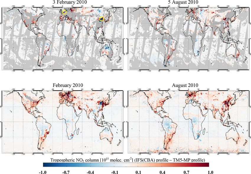
3.2 A priori NO2 profile Figure 8 shows the differences in the tropospheric NO2
columns retrieved using TM5-MP and IFS (CBA) a pri-
In regions with strong gradients with respect to NOx emis- ori NO2 profiles for a given day and for the monthly av-
sions in space and time, the significant variation of surface erage in February and August 2010. The differences are
NO2 can only be captured in a model with sufficient hori- consistent with the changes in the profile shapes in Figs. 6
zontal, vertical, and temporal resolution. The advanced IFS and 7. The use of IFS (CBA) generally increases the tro-
(CBA) (Huijnen et al., 2016, 2019) global chemistry fore- pospheric NO2 columns over polluted regions, e.g. over
cast and analysis system combines the stratospheric chem- western Europe, the eastern US, and Argentina, by up to
istry scheme developed for the Belgian Assimilation Sys- 2 × 10¹⁵ molec. cm−2 and decreases the values over areas
tem for Chemical ObsErvations (BASCOE, Skachko et al., such as central Africa, South Africa, and Brazil, by up to
2016) and the modified CB05 tropospheric chemistry scheme 1 × 10¹⁵ molec. cm−2 . In February, however, a strong en-
(Williams et al., 2013). As summarised in Table 2, the spa- hancement of ∼ 7 × 10¹⁵ molec. cm−2 is found over north-
tial resolution of IFS (CBA) is a reduced Gaussian grid at ern Germany and Poland, and a strong reduction of ∼ 4 ×
a spectral truncation of T255, which is equivalent to a grid 1015 molec. cm−2 is found over the North China Plain. The
www.atmos-meas-tech.net/13/755/2020/ Atmos. Meas. Tech., 13, 755–787, 2020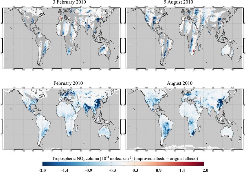
764                                           S. Liu et al.: An improved air mass factor calculation for NO2 measurements

Figure 5. Differences in the GOME-2 tropospheric NO2 columns retrieved using the original GOME-2 LER climatology and the GOME-2
LER data improved by the ocean surface albedo parameterisation for a given day and for the monthly average in February and August 2010.
Only measurements with a cloud radiance fraction less than 0.5 are included.

Figure 6. Area-averaged and monthly averaged profiles from TM5-MP and IFS (CBA) at the GOME-2 overpass time (09:30 LT) over western
Europe (44–53◦ N, 0–7◦ E) and eastern China (21–41◦ N, 110–122◦ E) in February and August 2010.

differences in Fig. 8 are likely related to the different trans-      et al., 2018; Liu et al., 2019b). Figure 7 compares the IFS
port scheme and emission inventories employed by the model            (CBA) a priori NO2 profiles to original and different model
as well as the different model resolutions.                           resolutions over the Netherlands (52.8◦ N, 4.7◦ E) and China
   To quantify the effect of model resolution, a more detailed        (39.1◦ N, 118.0◦ E) on 3 February 2010. Both examples are
analysis was implemented for IFS (CBA) that used 1◦ grids             located in polluted coastal regions that typically have a large
for the horizontal resolution, 34 layers for the vertical reso-       heterogeneity and variability in the NO2 distribution. The
lution, and a 2 h time step for the temporal resolution. These        AMFs differ by more than 0.02 for both example locations
values are of the same order of magnitude as the model res-           due to differences in the horizontal and vertical resolutions.
olution of TM5-MP and other chemistry transport models                The current 2 h temporal sampling and subsequent linear in-
currently employed in the satellite retrieval of global NO2           terpolation between the sampling points is sufficient for the
(e.g. van Geffen et al., 2019; Lorente et al., 2017; Boersma          retrieval of tropospheric NO2 columns (not shown). When

Atmos. Meas. Tech., 13, 755–787, 2020                                                     www.atmos-meas-tech.net/13/755/2020/
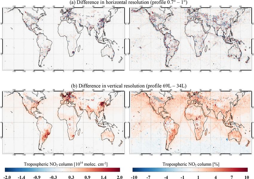
S. Liu et al.: An improved air mass factor calculation for NO2 measurements                                                          765

Figure 7. A priori NO2 profiles from TM5-MP, IFS (CBA) (original resolution), and IFS (CBA) with different model resolutions over the
Netherlands (52.8◦ N, 4.7◦ E) and China (39.1◦ N, 118.0◦ E) on 3 February 2010. The IFS (CBA) profiles for a 1◦ grid and for 34 layers are
compared. The calculated clear-sky tropospheric AMF is given next to each label in the legends.

Figure 8. Differences in tropospheric NO2 columns retrieved using TM5-MP and IFS (CBA) a priori NO2 profiles for a given day and
for the monthly average in February and August 2010. Yellow circles in the top-left panel indicate the locations utilised in Fig. 7. Only
measurements with a cloud radiance fraction less than 0.5 are included.

a coarser spatial resolution is used, the “domain-averaged”               Figure 9 shows the absolute and relative differences in
profiles generally show an increased surface NO2 concentra-            tropospheric NO2 columns retrieved by altering the model
tion for the unpolluted domain and the opposite for the emis-          resolutions for IFS (CBA) a priori NO2 profiles in Febru-
sion source. Consequently, the AMF is underestimated for               ary 2010. In Fig. 9a, the increase in the spatial resolution
unpolluted areas and overestimated for polluted areas. When            (1◦ vs. 0.7◦ grid) changes the tropospheric NO2 columns
the number of layers is reduced, the coarser sampling points           by up to 7 × 10¹⁴ molec. cm−2 or 20 % for polluted regions,
can not accurately capture the large NO2 gradients at low              confirming the importance of applying a priori NO2 pro-
altitudes, particularly for polluted regions where the mea-            files with better spatial resolution (Heckel et al., 2011; Lin
surement sensitivity of the satellite decreases significantly          et al., 2014; Kuhlmann et al., 2015). Larger relative dif-
towards the surface.                                                   ferences are observed over cities surrounded by rural ar-

www.atmos-meas-tech.net/13/755/2020/                                                         Atmos. Meas. Tech., 13, 755–787, 2020
766                                            S. Liu et al.: An improved air mass factor calculation for NO2 measurements

eas, coastal regions, isolated islands, and shipping lanes,          2015), which can be considered to be a reflectance-weighted
where the use of high spatial resolutions more accurately            height located inside a cloud. Additionally, as the enhanced
captures the NO2 emissions and chemistry for a priori pro-           multiple scattering is not fully taken into account in the CRB-
files. In Fig. 9b, the improvement in the vertical resolution        based cloud retrieval, the retrieved cloud height is normally
(34 vs. 69 layers) enhances the tropospheric NO2 columns             close to the altitude of the middle.
by up to 5 × 10¹⁴ molec. cm−2 or 15 %. Increasing the num-              In Fig. 10, higher cloud top heights are mainly found over
ber of layers generally better resolves the NO2 vertical vari-       land surfaces characterised by the presence of a large amount
ation, especially for the lowest model layers where the box-         of absorbing aerosols when using CRB, i.e. over regions
AMF decreases significantly in the polluted cases. Conse-            with strong desert dust emissions, such as the Sahara, the
quently, the tropospheric AMFs are lower and the tropo-              Arabian Desert, and the deserts in Australia, as well as re-
spheric NO2 columns are higher for polluted regions (Heckel          gions with strong biomass burning emissions, such as South
et al., 2011; Russell et al., 2011; Valin et al., 2011). For un-     America, South Africa, and Southeast Asia. Over these areas,
polluted regions, the differences are generally small (within        ROCINN likely retrieves an effective aerosol height close to
±2 × 10¹⁴ molec. cm−2 or ±3 %). In addition, the use of dif-         the top of aerosol layer, depending on the type of absorb-
ferent temporal resolution (a 2 h vs. a 1 h time step) generally     ing aerosols and on the aerosol optical depth. The presence
has a negligible impact on the tropospheric NO2 columns              of strongly absorbing aerosols, which typically have large
(less than 2 × 10¹⁴ molec. cm−2 or 3 %, not shown).                  aerosol optical depth and/or are located at high altitudes (up
                                                                     to ∼ 8 km), reduces the fraction of photons reaching the low-
3.3   Cloud correction                                               est part of the atmosphere. In order to approximate this short-
                                                                     ened light path, the CRB-based cloud retrieval has to put the
For cloudy scenarios, the retrieval of tropospheric NO2 is af-       Lambertian reflector at a higher altitude (Wang et al., 2012;
fected by the cloud parameters due to the variation in scene         Chimot et al., 2016). This effect is larger for aerosol lay-
albedo and the photon path redistribution in the troposphere.        ers at higher altitudes and is also dependent on geometry
As described in Sect. 2, the cloudy-sky AMFs are calcu-              parameters like SZA, on surface properties such as surface
lated by the independent pixel approximation using GOME-             albedo, and on the accuracy of radiometric cloud fractions
2 cloud parameters: radiometric cloud fraction from OCRA             from OCRA. See Sect. 4 for further discussion on the CRB
as well as cloud top pressure (cloud top height) and cloud           and CAL cloud models in the presence of aerosols.
albedo (cloud optical depth) from ROCINN. To improve                    To apply the CAL cloud model in our NO2 AMF calcu-
the cloud correction in our NO2 retrieval, the CAL model             lation, a single scattering albedo of 1 and an asymmetry pa-
from the ROCINN cloud algorithm (Loyola et al., 2018),               rameter of 0.85 for water clouds are assumed for the radiative
where the clouds are treated as optically uniform layers of          transfer calculation; these values are consistent with those
light-scattering water droplets, is applied. The CAL model is        used in the cloud retrieval (Loyola et al., 2018). Cloud ob-
more representative of the real situation than the CRB model         servations with a fitting root mean square (rms) greater than
(where the clouds are idealised as Lambertian reflectors with        1 × 10⁻⁴ or a number of iterations greater than 20 are fil-
zero transmittance), as it allows the penetration of photons         tered out. The NO2 box-AMFs are derived through the pixel-
through the cloud layer. This treatment takes the multiple           specific radiative transfer calculation instead of the interpo-
scattering of light inside the cloud and the contribution of the     lation from a LUT with fixed reference points. This requires
atmospheric layer between the cloud bottom and the ground            no projection from the layer coordinate of the NO2 profile
into account.                                                        to the coordinate assumed in the LUT and also requires no
   Figure 10 shows the differences in cloud top heights ob-          linear interpolation based on the model parameters.
tained with the CRB and CAL models from GOME-2 mea-                     Figure 11 shows an example of the box-AMFs derived for
surements in February and August 2010. Consistent with               clear and cloudy sky using the CRB and CAL models over
Loyola et al. (2018) (see Figs. 3 and 13 therein), the cloud top     Italy (45.3◦ N, 11.2◦ E) on 1 February 2010. The cloud in-
heights from CAL are generally higher by ∼ 0.9 km on aver-           formation and the calculated tropospheric AMFs are also re-
age. Stronger increases (up to 2 km) are found over regions          ported. Compared with the clear-sky box-AMFs, the CAL-
with thick and high clouds, such as the Intertropical Conver-        based cloudy-sky box-AMFs increase above the cloud layer
gence Zone and the Western Hemisphere Warm Pool, which               (albedo effect) and decrease below the cloud layer (shielding
is very similar to the findings of Lelli et al. (2012; see Fig. 12   effect). Compared with the CRB model, the use of the CAL
therein). In general, the CRB-based cloud retrieval underes-         model considers the sensitivities inside and below the cloud
timates the cloud top height due to the neglect of oxygen ab-        layer and increases the cloudy-sky AMF by 0.3, which con-
sorption throughout a cloud layer (Vasilkov et al., 2008) and,       sequently decreases the retrieved tropospheric NO2 column
thus, the misinterpretation of the smaller top-of-atmosphere         by 2.5×10¹⁵ molec. cm−2 (12 %), based on the polluted NO2
reflectance as a lower cloud layer (Saiedy et al., 1967). The        profile with most of the NO2 concentration located near the
retrieved cloud height is normally close to the middle, i.e. the     surface.
optical centroid of clouds (Ferlay et al., 2010; Richter et al.,

Atmos. Meas. Tech., 13, 755–787, 2020                                                   www.atmos-meas-tech.net/13/755/2020/
S. Liu et al.: An improved air mass factor calculation for NO2 measurements 767
Figure 9. Absolute and relative differences in the tropospheric NO2 columns retrieved by altering the model resolutions for IFS (CBA) a
priori NO2 profiles in February 2010. The tropospheric NO2 columns are compared for a 1 and 0.7◦ grid (a) and for 34 and 69 layers (b).
Only measurements with a cloud radiance fraction less than 0.5 are included.
Figure 10. Differences in cloud top heights retrieved using the ROCINN_CAL and ROCINN_CRB cloud models in February and Au-
gust 2010. Only measurements with a cloud fraction less than 0.3 are included. Observations with a fitting rms greater than 1 × 10⁻⁴ or a
number of iterations greater than 20 are filtered out.
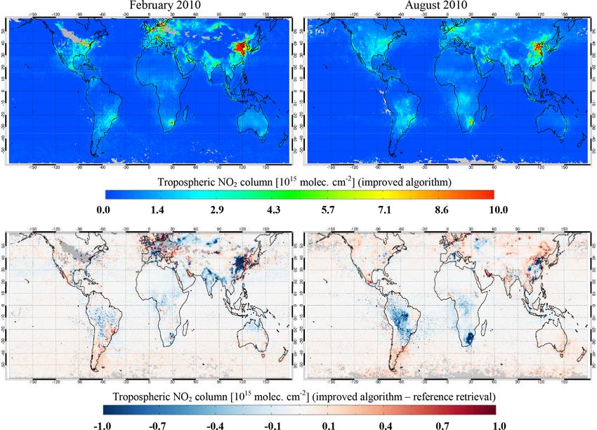
Figure 12 shows the differences in the tropospheric NO2 3.4 Combined impact
columns retrieved using the CRB and CAL models in Febru-
ary and August 2010. The use of the CAL model de-
creases the tropospheric NO2 columns by more than 1 ×
1014 molec. cm−2 over polluted regions. Larger values are Figure 13 shows the tropospheric NO2 columns retrieved us-
found in winter (up to 3 × 10¹⁵ molec. cm−2 ), when most ing the improved AMF calculation and the differences from
of the NO2 concentrations are located at the surface and the the reference data in February and August 2010. Larger dif-
cloud fractions are generally larger due to the seasonal vari- ferences are found in winter over the polluted regions. For
ation of clouds. instance, the tropospheric NO2 columns are reduced by more
than 1 × 10¹⁵ molec. cm−2 over China and India in February
as well as Brazil and South Africa in August. Increased val-
www.atmos-meas-tech.net/13/755/2020/ Atmos. Meas. Tech., 13, 755–787, 2020768 S. Liu et al.: An improved air mass factor calculation for NO2 measurements
corrected implicitly in the AMF calculation via the effective
cloud parameters (i.e. aerosols are treated as clouds).
Figures 14 and 15 show the land surface RGB image
with active fire locations from the Moderate Resolution
Imaging Spectroradiometer (MODIS) on board the Terra
(10:30 LT) and the OCRA/ROCINN cloud products mea-
sured by GOME-2 (09:30 LT) over eastern China and cen-
tral Africa on a given day respectively. The MODIS dataset
(https://worldview.earthdata.nasa.gov/, last access: 12 Febru-
ary 2020) describes the cloud or aerosol amount and fire lo-
cations (for central Africa). For both regions, large aerosol
loads are found in the RGB image for cloud-free areas, such
as the Beijing–Tianjin–Hebei economic region in eastern
Figure 11. The box-AMFs for clear and cloudy sky using China and burning regions across central Africa, where the
the ROCINN_CAL and ROCINN_CRB cloud models over Italy aerosol loads are identified as thin clouds (a cloud optical
(45.3◦ N, 11.2◦ E) on 1 February 2010. The tropospheric AMF is depth of ∼ 5) near the surface (a cloud top height of ∼ 3 km)
given next to each label. The ROCINN_CRB cloud top pressure with cloud fractions of up to 0.18.
is shown as a green horizontal dotted line, and the ROCINN_CAL Therefore, we assume that the thin clouds near the sur-
cloud top and base pressures are shown as brown horizontal dotted
face in the OCRA/ROCINN cloud products are attributed to
lines. The cloud radiance fraction is 0.47, the cloud optical depth is
6.85, the SZA is 69◦ , the VZA is 3◦ , and the RAA is 42◦ .
aerosol loads for measurements with a cloud radiance frac-
tion less than 0.5 or a cloud fraction less than 0.2, and we
evaluate the accuracy of the implicit aerosol correction by
comparing it with the explicit aerosol correction. For this pur-
ues are found over regions such as Mexico, Argentina, and
pose, the explicit correction for aerosols is implemented us-
Russia.
ing ground-based aerosol observations at Xianghe (39.75◦ N,
Table 3 summarises the individual changes and the com-
116.96◦ E), which is a suburban site surrounded by heav-
bined effect of our improved AMF calculation on the re-
ily industrialised areas in northeastern China (Clémer et al.,
trieved tropospheric NO2 columns over western Europe,
2010; Hendrick et al., 2014; Vlemmix et al., 2015), and at
eastern China, the eastern US, and central Africa. Increases
Bujumbura (3.38◦ S, 29.38◦ E), which is located in the cen-
in the GOME-2 surface albedo reduce the tropospheric NO2
tral African country of Burundi and surrounded by intensive
columns by 2 %–6 %. The use of IFS (CBA) a priori NO2
biomass burning activities (Gielen et al., 2017), as indicated
profiles affects (mostly increases) the tropospheric NO2
in Figs. 14 and 15 respectively. Our analysis is further lim-
columns by up to 21 %, and the use of CAL cloud parameters
ited to satellite measurements with a cloud optical depth less
decreases the values by up to 14 %. The combined effect of
than 5 and a cloud top height less than 3 km to reduce the
individual improvements yields to an average change in the
cloud contamination. With this selection, the aerosol con-
tropospheric NO2 columns of within ±15 % in winter and
centrations are generally low or moderate (an aerosol optical
±5 % in summer over polluted regions.
depth less than 1).
The uncertainty in the improved AMF calculation is likely
The explicit modelling of aerosol scattering and absorp-
reduced relative to the reference retrieval if the improved sur-
tion for the AMF calculation is implemented by introducing
face albedo dataset, a priori NO2 profiles, and cloud parame-
the aerosol optical properties (i.e. single scattering albedo
ters are considered, as they are the main causes of AMF un-
and phase function) and vertical distributions (i.e. extinction
certainty (Lorente et al., 2017). The uncertainty in the AMF
vertical profiles) into the radiative transfer calculation. The
calculation for polluted conditions is estimated to have im-
single scattering albedo describes the fraction of the aerosol
proved from 10 % to 45 % for the reference retrieval to be-
light scattering over the extinction, and the phase function
tween 10 % and 35 % in this work.
describes the angular distribution of the scattered light in-
tensity. In this study, we apply the Henyey–Greenstein phase
function with an asymmetry parameter (the first moment of
4 Implicit aerosol correction phase function) describing the asymmetry between forward
and backward scattering. The long-term statistics of the sin-
Aerosols can increase or decrease the sensitivity to tropo- gle scattering albedo and the asymmetry parameter at 440 nm
spheric NO2 , depending on the NO2 and aerosol vertical dis- are derived for Xianghe and Bujumbura using the Version 3
tribution as well as the optical and physical properties of Level 2.0 inversion products from the sun photometer radi-
the particles (Martin et al., 2003; Leitão et al., 2010). As ance measurements from AERONET (Holben et al., 1998;
the OCRA/ROCINN cloud retrieval does not distinguish be- Giles et al., 2019) (http://aeronet.gsfc.nasa.gov/, last access:
tween clouds and aerosols, the aerosol effect is assumed to be 12 February 2020). Monthly mean parameters are calcu-
Atmos. Meas. Tech., 13, 755–787, 2020 www.atmos-meas-tech.net/13/755/2020/You can also read