Development and testing scenarios for implementing land use and land cover changes during the Holocene in Earth system model experiments - Geosci ...
←
→
Page content transcription
If your browser does not render page correctly, please read the page content below
Geosci. Model Dev., 13, 805–824, 2020
https://doi.org/10.5194/gmd-13-805-2020
© Author(s) 2020. This work is distributed under
the Creative Commons Attribution 4.0 License.

Development and testing scenarios for implementing
land use and land cover changes during the Holocene
in Earth system model experiments
Sandy P. Harrison1 , Marie-José Gaillard2 , Benjamin D. Stocker3,4 , Marc Vander Linden5 , Kees Klein Goldewijk6,7 ,
Oliver Boles8 , Pascale Braconnot9 , Andria Dawson10 , Etienne Fluet-Chouinard11 , Jed O. Kaplan12,13 ,
Thomas Kastner14 , Francesco S. R. Pausata15 , Erick Robinson16 , Nicki J. Whitehouse17 , Marco Madella18,19,20 , and
Kathleen D. Morrison8
1 Department    of Geography and Environmental Science, University of Reading, Reading, UK
2 Department    of Biology and Environmental Science, Linnaeus University, Kalmar, Sweden
3 Ecological and Forestry Applications Research Centre, Cerdanyola del Vallès, Spain
4 Department of Earth System Science, Stanford University, Stanford, CA 94305, USA
5 Department of Archaeology, University of Cambridge, Cambridge, UK
6 PBL Netherlands Environmental Assessment Agency, the Hague, the Netherlands
7 Copernicus Institute of Sustainable Development, Utrecht University, Utrecht, the Netherlands
8 University Museum of Archaeology & Anthropology, University of Pennsylvania, Philadelphia, USA
9 Laboratoire des Sciences du Climat et de l’Environnement, Gif-sur-Yvette, France
10 Department of General Education, Mount Royal University, Calgary, Canada
11 Department of Earth System Science, Stanford University, Stanford, California, USA
12 Department of Earth Sciences, University of Hong Kong, Hong Kong
13 Institute of Geography, University of Augsburg, Augsburg, Germany
14 Senckenberg Biodiversity and Climate Research Centre, Frankfurt am Main, Germany
15 Centre ESCER, Department of Earth and Atmospheric Sciences, University of Quebec in Montreal, Montreal, Canada
16 Department of Anthropology, University of Wyoming, Laramie, Wyoming, USA
17 School of Geography, Earth and Environmental Science, University of Plymouth, Plymouth, UK
18 Department of Humanities (CaSEs), University Pompeu Fabra, Barcelona, Spain
19 ICREA Passeig Lluís Companys 23, 08010 Barcelona, Spain
20 School of Geography, Archaeology and Environmental Studies, University of the Witwatersrand,

Johannesburg, South Africa

Correspondence: Sandy P. Harrison (s.p.harrison@reading.ac.uk)

Received: 5 May 2019 – Discussion started: 23 July 2019
Revised: 12 January 2020 – Accepted: 20 January 2020 – Published: 2 March 2020

Abstract. Anthropogenic changes in land use and land          Changes (PAGES) LandCover6k initiative is working to-
cover (LULC) during the pre-industrial Holocene could have    wards improved reconstructions of LULC globally. In this
affected regional and global climate. Existing scenarios of   paper, we document the types of archaeological data that are
LULC changes during the Holocene are based on rela-           being collated and how they will be used to improve LULC
tively simple assumptions and highly uncertain estimates      reconstructions. Given the large methodological uncertain-
of population changes through time. Archaeological and        ties involved, both in reconstructing LULC from the archae-
palaeoenvironmental reconstructions have the potential to     ological data and in implementing these reconstructions into
refine these assumptions and estimates. The Past Global       global scenarios of LULC, we propose a protocol to evaluate

Published by Copernicus Publications on behalf of the European Geosciences Union.
806          S. P. Harrison et al.: Development and testing scenarios for implementing land use and land cover changes

the revised scenarios using independent pollen-based recon-        regions with no major local human activity (Vavrus et al.,
structions of land cover and climate. Further evaluation of the    2008; Pongratz et al., 2010; He et al., 2014; Smith et al.,
revised scenarios involves carbon cycle model simulations          2016). At the global scale, the biogeophysical effects of the
to determine whether the LULC reconstructions are consis-          accumulated LULC change during the Holocene, which re-
tent with constraints provided by ice core records of CO2          sulted in reconstructed land cover patterns in 1850 CE, have
evolution and modern-day LULC. Finally, the protocol out-          been estimated to cause a slight cooling (0.17 ◦ C) that is off-
lines how the improved LULC reconstructions will be used           set by biogeochemical warming (0.9 ◦ C), giving a net global
in palaeoclimate simulations in the Palaeoclimate Modelling        warming (0.73 ◦ C) (He et al., 2014). However, in these simu-
Intercomparison Project to quantify the magnitude of anthro-       lations, biophysical and biogeochemical effects were of com-
pogenic impacts on climate through time and ultimately to          parable magnitude in the most intensively altered landscapes
improve the realism of Holocene climate simulations.               of Europe, Asia, and North America (He et al., 2014). Using
                                                                   parallel simulations with and without LULC changes, Smith
                                                                   et al. (2016) showed that detectable temperature changes due
                                                                   to LULC could have occurred as early as 7000 years ago
1   Introduction and motivation                                    (7 ka BP) in summer and throughout the year by 3 ka BP. All
                                                                   of these conclusions, however, are obviously contingent on
Today, ca. 10 % of the ice-free land surface is estimated to       the imposed LULC forcing, which is highly uncertain.
be intensively managed, and much of the reminder is un-               There have been several attempts to map LULC changes
der less intense anthropogenic use or influenced by human          through time (e.g. Ramankutty and Foley, 1999; Pongratz et
activities (Arneth et al., 2019). Substantial transformations      al., 2008; Kaplan et al., 2011; Klein Goldewijk et al., 2011,
of natural ecosystems by humans began with the geographi-          2017a, b). All of these reconstructions assume that anthro-
cally diachronous shift from hunting and gathering character-      pogenic land use is a function of population density and
istic of the Mesolithic to cultivation and more permanent set-     the suitability of land for crops and/or pasture. Estimates
tlement during the Neolithic period (Mazoyer and Roudart,          of regional population trends are then used through time
2006; Zohary et al., 2012; Tauger, 2013; Maezumi et al.,           in combination with assumptions about per-capita land use
2018), although there is controversy about the relative im-        and spatial land use allocation schemes to estimate anthro-
portance of climate changes and human impact on landscape          pogenic changes in LULC across time and space. However,
development both during and since that time. Resolving the         differences in the underlying assumptions about land use per
uncertainty about the extent and timing of land use is im-         capita, which are generalized from limited and often site-
portant because changes in land cover as a result of land          specific data, have resulted in large differences in the final
use (land use land cover: LULC) have the potential to im-          reconstructions (Gaillard et al., 2010; Kaplan et al., 2017).
pact climate and the carbon cycle. Direct climate impacts          Hence, there are still very large uncertainties about the tim-
occur through changes in the surface energy budget result-         ing and magnitude of LULC changes, both at a global and at
ing from modifications of surface albedo, evapotranspiration,      a regional scale (Fig. 1).
and canopy structure (biophysical impacts; e.g. Pongratz et           There is a wealth of archaeological, historical, and palaeo-
al., 2010; Myhre et al., 2013; Perugini et al., 2017). LULC        vegetation data that could be used to improve the relatively
affects the carbon cycle through modifications in vegetation,      simple rules used to generate global LULC reconstructions.
soil carbon storage (biogeochemical impacts; e.g. Pongratz et      For example, settlement density and numbers of radiocarbon-
al., 2010; Mahowald et al., 2017), and turnover times, which       dated artefacts can be used to infer population sizes and their
change the C sink and source capacity of the terrestrial bio-      temporal dynamics (Rick, 1987; Williams, 2012; Silva and
sphere. LULC changes have substantially contributed to the         Vander Linden, 2017). Carbonized and waterlogged plant re-
increase in atmospheric greenhouse gases during the indus-         mains and animal bones can be used to infer the occurrence
trial period (Le Quéré et al., 2018). It has been suggested that   and nature of agriculture at a site, although their presence
greenhouse gas emissions associated with Neolithic LULC            provides no quantitative information about the area under
changes were sufficiently large to offset climate cooling after    cultivation (Wright, 2003; Lyman, 2008; Orton et al., 2016).
the mid-Holocene (the overdue glaciation hypothesis: Rud-          Although the record of LULC is likely to be patchy and in-
diman, 2003). Although this has been challenged for several        complete because of preservation and sampling issues, the
reasons, including inconsistency with the land carbon bal-         systematic use of archaeological data is one important way
ance derived from ice core and peat records (e.g. Joos et al.,     to improve current LULC scenarios.
2004; Kaplan et al., 2011; Singarayer et al., 2011; Mitchell et       The Past Global Change (PAGES; http://www.
al., 2013; Stocker et al., 2017), an LULC impact on climate        pastglobalchanges.org/, last access: 14 February 2020)
in more recent millennia appears more plausible.                   LandCover6k Working Group (http://pastglobalchanges.
   Climate model simulations have shown that LULC                  org/ini/wg/landcover6k, last access: 14 February 2020) is
changes have discernible impacts on climate, both in regions       currently working to develop a rigorous and robust approach
with large prescribed changes in LULC and in teleconnected         to provide data and data products that can be used to inform

Geosci. Model Dev., 13, 805–824, 2020                                                 www.geosci-model-dev.net/13/805/2020/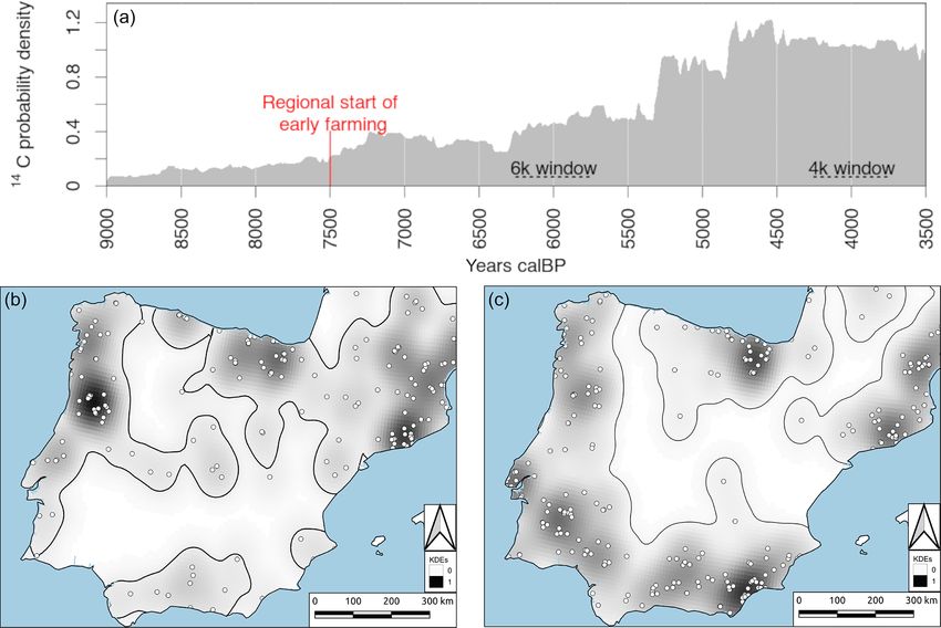
S. P. Harrison et al.: Development and testing scenarios for implementing land use and land cover changes 807
rent phase of the Palaeoclimate Modelling Intercomparison
Project (PMIP: Otto-Bleisner et al., 2017; Kageyama et al.,
2018). However, the datasets and protocol will also be useful
in later phases of other CMIP projects, including the Land
Use Model Intercomparison Project (LUMIP) and the Land
Surface, Snow and Soil Moisture Model Intercomparison
Project (LS3MIP) (Lawrence et al., 2016; van den Hurk et
al., 2016).
2 LandCover6k methodology
The primary source of information about human exploitation
of the landscape comes from archaeological data. In general,
these data are site specific, spatiotemporal coverage is often
patchy, and the types and quality of evidence available vary
between sites and regions. Generalizing from site-specific
data to landscape or regional scales involves making assump-
tions about human behaviour and cultural practices. Because
of the inherent uncertainties, we advocate an iterative ap-
proach to incorporate archaeological data into LULC sce-
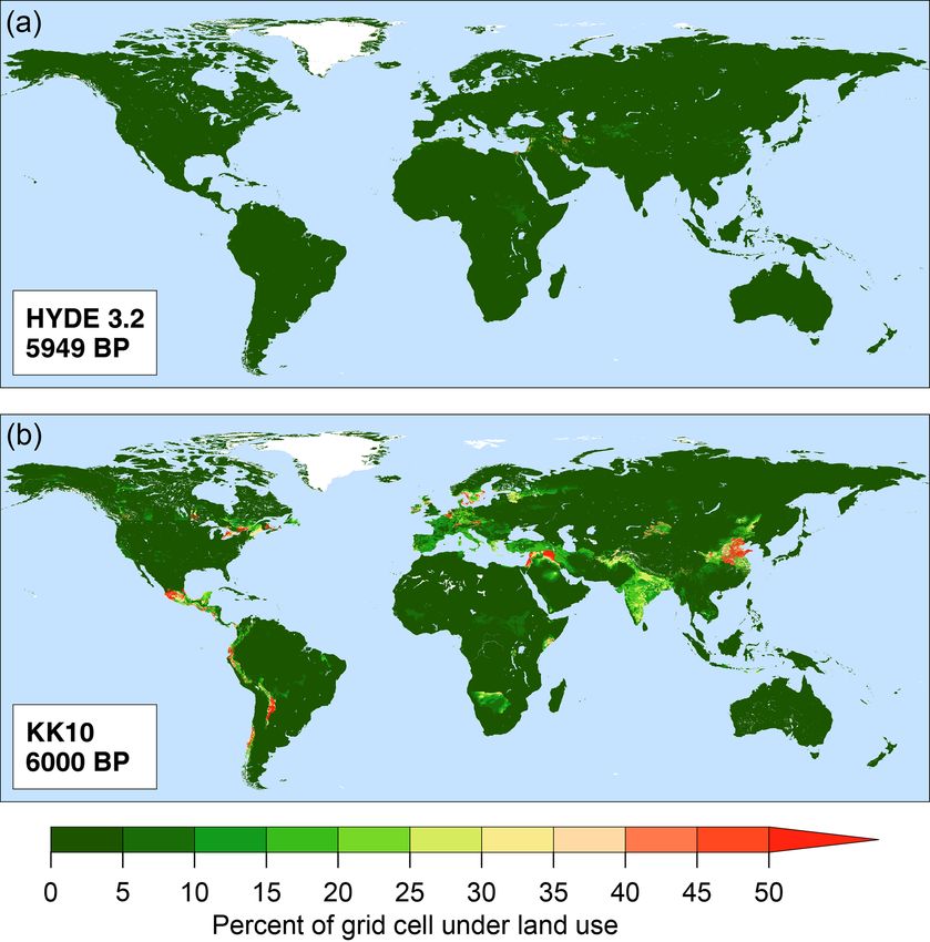
Figure 1. Land use at ca. 6000 years ago (6 ka BP, 4000 years BCE) narios in LandCover6k (Fig. 2). We propose revising the ex-
from the two widely used global historical land use scenarios isting LULC scenarios through the incorporation of diverse
HYDE 3.2 (a; Klein Goldewijk et al., 2017a) and KK10 (b; Kaplan archaeological inputs (Fig. 2, phase 1; see Sects. 3 and 4)
et al., 2011), illustrating the large disagreement between LULC sce- and testing the revised LULC scenarios for their plausibility
narios at a regional scale. In both scenarios, the land–sea mask and
and consistency with other lines of evidence (Fig. 2, phase 2
lake areas are for the present day.
with iterative testing; see Sects. 5–7). As a first test, the re-
vised LULC scenarios of the extent of cropland and grazing
land through time will be compared with independent data on
the development of LULC scenarios (Gaillard et al., 2018). land cover changes, specifically pollen-based reconstructions
LULC changes are taken into account in climate model of the extent of open land (see e.g. Trondman et al., 2015;
simulations currently being made in the current phase of the Kaplan et al., 2017) (Sect. 5). Further testing the LULC sce-
Coupled Model Intercomparison Project (CMIP6) for the narios involves sensitivity tests using global climate models
historic period and the future scenario runs (Eyring et al., (Sect. 6) and global carbon cycle models (Sect. 7). While
2016). They are also included in climate model simulations the computational cost of the climate model simulations can
of the past millennium (Jungclaus et al., 2017) in order to be minimized using equilibrium time-slice simulations, the
ensure that these runs mesh seamlessly with the historic carbon cycle constraint relies on transient simulations but
simulations. However, the Land Use Harmonization dataset may be derived from uncoupled, land-only simulations. Sim-
(LUH2: Hurtt et al., 2017) only extends back to 850 CE, ulated climates at key times can be evaluated against re-
and thus scenarios of LULC changes are currently not constructions of climate variables (e.g. Bartlein et al., 2011)
included in the CMIP6 palaeoclimate simulations, including (Sect. 6). The parallel evolution of CO2 and its isotopic com-
mid-Holocene simulations, that are used as a test of how position (δ 13 C) can be used to derive the carbon balance
well state-of-the-art climate models reproduce large climate of the terrestrial biosphere and the ocean separately (Elsig
changes. In this paper, we discuss how archaeological data et al., 2009); in combination with estimates for other con-
will be used to improve global LULC scenarios for the tributors to land carbon changes such as C sequestration by
Holocene. Given that there are large uncertainties associated peat build-up, it provides a strong constraint on the evolu-
with the primary data and further uncertainties may be tion of LULC through time. An underprediction or overpre-
introduced when this information is used to modify existing diction of anthropogenic LULC-related CO2 emissions dur-
LULC scenarios, we outline a series of tests that will be used ing a specific interval results in consequences for the dy-
to evaluate whether the revised LULC scenarios are consis- namics of the atmospheric greenhouse gas burden in subse-
tent with the changes implied by independent pollen-based quent times (Stocker et al., 2017) (Sect. 7). Thus, these tests
reconstructions of land cover and whether they produce more can be used to identify issues in the original archaeological
realistic estimates of both carbon cycle and climate changes. datasets and/or the way these data were incorporated into the
Finally, we present a protocol for implementing LULC in LULC scenarios that require further refinement. Phase 3 of
Earth system model simulations to be carried out in the cur- the project (Fig. 2) provides a protocol for the implementa-
www.geosci-model-dev.net/13/805/2020/ Geosci. Model Dev., 13, 805–824, 2020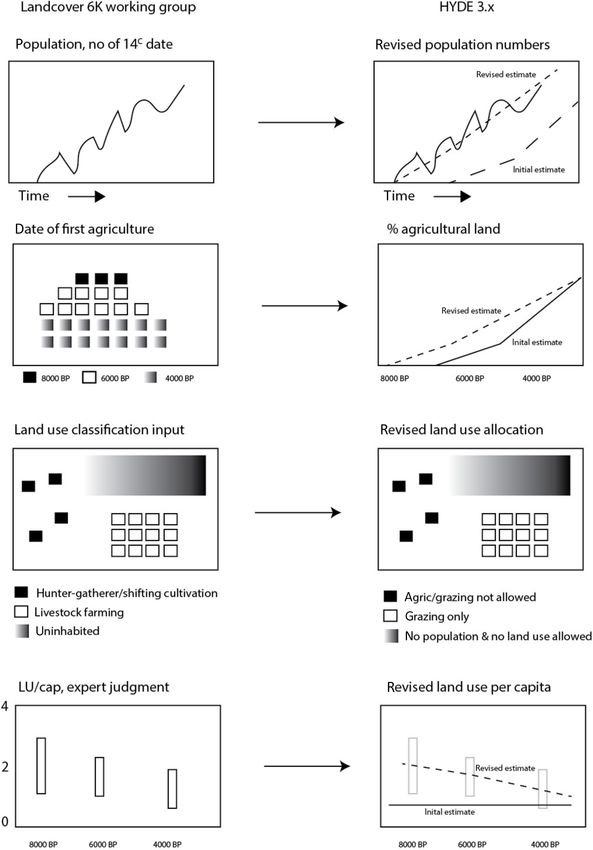
808           S. P. Harrison et al.: Development and testing scenarios for implementing land use and land cover changes

Figure 2. Proposed scheme for developing robust LULC scenarios through iterative testing and refinement as input to Earth system
model (ESM) simulations. The archaeological inputs developed in phase 1 can be used independently or together to improve the LULC
reconstructions; iterative testing of the LULC scenario reconstruction (phase 2) will ensure that these inputs are reliable before they are used
for ESM simulations (phase 3). The uppermost three LULC simulations capitalize on already planned baseline simulations without LULC;
the lowermost two simulations are envisaged as new sensitivity experiments.

tion of the revised LULC scenarios in Earth system model                  rectly reflected in the number of samples excavated and dated
simulations (Sect. 8).                                                    (Rick, 1987: Robinson et al., 2019). There are biases that
                                                                          could affect the expected one-to-one relationship between
                                                                          the number of people and the number of radiocarbon dates
3     Archaeological data inputs                                          on archaeological material, including lack of uniform sam-
                                                                          pling through time and space caused by different archaeo-
LandCover6k is creating a number of products that will be                 logical research interests and traditions in different regions
used to improve the LULC scenarios (Fig. 2). Here, we sum-                as well as increased preservation issues with increasing age,
marize the important features of these data products before               but these can be minimized by auditing the datasets. Assess-
showing how they will be incorporated within a scenario de-               ment of the robustness of population reconstructions through
velopment framework.                                                      time can be made statistically by comparing a null hypothe-
                                                                          sis of demographic growth constructed from an exponential
3.1    Population dynamics from 14 C data
                                                                          fit to the data with the actual record of the number of dates
                                                                          through time (Shennan et al., 2013; Timpson et al., 2014).
Radiocarbon is the most routinely used absolute dating tech-
                                                                          Mathematical simulations show that the method is relatively
nique in archaeology, especially for the Holocene. Many
                                                                          robust for large sample sizes (Williams, 2012). Radiocarbon
thousands of radiocarbon dates are available from the archae-
                                                                          dates have been successfully used in several regions to iden-
ological literature. A number of regional and pan-regional
                                                                          tify population fluctuations associated with hunter–gatherers
initiatives are compiling these records through exhaustive
                                                                          (Japan: Crema et al., 2016) and the introduction of farming
surveys of the archaeological literature (e.g. the Cana-
                                                                          and subsequent changes in farming regimes (western Europe:
dian Archaeological Radiocarbon Database: https://www.
                                                                          Shennan et al., 2013; Wyoming: Zahid et al., 2016; South Ko-
canadianarchaeology.ca/, last access: 14 February 2020).
                                                                          rea: Oh et al., 2017; see also Freeman et al., 2018) as well as
Statistical approaches, such as summed probability distribu-
                                                                          climatic oscillations (Ireland: Whitehouse et al., 2014).
tions (SPDs), can then be used to infer past demographic
fluctuations from these compilations (Fig. 3). This method
assumes that the more people there were, the more remains
of their various activities they left behind and that this is di-

Geosci. Model Dev., 13, 805–824, 2020                                                          www.geosci-model-dev.net/13/805/2020/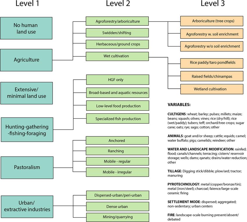
S. P. Harrison et al.: Development and testing scenarios for implementing land use and land cover changes                               809

Figure 3. Reconstruction of changes in population size on the Iberian Peninsula during the Holocene (9000 to 2000 BP, 9 ka to 2 ka BP)
using summed probability distributions (SPDs) of radiocarbon dates (a) (data after Balsera et al., 2015). The red line indicates the onset of
agriculture in the region. Panels (b) and (c) show areas under human use at 6 ka (b) and 4 ka (c) using kernel density estimates; the white
dots are actual archaeological sites, and the shading shows the implied density of occupation.

3.2   Date of first agriculture                                          areas where there is no (or only limited) evidence of land
                                                                         use and areas characterized by hunting, foraging, and fishing
Radiocarbon dates can also be used to track the timing and               activities, pastoralism, agriculture, and urban and/or extrac-
process of dispersal events, such as the diffusion of plant and          tive land use (Fig. 4). Except in the cases in which land use
animal domesticates from their initial centres of domestica-             is minimal (no human land use, extensive or minimal land
tion. Since the distribution of samples is often patchy, geosta-         use), further distinctions are subsequently made to encom-
tistical techniques such as kriging and splines are used to spa-         pass the diversity of land use activities in each land use type
tially interpolate the information in order to provide quantita-         (Fig. 4). A third level of distinction is made in the case of
tive estimates of the timing of spread. Work carried out in Eu-          two categories (agroforestry, wet cultivation) in which there
rope (Bocquet-Appel et al., 2009), Asia (Silva et al., 2015),            are very different levels of intervention in different regions.
and Africa (Russell et al., 2014) demonstrates that there are            Explanations of this terminology are given in Morrison et
different rates of diffusion even within a region, reflecting            al. (2018). The LandCover6k land use maps (see e.g. Fig. 5)
the possible impact of natural features (e.g. waterways, el-             will be based on different methods ranging from kernel den-
evation, ecology) on diffusion rates (Davison et al., 2006;              sity estimates to expert assessments depending on the quality
Silva and Steele, 2014). Numerous studies provide robust                 and quantity of the archaeological information available from
local estimates for the earliest regional occurrence of agri-            different regions.
culture, and these are being synthesized to provide a global                There is considerable variation in how intensely land is
product within LandCover6k (Fig. 2).                                     used both for crops and for grazing within broad land use
                                                                         categories both geographically and through time (Ford and
3.3   Global land use and livestock maps                                 Clarke, 2015; Styring et al., 2017). Maps of land use types
                                                                         do not provide direct information on the intensity of farm-
Maps of the distribution of archaeological sites or of areas
                                                                         ing practices or how they translate into per-capita land use.
linked to a given food production system have been produced
                                                                         Archaeological data about agricultural yields, combined with
for individual site catchments or small regions (e.g. Zimmer-
                                                                         information from analogous contemporary cultures, histori-
mann et al., 2009; Barton et al., 2010; Kay et al., 2019).
                                                                         cal information (e.g. Pongratz et al., 2008), and theoretical
LandCover6k is developing global land use maps for spe-
                                                                         estimates of land use required to meet dietary and energy re-
cific time windows using a global hierarchical classification
                                                                         quirements (e.g. Hughes et al., 2018), can be used to provide
of land use categories (Morrison et al., 2018) based on land
                                                                         regional estimates of per-capita land use for specific land use
use types that are widely recognized from the archaeological
                                                                         categories. LandCover6k will synthesize this information to
record. At the highest level, the maps distinguish between

www.geosci-model-dev.net/13/805/2020/                                                          Geosci. Model Dev., 13, 805–824, 2020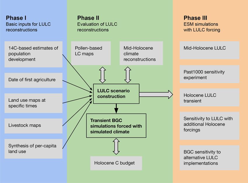
810           S. P. Harrison et al.: Development and testing scenarios for implementing land use and land cover changes

Figure 4. The hierarchical scheme of land use classes used for global mapping in LandCover6k (updated from Morrison et al., 2018).

allow regionally specific estimates of per-capita land use to         the level of detail will vary geographically, this information
be derived from the global land use maps.                             can be used to produce global livestock maps.
   Information about the extent of grazing land is an impor-             The harvesting of wood for domestic fires, building, and
tant input for the development of revised LULC scenarios              industrial activities such as transportation, pottery making,
but from a carbon cycle modelling perspective, the amount             and metallurgy is an important aspect of human exploita-
of biomass removed by grazing is also a key parameter.                tion of the landscape in the pre-industrial period (McGrath
Biomass loss varies not only with population size but also            et al., 2015). It has been argued that even Mesolithic hunter–
with the type of animal being reared (Herrero et al., 2013;           gatherer communities shaped their environment through
Phelps and Kaplan, 2017), and thus information about what             wood harvesting (Bishop et al., 2015). Approaches have been
animals were present at a given location and estimates of             developed to quantifying the wood harvest associated with
population sizes are needed for improving the existing LULC           archaeological settlements at specific times based on the evi-
scenarios. Although the conditions of bone preservation vary          dence of types of wood use, household energy requirements,
across the globe due to factors such as soil acidity, ani-            population size, and calorific value of the wood used (see
mal bones are routinely excavated (Lyman, 2008; Reitz and             e.g. Marston, 2009; Janssen et al., 2017). However, quantita-
Wing, 2008). Morphometric analyses of bones, along with               tive information on ancient technology and lifestyle is sparse,
collateral information such as age-related culling patterns,          and direct estimates of the amount of wood harvest through
make it possible to determine whether these are the remains           time are likely to remain highly uncertain (Marston et al.,
of domesticated species. We thus have a relatively precise            2017; Veal, 2017). Nevertheless, combining evidence-based
idea of when livestock were introduced into a region, what            inferential approaches with improved estimates of population
types of animals were being reared at a given time, and can           size should allow changes in wood harvesting to be taken into
also make informed estimates of population size. Although             account in constructing revised LULC scenarios.

Geosci. Model Dev., 13, 805–824, 2020                                                     www.geosci-model-dev.net/13/805/2020/
S. P. Harrison et al.: Development and testing scenarios for implementing land use and land cover changes 811
tural activity at a given time (e.g. either unsettled areas or ar-
eas occupied by hunter–gatherer communities) and provide
a further constraint on the geographic extent of the LULC
changes given by the scenarios (Fig. 6). The type of agricul-
ture, including whether the region was predominantly used
for tree or annual crops or for pasture, modifies the area of
open land specified in the LULC scenarios. Information on
the extent of rainfed versus irrigated agriculture, as indicated
by the presence of irrigation structures associated with ar-
chaeological sites, can also be used to refine the distribution
of these classes in the LULC scenarios. Per-capita land use
estimates and their changes through time (see e.g. Hughes et
al., 2018; Weiberg et al., 2019) provide a further refinement
of the LULC scenarios, allowing for a better characterization
of the distinction between e.g. areas given over to extensive
versus intensive animal production (rangeland versus pasture
in the HYDE 3.2 terminology). There will remain areas of the
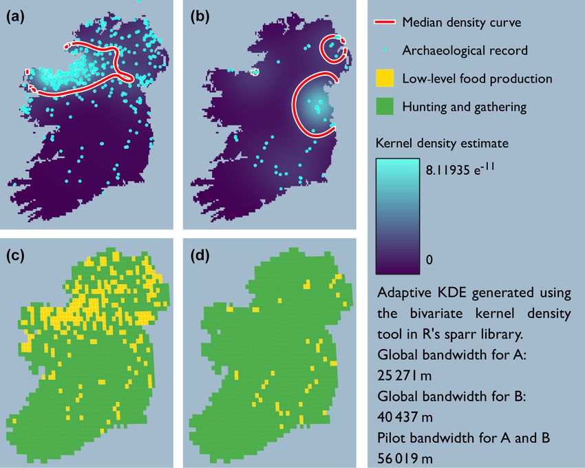
Figure 5. An example of regional land use mapping. (a, b) The world for which this kind of fine-grained information is not
distribution of known archaeological sites superimposed on ker- available. Nevertheless, by incorporating information when it
nel density estimates of the extent of land use based on the den-
exists, the LandCover6k products will contribute to a system-
sity of observations and (c, d) these data superimposed on the
LandCover6k land use classes for the middle Neolithic (3600–
atic refinement of existing LULC scenarios. Iterative testing
3400 years BCE, 5600–5400 years BP, 5.6–5.4 ka BP) (a, c) and of the revised scenarios will ensure that they are robust.
the early Neolithic (3750–3600 years BCE, 5750–5600 years BP,
5.7–5.6 ka BP) (b, d) in Ireland. Data points derive from 14 C-dated
archaeological sites and distributions of settlements and monuments 5 Using pollen-based reconstructions of land cover
that have been assigned to each archaeological period following the changes to evaluate LULC scenarios
dataset published in McLaughlin et al. (2016). The assigned land
use classes are inferred from archaeological material from one site Pollen-based vegetation reconstructions can be used to cor-
(or multiple sites) within the grid box. It should not be assumed that roborate archaeological information on the date of first
the whole grid cell was being used for agriculture during the mid- agriculture from the appearance of cereals and agricultural
dle and early Neolithic. Informed assessment suggests that agricul-
weeds. These reconstructions can also be used to test the
tural land (crop growing and grazing combined) probably occupied
10 %–15 % of the total grid area in the low-level food production
LULC reconstructions, either using relative changes in for-
regions of the eastern and western coastal areas, whilst agricultural est cover or reconstructions of the area occupied by dif-
land likely represents 5 % or less of the total grid cell area in inland ferent land cover types. LandCover6k uses the REVEALS
areas. pollen source-area model (Sugita, 2007) to estimate vegeta-
tion cover from fossil pollen assemblages. REVEALS pre-
dicts the relationship between pollen deposition in large lakes
4 Incorporation of archaeological data in LULC and the abundance of individual plant taxa in the surround-
scenarios ing vegetation at a large spatial scale (ca. 100 km × 100 km;
Hellman et al., 2008a, b) using models of pollen disper-
The existing LULC scenarios are substantially dependent on sal and deposition. REVEALS can also be used with pollen
historical regional population estimates at key times, which records from multiple small lakes or peat bogs (Trondman et
are then linearly interpolated to provide a year-by-year esti- al., 2016), although this results in larger uncertainties in the
mate of population. Estimates of regional population growth estimated area occupied by individual taxa. The estimates ob-
based on suitably screened 14 C data can be used to modify tained for individual taxa are summed to produce estimates
existing population growth curves (Fig. 6), both in terms of of the area occupied by either plant functional (e.g. summer-
establishing the initial date of human presence and by mod- green trees, evergreen trees) or land cover (e.g. open land,
ifying a linear growth curve to allow for intervals of popula- grazing land, cropland) types.
tion growth and decline. The geographic distribution of pollen records is uneven.
Information on the timing of the first appearance of agri- There are also many areas of the world where environments
culture at specific locations can be used to constrain the tem- that preserve pollen (i.e. lakes, bogs, forest hollows) are
poral record of LULC changes in the scenarios. This infor- sparse. Site-based reconstructions of land cover are there-
mation can also be used to allocate LULC changes geograph- fore interpolated statistically to produce spatially continu-
ically across regions (Fig. 6). Global land use maps can be ous reconstructions (Nielsen et al., 2012; Pirzamanbein et al.,
used to identify areas where there was no permanent agricul- 2014, 2018). LandCover6k uses a 1◦ resolution grid and all
www.geosci-model-dev.net/13/805/2020/ Geosci. Model Dev., 13, 805–824, 2020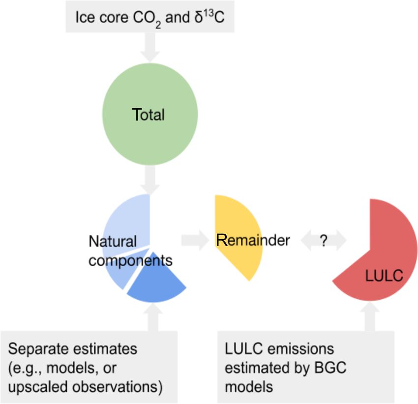
812           S. P. Harrison et al.: Development and testing scenarios for implementing land use and land cover changes

Figure 6. Schematic illustration of the proposed implementation of 14 C-based population estimates, date of first agriculture, land use maps,
and land use per-capita information in the HYDE model (here indicated as HYDE3.x). The archaeological data are represented as values
for a grid cell in geographic space at a given time for date of first agriculture and land use, but as a time series for a specific grid cell for
population and land use per capita. In the case of population estimates, date of first agriculture, and land use per-capita data, we show the
initial estimate and the revised estimate after taking the archaeological information into account in the HYDE3.x plot. It should be assumed
in the case of the land use mapping that the original estimate indicated no land use in this region.

available pollen records in each grid cell to produce an es-               reconstructions are partly expressed by their standard er-
timate of land cover per grid cell through time. The more                  rors (SEs). These SEs take into account the SE on the rel-
pollen records per grid cell and pollen counts per time win-               ative pollen productivity (RPP) of each plant taxon included
dow, the smaller the estimated error on the land cover recon-              in the REVEALS reconstructions and the variability between
struction. The uncertainties on the pollen-based REVEALS                   the site-specific REVEALS reconstructions (e.g. Trondman

Geosci. Model Dev., 13, 805–824, 2020                                                           www.geosci-model-dev.net/13/805/2020/
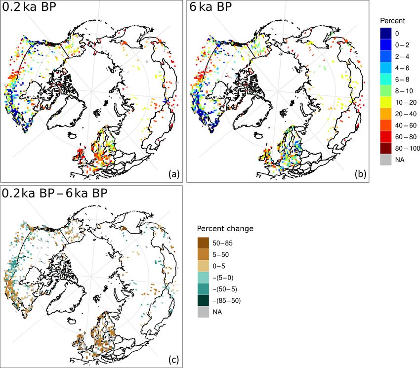
S. P. Harrison et al.: Development and testing scenarios for implementing land use and land cover changes                                813

Figure 7. Northern extratropical (> 40 ◦ N) mean fractional cover of open land at 6000 years ago (6 ka BP: b) and 200 years ago (0.2 ka BP: a)
estimated using REVEALS and the difference in fractional cover between the two periods (c). Red indicates an increase in open land and
blue a decrease (after Dawson et al., 2018).

et al., 2015). The uncertainties on the pollen-based land cover          tion of the REVEALS reconstructions is that RPP estimates
reconstructions are taken into account when these recon-                 are available for cultivated cereals but not for other culti-
structions are compared with LULC scenarios (Kaplan et al.,              vars or cropland weeds, so the LandCover6k pollen-based
2017).                                                                   reconstructions will generally underestimate cropland cover
   The REVEALS approach has already been used to pro-                    (Trondman et al., 2015). It may also be possible to use alter-
duce gridded reconstructions of changes in the amount of                 native pollen-based reconstructions of land cover changes,
open land through time across the northern extratropics                  such as the modern analogue approach (MAT: e.g. Tarasov et
(Fig. 7; Dawson et al., 2018) These reconstructions provide              al., 2007; Zanon et al., 2018), pseudo-biomization (e.g. Fyfe
mean plant cover for time slices of 500 years through the                et al., 2014), or STEPPS (Dawson et al., 2016). While none
Holocene until 0.7 ka BP and three historical time windows               of these methods require RPPs, MAT and STEPPS can only
(modern – 0.1, 0.1–0.35, and 0.35–0.7 ka BP). The more                   be applied in regions where the pollen datasets have dense
pollen samples per time interval and pollen records per grid             coverage (such as Europe and North America), and pseudo-
cell, the more years within the 500-year time slice will be              biomization is affected by the non-linearity of the pollen–
represented in the reconstruction. This implies that the num-            vegetation relationship that the REVEALS approach is de-
ber of years represented in a time-slice reconstruction varies           signed to remove.
in space and time.                                                          Comparison of the reconstructions of the extent of open
   A major limitation in applying REVEALS globally is the                land with the LULC deforestation scenarios will provide a
requirement for information about the relative pollen pro-               first evaluation of the realism of the revised LULC scenar-
ductivity (RPP) of individual pollen taxa, which is currently            ios (e.g. Kaplan et al., 2017). Underestimation or overesti-
largely lacking for the tropics. However, LandCover6k has                mation of open land in the LULC scenarios is not neces-
been collecting RPPs for China, south-east India, Cameroon,              sarily an indication that these scenarios are inaccurate be-
Brazil, and Argentina, and pollen-based land cover recon-                cause (a) pollen-based reconstructions cannot distinguish
structions will be available for sufficient parts of the tropics         between anthropogenic and climatically determined natural
to allow the testing of the LULC scenarios. Another limita-              open land (e.g. natural grasslands, steppes, wetlands), and

www.geosci-model-dev.net/13/805/2020/                                                           Geosci. Model Dev., 13, 805–824, 2020
814 S. P. Harrison et al.: Development and testing scenarios for implementing land use and land cover changes
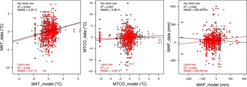
Figure 8. Quantitative comparison of the change in climate between the mid-Holocene (6 ka) and the pre-industrial period as shown by
pollen-based reconstructions gridded to 2 × 2◦ resolution to be compatible with the model resolution (from Bartlein et al., 2011) and in
simulations with and without the incorporation of land use change (from Smith et al., 2016). This figure illustrates the approach that will be
taken to evaluate the impact of new LULC scenarios on climate. The imposed land use changes at 6000 years ago (6 ka BP) were derived from
the KK10 scenario (Kaplan et al., 2011). The plots show comparisons of mean annual temperature (MAT), mean temperature of the coldest
month (MTCO), and mean annual precipitation (MAP) for the northern extratropics (north of 30◦ N); each dot represents a model grid cell in
which comparisons with the pollen-based reconstructions are possible. Although the incorporation of land use produces somewhat warmer
and wetter climates in these simulations, overall the incorporation of land use produces no improvement of the simulated climates at sites
with pollen-based reconstructions.
(b) REVEALS underestimates cropland cover because there in central Eurasia (Mauri et al., 2014; Harrison et al., 2015;
are no RPP estimates for cultivars other than cereals. How- Bartlein et al., 2017). There are discernible anthropogenic
ever, overestimation of the area of open land in the LULC impacts on the landscape in many of these regions by 6 ka, al-
scenarios might suggest problems either in the archaeologi- though they are not as strong as during the later Holocene and
cal inputs or their implementation, especially for times or re- they are not present everywhere. Nevertheless, the 6 ka BP
gions for which other evidence indicates cereals were the ma- interval provides a good focus for testing whether improve-
jor crop. In this sense, despite potential problems, the Land- ments to the LULC scenarios produces more realistic simu-
Cover6k pollen-based reconstructions of land cover will pro- lations of climate. Such an evaluation would need to go be-
vide an important independent test of the revised LULC sce- yond the global comparison made here (Fig. 8) to regional
narios. comparisons to identify whether improvements in simulated
climate in regions where there is a large anthropogenic im-
pact on land cover result in a degradation in the simulated
6 Testing the reliability of improved scenarios using climate elsewhere.
climate model simulations
A second test of the realism of the improved LULC scenar- 7 Testing the reliability of improved scenarios using
ios is to examine whether incorporating LULC changes im- carbon cycle models
proves the realism of the simulated climate when compared
to palaeoclimate reconstructions (Fig. 8). The mid-Holocene Carbon cycle modelling will be used as a further test of the
(6000 years ago, 6 ka BP) is an ideal candidate for such a realism of the improved LULC scenarios. Two constraints
test because benchmark datasets of quantitative climate re- are available for testing the realism of past LULC scenar-
constructions are available (e.g. Bartlein et al., 2011), the ios. First, reconstructions of LULC history must converge on
interval has been a focus through multiple phases of PMIP, the present-day state, which is relatively well constrained by
control simulations with no LULC have already been run, satellite land cover observations and national statistics on the
and evaluation of these simulations has identified regions amount of land under use. Reconstructing the extent of past
where there are major discrepancies between simulated and LULC change thus reduces to allocating a fixed total amount
reconstructed climates e.g. the observed expansion of North- of land conversion from natural to agricultural use over time.
ern Hemisphere monsoons, climate changes over Europe, the More conversion in earlier periods implies less conversion
magnitude of high-latitude warming, and wetter conditions in later periods. At the continental to global scale, cumu-
Geosci. Model Dev., 13, 805–824, 2020 www.geosci-model-dev.net/13/805/2020/S. P. Harrison et al.: Development and testing scenarios for implementing land use and land cover changes 815
lative LULC emissions scale linearly with the agricultural
area. LULC scenarios that converge to the present-day state
also converge to within a small range of cumulative histori-
cal emissions (Stocker et al., 2011, 2017). Deviations from a
linear relationship between extent and emissions are due to
differences in biomass density in potential natural and agri-
cultural vegetation of different regions affected by anthro-
pogenic LULC. Differences in cumulative emissions for al-
ternative LULC reconstructions with an identical present-day
state are due to the long response time of soil carbon con-
tent following a change in carbon inputs and soil cultivation.
Conserving the total extent of LULC (and allocating a fixed
total expansion over time) is thus approximately equivalent
to conserving cumulative historical LULC emissions. Thus,
more LULC CO2 emissions in earlier periods imply less CO2
emissions in more recent periods.
The total C budget of the terrestrial biosphere provides a
second constraint on LULC emissions through time. The net Figure 9. Illustration of the terrestrial C budget approach to eval-
C balance of the land biosphere, which reflects the sum of uate LULC. The total terrestrial C balance (green circle, “total”)
all natural and anthropogenic effects on terrestrial C storage, is constrained by ice core records of CO2 and its isotopic signa-
can be reconstructed from ice core data of past CO2 concen- ture (δ 13 C). Estimates for C balance changes in different natural
trations and δ 13 C composition (Elsig et al., 2009). Provided land carbon cycle components (e.g. peatlands, permafrost, forest
expansion or retreat, desert greening) are estimated independently
that all of the natural contributions to the land C inventory
(blue slices, “natural components”) either from empirical upscal-
(e.g. the build-up of natural peatlands: Loisel et al., 2014) can
ing of site-scale observations or from model-based analyses (car-
be specified from independent evidence, the anthropogenic bon cycle models forced with varying climate). The remainder (yel-
sources can be estimated as the difference between the total low slice, “remainder”) is then calculated as the total terrestrial
terrestrial C budget and natural contributions (Fig. 9) at any C balance (green circle, “total”) minus the sum of the separate
specific time. estimates of the natural components (blue slices, “natural compo-
Transient simulations with a model that simulates CO2 nents”). The remainder is effectively the emissions resulting from
emissions in response to anthropogenic LULC can be used to LULC changes and can therefore be compared to LULC CO2 emis-
test the reliability of the LULC scenarios by comparing re- sion estimates by carbon cycle models.
sults obtained with prescribed LULC changes through time
against a baseline simulation without imposed LULC. This
will necessitate making informed decisions about the frac- 8 Implementation of LULC in Earth system model
tion of land under cultivation that is abandoned or left fallow simulations
each year and the maximum extent of land affected by such
episodic cultivation. We envisage using several different of- We propose a series of simulations to examine the impact of
fline carbon cycle models for this purpose in order to take LULC using the revised LULC scenarios from LandCover6k
account of uncertainties associated with differences between and building on climate model experiments that are currently
the carbon cycle models. The carbon cycle simulations will being run either in CMIP6-PMIP4 (midHolocene, past1000)
be driven by climate outputs (temperature, precipitation, and or within PMIP although not formally included as CMIP6-
cloud cover) from an existing transient climate simulation PMIP4 experiments.
made with the ECHAM model (Fischer and Jungclaus, 2011) The midHolocene (and its corresponding piControl) simu-
and CO2 prescribed from ice core records. The CO2 emis- lation is one of the PMIP entry cards in the CMIP6-PMIP4
sion estimates from these two simulations will then be eval- experiments (Kageyama et al., 2018; Otto-Bliesner et al.,
uated using C budget constraints. This evaluation will allow 2017), and it is therefore logical to propose this period
us to pinpoint potential discrepancies between known terres- for LULC simulations. The LULC sensitivity experiment
trial C balance changes and estimated LULC CO2 emissions (midHoloceneLULC) should therefore follow the CMIP6-
in given periods over the Holocene. PMIP4 protocol; that is, it should be run with the same
climate model components and following the same proto-
cols for implementing external forcings as used in the two
CMIP6-PMIP4 experiments (Table 1). Thus, if the piControl
and midHolocene simulations are run with interactive (dy-
namic) vegetation, then the midHoloceneLULC experiment
should also be run with dynamic vegetation in regions where
www.geosci-model-dev.net/13/805/2020/ Geosci. Model Dev., 13, 805–824, 2020816 S. P. Harrison et al.: Development and testing scenarios for implementing land use and land cover changes
Table 1. Boundary conditions for CMIP6-PMIP4 and the mid-Holocene LULC experiments. The boundary conditions for the CMIP6-PMIP4
piControl and midHolocene are described in Otto-Bleisner et al. (2017) and are given here for completeness.
Boundary conditions 1850 CE 6 ka 6 ka LULC
(DECK (midHolocene) (midHoloceneLULC)
piControl)
Orbital Eccentricity 0.016764 0.018682 0.018682
parameters Obliquity 23.459 24.105 24.105
Perihelion – 180 100.33 0.87 0.87
Vernal equinox Noon, 21 March Noon, 21 March Noon, 21 March
Greenhouse Carbon dioxide (ppm) 284.3 264.4 264.4
gases Methane (ppb) 808.2 597.0 597.0
Nitrous oxide (ppb) 273.0 262.0 262.0
Other GHGs DECK piControl 0 0
Other Solar constant TSI: 1360.747 As piControl As piControl
boundary Palaeogeography Modern As piControl As piControl
conditions Ice sheets Modern As piControl As piControl
Vegetation Interactive Interactive Pasture and crop;
distribution prescribed
from a revised scenario
DECK piControl As piControl Pasture and crop;
distribution prescribed
from a revised scenario
Aerosols interactive Interactive Interactive
DECK piControl As piControl As piControl
there is no LULC change. For most models, this means that the LandCover6k scenario, the specifications of other forc-
the LULC forcing is imposed as a fraction of the grid cell ings would then follow the recommendations for the CMIP6-
and the remaining fraction of the grid cell has simulated nat- PMIP4 past1000 simulation.
ural vegetation. These new mid-Holocene simulations would A transient climate simulation for a longer period of the
allow for a better understanding of the relationship between Holocene would provide a more stringent test of the impact
climate changes and land–surface feedbacks (including snow of LULC on the coupled Earth system. We suggest that this
albedo feedbacks), as well as the role of water recycling at transient simulation (holotrans) should start from the pre-
a regional scale. Thus, modelling groups who are running existing midHolocene simulation to capitalize on the fact that
the midHolocene experiment with a fully interactive carbon the midHolocene simulation has been spun up sufficiently
cycle could also run the LULC experiment allowing atmo- long (Otto-Bleisner et al., 2017) to ensure that the ocean and
spheric CO2 to evolve interactively, subject to the simulated land carbon cycle is in equilibrium at the start of the tran-
ocean and land C balance. sient experiment (Table 2). In order to be consistent with
The real strength of the revised LULC scenarios is to pro- the CMIP6-PMIP4 midHolocene protocol (Otto-Bleisner et
vide boundary conditions for transient climate model sim- al., 2017), changes in orbital forcing should be specified
ulations. The CMIP6-PMIP4 simulation of 850–1850 CE from Berger and Loutre (1991), and year-by-year changes
(past1000) already incorporates LULC changes as a forcing in CO2 , CH4 , and N2 O should be specified following Joos
(Jungclaus et al., 2017) based on a harmonized dataset that and Spahni (2008). LULC changes should be implemented
provides LULC changes from 850 through 2015 CE (Hurtt et by imposing crop and pasture area through time as speci-
al., 2017), which in turn draws on output from the HYDE3.2 fied in the revised LULC scenarios; elsewhere, the simulated
scenario (Klein Goldewijk et al., 2017a). The past1000 pro- vegetation should be active. It will be necessary to run the
tocol (Jungclaus et al., 2017) acknowledges that this default Holocene transient climate simulation in two steps. A first
land use dataset is at the lower end of the spread in estimates simulation (holotrans_LULC) should be run using prescribed
of early agricultural area indicated by other LULC scenar- atmospheric CO2 concentration, even though the carbon cy-
ios and recommends that modelling groups run additional cle is fully interactive, because this will establish the consis-
sensitivity experiments using alternative maximum and min- tency of the carbon cycle in the land surface model. However,
imum scenarios. The revised LULC scenarios created by once this is done it will be possible to rerun the simulations
LandCover6k could be used as an alternative to these maxi- with interactive CO2 emissions. Table 3 provides a summary
mum and minimum scenarios. Other than the substitution of of the proposed ESM simulations.
Geosci. Model Dev., 13, 805–824, 2020 www.geosci-model-dev.net/13/805/2020/S. P. Harrison et al.: Development and testing scenarios for implementing land use and land cover changes 817
Table 2. Boundary conditions for baseline PMIP Holocene transient (6 ka BP to 1850 CE) and LULC transient simulations.
Mode Source or value LULC experiment
Orbital parameters Transient As baseline simulation
Greenhouse gases CO2 Transient Dome C As baseline simulation
CH4 Combined EPICA & GISP record As baseline simulation
N2 O Combined EPICA NGRIP, & TALDICE record As baseline simulation
Solar forcing Transient Steinhilber et al. (2012) As baseline simulation
Volcanic forcing Transient To be determined As baseline simulation
Palaeogeography Constant at PI values Modern As baseline simulation
Ice sheets Constant at PI values Modern As baseline simulation
Vegetation Interactive LC6k transient pasture and
crop distribution imposed
Aerosols Constant at PI values As baseline simulation
Table 3. Summary of proposed simulations.
Name Mode Purpose
piControl Equilibrium Standard CMIP6-PMIP4 simulation
midHolocene Equilibrium Standard CMIP6-PMIP4 simulation
midHoloceneLULC Equilibrium Sensitivity to LULC changes
holotrans Transient Baseline fully transient simulation from
6 ka onwards, with no LULC
holotrans_LULC Transient Fully transient simulation from 6 ka
onwards, with LULC imposed
Unlike the situation for the mid-Holocene, wherein there sensitivity tests could be run to take these additional forcings
is a global climate benchmark dataset (Bartlein et al., 2011) into account. In the case of solar and volcanic forcing, this
which provides reconstructions of multiple bioclimatic vari- would also ensure that the transient holotrans simulations
ables of seasonal temperature and moisture, the opportunities mesh seamlessly with the past1000 simulation. Changes in
for quantitative evaluation of the holotrans simulated climate solar variability during the Holocene should be specified
are more limited. Seasonal temperature reconstructions are from Steinhilber et al. (2012). There are records of volcanic
available for Europe (Davis et al., 2003) and North America forcing for the past 2000 years (Sigl et al., 2015; Toohey
(Viau et al., 2006; Viau and Gajewski, 2009). Although there and Sigl, 2017), and these are used in the past1000 sim-
is a new global dataset that provides global temperature re- ulation. Observationally constrained estimates of volcanic
constructions for the Holocene (Kaufman et al., 2020), it is stratospheric aerosol for the Holocene are currently under
based on only 472 terrestrial records worldwide, and the re- development (Michael Sigl, personal communication, 2019)
sults for zonally averaged temperature changes are therefore and could be implemented as an additional sensitivity exper-
likely to be more robust than the regional details. There are iment when available. Changes in atmospheric dust loading
also time series reconstructions for individual sites outside are not included in the past1000 simulation but are important
these two regions (e.g. Nakagawa et al., 2002; Wilmshurst et during the earlier part of the Holocene (Pausata et al., 2016;
al., 2007; Ortega-Rosas et al., 2008). Furthermore, the simu- Tierney et al., 2017; Messori et al., 2019). Although continu-
lated time course of CO2 emissions can be compared to the ous reconstructions of dust loading through the Holocene are
ice core records. not available, it would be possible to use estimates for partic-
The CMIP6-PMIP4 midHolocene simulations are stylized ular time slices (Egerer et al., 2018) to test the sensitivity to
experiments lacking several potential forcings (in addition to this forcing.
LULC), including changes in atmospheric dust loading, solar
irradiance, and volcanic forcing. We suggest that additional
www.geosci-model-dev.net/13/805/2020/ Geosci. Model Dev., 13, 805–824, 2020818 S. P. Harrison et al.: Development and testing scenarios for implementing land use and land cover changes
9 Outcomes and perspectives accounted for (Shevliakova et al., 2009). It would therefore
be interesting to run additional simulations accounting for
LandCover6k has developed a scheme for using archaeo- net land use change and indeed separating out the effects of
logical information to improve existing scenarios of LULC wood harvesting and shifting cultivation.
changes during the Holocene, specifically by using archae- We anticipate that it will be possible to incorporate re-
ological data to provide better estimates of regional popu- alistic LULC scenarios for the mid-Holocene as part of
lation changes through time, better information on the date the climate model sensitivity experiments planned during
of the initiation of agriculture in a region, more regionally PMIP4. Such experiments will complement the CMIP6-
specific information about the type of land use, and more nu- PMIP4 baseline model experiments by providing insights
anced information about land use per capita than currently into whether discrepancies between simulated and observed
implemented in the LULC scenarios generated by HYDE and 6 ka climate could be the result of incorrect specification of
KK10. While the final global datasets are still in production, the land–surface boundary conditions. However, the incor-
fast-track priority products have been created and their im- poration of archaeological information into LULC scenarios
pact on current scenarios is being tested. clearly makes it possible to target other interesting periods
Although the work of LandCover6k will provide more for such experiments, for example to explore whether land
solid knowledge about anthropogenic modification of the use changes played a role in abrupt events such as the 4.2 ka
landscape, some information will inevitably be missing and event, the impact of population declines in the Americas as a
some key regions will be poorly covered. There will still be consequence of European colonization (1500–1750 CE), or
large uncertainties associated with revised LULC scenarios, the changes in land use globally during the industrial era
even though these will be based on more solid evidence than (post-1850 CE).
the existing LULC scenarios. Documenting the uncertainties In addition to providing a protocol for the PMIP 6 ka sen-
in the archaeological inputs and their impacts on the revised sitivity experiments, we have devised a protocol for imple-
scenarios is an important goal of the LandCover6k project. menting the optimal LULC reconstructions for the Holocene
We propose using the information about the uncertainties in in transient climate model or ESM experiments. The goal
the archaeological data sources to generate multiple LULC here is to provide one of the necessary forcings that could be
scenarios comparable to the “low-end” and “high-end” sce- used for transient simulations in future phases of PMIP. This
narios used for e.g. future projections. Furthermore, we have will allow for an assessment of LULC in these simulations
proposed a series of tests that will help to evaluate the realism and therefore help address issues that are a focus for other
of the final scenarios based on independent evidence from MIPs e.g. LUMIP or LS3MIP. When these new forcings are
pollen-based reconstructions of land cover, reconstructions created, they will be made available through the PMIP4 web-
of climate, and carbon cycle constraints. These tests should site (https://pmip4.lsce.ipsl.fr/doku.php/exp_design:lgm, last
help in identifying which of the potential LULC reconstruc- access: 14 February 2020, PMIP4 repository, 2017) and the
tions are most realistic and in constraining the sources of un- Earth System Grid Federation (ESGF) Input4MIPS reposi-
certainty. tory (https://esgf-node.llnl.gov/projects/input4mips/, last ac-
We have proposed the use of offline carbon cycle simu- cess: 14 February 2020, with details provided in the “in-
lations solely as a test of the realism of the revised LULC put4MIPs summary” link). Modelling groups who run either
scenarios. Quantifying the LULC contribution to CO2 emis- equilibrium or transient climate model experiments follow-
sions during the Holocene would require additional simula- ing this protocol are encouraged to follow the standard CMIP
tions in which other forcings (climate, atmospheric CO2 , in- protocol for archiving their simulations through the ESGF.
solation) are kept constant. The difference in simulated total
terrestrial C storage between these simulations and LULC
simulations provides an estimate of primary emissions (Pon- Code and data availability. The data used for Fig. 1 are
gratz et al., 2014) and avoids additional model uncertainty publicly available. The HYDE3.2 data can be downloaded
regarding the sensitivity of land C storage to atmospheric from: https://doi.org/10.17026/dans-25g-gez3 (Klein Gold-
CO2 or climate being included in emission estimates. There ewijk, 2017). The KK10 data can be downloaded from:
https://doi.org/10.1594/PANGAEA.871369 (Kaplan and
are other sensitivity tests that would be useful. For exam-
Krumhardt, 2011). The code and data used to generate Fig. 1 are
ple, vegetation–carbon cycle models differ in their ability to available from: https://github.com/jedokaplan/ALCC_comparison_
account for gross land use transitions within grid cells (Ar- figure (Kaplan, 2020). The data and code used to generate Fig. 3 are
neth et al., 2017). This is critical for simulating the effects of available from: https://github.com/mavdlind/GMD (Vander Linden,
non-permanent agriculture, whereby land is simultaneously 2020). The data and code used to generate Fig. 5 are available from:
abandoned and reclaimed within the extent of a model grid https://doi.org/10.5281/zenodo.3625226 (Lewin and Whitehouse,
cell. Such shifting cultivation-type agriculture implies for- 2020. The European pollen-based reconstructions used in Fig. 7 are
est degradation in areas recovering from previous land use available at: https://doi.org/10.1594/PANGAEA.897303 (Gaillard,
and leads to substantially higher LULC emissions compared 2019). The pollen data used to generate the Siberian reconstructions
to model estimates wherein only net land use changes are are available from: https://doi.org/10.1594/PANGAEA.898616.
Geosci. Model Dev., 13, 805–824, 2020 www.geosci-model-dev.net/13/805/2020/You can also read