Spatio-temporal variations in lateral and atmospheric carbon fluxes from the Danube Delta
←
→
Page content transcription
If your browser does not render page correctly, please read the page content below
Biogeosciences, 18, 1417–1437, 2021
https://doi.org/10.5194/bg-18-1417-2021
© Author(s) 2021. This work is distributed under
the Creative Commons Attribution 4.0 License.

Spatio-temporal variations in lateral and atmospheric carbon fluxes
from the Danube Delta
Marie-Sophie Maier1,2 , Cristian R. Teodoru1 , and Bernhard Wehrli1,2
1 Institute of Biogeochemistry and Pollutant Dynamics, ETH Zürich, Zurich 8092, Switzerland
2 Eawag,   Swiss Federal Institute of Aquatic Science and Technology, Kastanienbaum 6047, Switzerland

Correspondence: Marie-Sophie Maier (marie-sophie.maier@usys.ethz.ch)

Received: 28 May 2020 – Discussion started: 8 July 2020
Revised: 26 November 2020 – Accepted: 10 December 2020 – Published: 24 February 2021

Abstract. River deltas, with their mosaic of ponds, channels      portionately to the delta’s emissions, considering their lim-
and seasonally inundated areas, act as the last continental hot   ited surface area. In terms of lateral export, we estimate
spots of carbon turnover along the land–ocean aquatic con-        the net total export (the sum of dissolved inorganic car-
tinuum. There is increasing evidence for the important role       bon, DIC, dissolved organic carbon, DOC, and particulate
of riparian wetlands in the transformation and emission of        organic carbon, POC) from the Danube Delta to the Black
terrestrial carbon to the atmosphere. The considerable spatial    Sea to be about 160 ± 280 GgC yr−1 , which only marginally
heterogeneity of river deltas, however, forms a major obsta-      increases the carbon load from the upstream river catch-
cle for quantifying carbon emissions and their seasonality.       ment (8490 ± 240 GgC yr−1 ) by about 2 %. While this con-
The water chemistry in the river reaches is defined by the up-    tribution from the delta seems small, deltaic carbon yield
stream catchment, whereas delta lakes and channels are dom-       (45.6 gC m−2 yr−1 ; net export load/surface area) is about 4
inated by local processes such as aquatic primary production,     times higher than the riverine carbon yield from the catch-
respiration or lateral exchange with the wetlands. In order to    ment (10.6 gC m−2 yr−1 ).
quantify carbon turnover and emissions in the complex mo-
saic of the Danube Delta, we conducted monthly field cam-
paigns over 2 years at 19 sites spanning river reaches, chan-
nels and lakes. Here we report on the greenhouse gas fluxes       1   Introduction
(CO2 and CH4 ) from the freshwater systems of the Danube
Delta and present the first seasonally resolved estimates of      In an attempt to improve global climate models, the role of
its freshwater carbon emissions to the atmosphere. Further-       rivers and their deltas and estuaries in the carbon cycle has
more, we quantify the lateral carbon transport of the Danube      received increased attention for more than a decade (IPCC,
River to the Black Sea.                                           2007). Back then, the perception shifted from rivers as be-
   We estimate the delta’s CO2 and CH4 emissions to be            ing mere lateral conduits of particulate and dissolved carbon
65 GgC yr−1 (30–120 GgC yr−1 , a range calculated using 25        species to a so-called active pipe concept, where rivers are
to 75 percentiles of observed fluxes), of which about 8 % are     considered as being efficient biogeochemical reactors with
released as CH4 . The median CO2 fluxes from river branches,      the potential to release significant amounts of carbon as CO2
channels and lakes are 25, 93 and 5.8 mmol m−2 d−1 , re-          and CH4 directly to the atmosphere (Cole et al., 2007; IPCC,
spectively. Median total CH4 fluxes amount to 0.42, 2.0 and       2013). A multitude of global upscaling studies (e.g. Tranvik
1.5 mmol m−2 d−1 . While lakes do have the potential to act       et al., 2009; Regnier et al., 2013; Raymond et al., 2013) es-
as CO2 sinks in summer, they are generally the largest emit-      timated the riverine and lacustrine fluxes of CO2 and CH4
ters of CH4 . Small channels showed the largest range in          to the atmosphere on a persistently fragmentary database,
emissions, including a CO2 and CH4 hot spot sustained by          considering spatial and temporal coverage – especially of
adjacent wetlands. Thereby, the channels contribute dispro-       headwater streams and large lowland rivers (Hartmann et al.,
                                                                  2019; Drake et al., 2018).

Published by Copernicus Publications on behalf of the European Geosciences Union.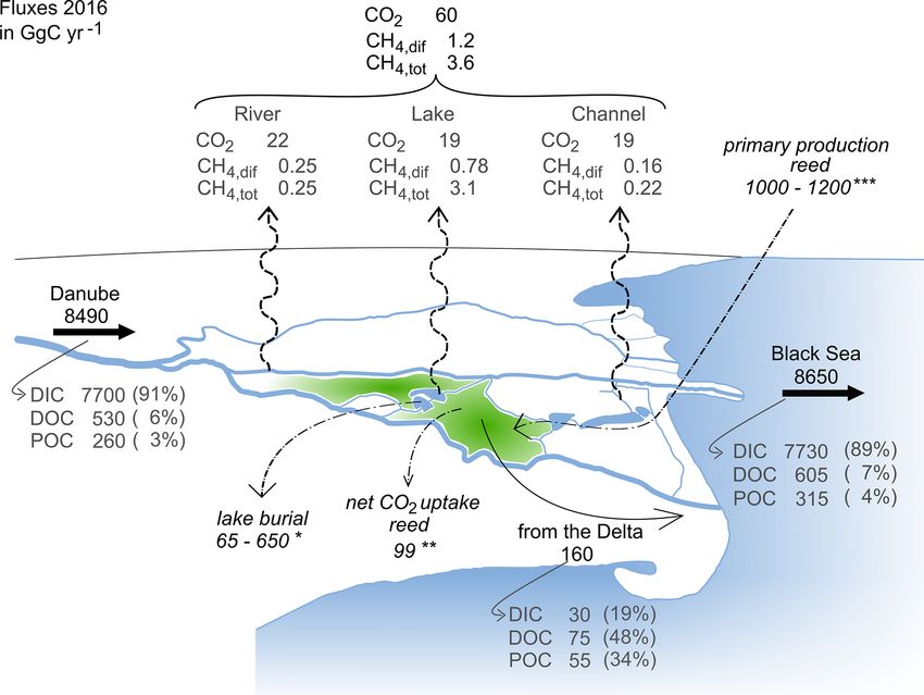
1418                              M.-S. Maier et al.: Spatio-temporal variations in lateral and atmospheric carbon fluxes

   Along the land–ocean aquatic continuum, about 0.9–             ject to CO2 and CH4 evasion studies (Sawakuchi et al.,
0.95 PgC yr−1 are estimated to be transferred laterally by        2014; Dubois et al., 2010; Teodoru et al., 2015), others,
rivers to the ocean (Regnier et al., 2013; Kirschbaum et al.,     such as the Nile and Danube, remained unchartered terri-
2019). Half of the carbon exported to the ocean is in the         tory in that respect. Both the Nile and Danube rivers rep-
form of dissolved inorganic carbon (DIC), while the other         resent one end of the river delta spectrum since they show
half consists of particulate and dissolved organic carbon         little exposure to tidal action. Therefore, these deltas ex-
(POC and DOC, respectively) in about equal shares (Li et          perience seasonal flooding, instead of (semi-)diurnal flood-
al., 2017; Kirschbaum et al., 2019). Recent estimates sug-        ing determined by tidal action. Flooding can, in addition to
gest that about 50 % to > 70 % of the carbon inputs from          groundwater drainage and surface runoff, transport substan-
terrestrial ecosystems degas as CO2 and CH4 along the way         tial amounts of terrestrial carbon to aquatic systems (Abril
to the ocean (Drake et al., 2018; Stumm and Morgan, 1981;         and Borges, 2019). We thus anticipate seasonal variability in
Kirschbaum et al., 2019; Cole et al., 2007), making this the      CO2 and CH4 emissions and in lateral carbon transport from
most important export flux of terrestrial carbon from inland      the Danube Delta to the ocean.
waters. While rivers could emit 0.65–1.8 PgC yr−1 (Lauer-             In this study, we estimate delta-scale atmospheric CO2
wald et al., 2015; Raymond et al., 2013), lakes and reser-        and CH4 emissions for the Danube Delta and the lateral car-
voirs could add another 0.3–0.58 PgC yr−1 (Raymond et al.,        bon transport of the Danube River to the Black Sea. We hy-
2013; Holgerson and Raymond, 2016). Earlier works on in-          pothesized that the hydromorphology of the different water-
ner estuaries, salt marshes and mangroves estimate their con-     scapes would influence the outgassing behaviour of green-
tribution to be another 0.39–0.52 PgC yr−1 (Borges, 2005;         house gases by governing gas exchange and biogeochemi-
Borges et al., 2005). So, river deltas and estuaries seem to      cal processes. The resulting differences in atmospheric fluxes
contribute almost equally to CO2 and CH4 emissions as lakes       would require treating the waterscapes separately in the up-
and reservoirs, despite representing only about one-sixth of      scaling process. Furthermore, we anticipated that the sea-
their global surface area (Cai et al., 2013; Holgerson and        sonality of the flooding affects both atmospheric and lateral
Raymond, 2016).                                                   fluxes.
   Deltas and estuaries represent hot spots of carbon turnover        To capture this spatial and temporal variability, we con-
and CO2 and CH4 emissions due to the high nutrient load,          ducted a systematic study covering 19 sites in the Danube
large productivity and seasonal flooding. However, differ-        Delta over 2 years, with monthly sampling intervals. Based
ences in geomorphology, anthropogenic alterations, complex        on this time series, we address the systematic differences be-
hydrology and the influence of tides are just a few of the        tween the delta’s main waterscapes (river branches, chan-
factors which make it very difficult to compare different         nels and lakes) to classify different open-water sources for
deltaic and estuarine systems amongst each other (Galloway,       greenhouse gas emissions and dominating biogeochemical
1975; Postma, 1990). Dürr et al. (2011) attempted to clas-        processes. Furthermore, we estimate lateral and atmospheric
sify this diverse group of coastal habitats, which led to lower   carbon fluxes, considering the spatio-temporal variability,
global emission estimates of 0.27 ± 0.23 PgC yr−1 for CO2         discuss uncertainties linked to the upscaling process and
and 0.0018 PgC yr−1 for CH4 (Laruelle et al., 2010; Borges        compare the estimates to other major river systems.
and Abril, 2011). These studies, however, did not explicitly
consider the deltas and inner estuaries of large rivers such
as the Amazon, Changjiang, Congo, Zambezi, Nile, Missis-          2     Methods
sippi, Ganges or Danube.
   The close connection of river deltas to adjacent wetlands      2.1    The Danube Delta
has the potential to fuel CO2 and CH4 emissions. Almeida
et al. (2017) show that peak concentrations of CO2 in the         The Danube Delta is the second-largest river delta in Europe
Madeira River, a tributary of the Amazon, are linked to ex-       after the Volga Delta. It is located on the Black Sea coast
treme flood events, and riparian wetlands in the Amazon           in eastern Romania and southern Ukraine (Fig. 1). Close to
basin have been identified as significant sources for the out-    the city of Tulcea, the Danube River splits and forms the
gassing of terrestrial carbon in the form of CO2 (Richey et       Chilia, Sulina and St George branch (or Sfantu Gheorghe
al., 2002; Mayorga et al., 2005; Abril et al., 2014). Global      in Romanian). In the vast wetland area between the main
wetlands were estimated to contribute 1.1 PgC yr−1 (Auf-          river sections, the seasonal floods maintain an aquatic mo-
denkampe et al., 2011) to the carbon emissions in the land–       saic of reed stands and more than 300 shallow flow-through
ocean aquatic continuum. The uncertainty of these estimates       lakes of different sizes, which are hydrologically connected
is large, due to the difficulty in delineating global wetland     to the Danube via natural and artificial channels (Oosterberg
areas (Tootchi et al., 2019) and the complex interaction be-      et al., 2000). Since 1998, the Danube Delta has been a UN-
tween potential emissions and carbon uptake by vegetation         ESCO Biosphere Reserve, with nearly 10 % of the area being
and soils (Hastie et al., 2019). While the lower river basins     strictly protected and another 40 % of the total surface area
of the Amazon, Mississippi and Zambezi have been sub-             being declared as buffer zones (UNESCO, 2019). While five

Biogeosciences, 18, 1417–1437, 2021                                                 https://doi.org/10.5194/bg-18-1417-2021
M.-S. Maier et al.: Spatio-temporal variations in lateral and atmospheric carbon fluxes 1419
HGA; Feodorov, 2017), to the discharge data set from Reni,
Ukraine (ICPDR, 2018). Reni is located about 30 km up-
stream of Isaccea, without any major tributary joining in be-
tween. Water level data from Isaccea were converted to dis-
charge using rating curves created from paired water level
and discharge data from the National Institute of Hydrology
and Water Management (INHGA). The comparison shows
that 2016 was quite an average year in terms of discharge
(Fig. 2), while, contrastingly, the Danube had very low dis-
charge in 2017, especially during the period between March
and October. Average discharge in 2017 was 5237 m3 s−1 or
23 % below the average flow calculated from the Interna-
tional Commission for the Protection of the Danube River
(ICPDR) data set; hence, we refer to it as a dry year. Water
temperature and conductivity of our sampling period were
also, in general, comparable with data from the ICPDR’s
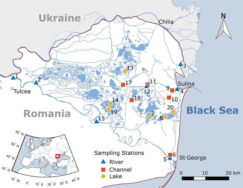
Figure 1. Sampling stations in the Danube Delta, Romania. Near long-term monitoring (see the Supplement). Although water
Tulcea, the Danube River splits into three branches, namely Chilia, temperature measured during summer months in both 2016
Sulina and St George. Station 16 was removed from the study and 2017 was up to 3 ◦ C warmer than the long-term mean,
because of limited access during lower water level (clogged ac- these values did not exceed the maximum temperatures mea-
cess channel). Shape files for map creation in QGIS are adapted sured in the last 20 years.
from https://mapcruzin.com/ (last access: 13 December 2016). Con-
tains information from https://www.openstreetmap.org/, which is 2.1.2 Categorization into river branches, channels and
made available under the Open Database License (ODbL) at https: lakes
//opendatacommons.org/licenses/odbl/1.0/.
We categorized our sampling stations into three groups
based on geomorphological characteristics, namely main
of the larger lakes of the Danube Delta have been subject to river branches, lakes and channels. River branch stations are
CO2 and CH4 evasion studies in the past (Durisch-Kaiser et all located along the three main branches of the Danube
al., 2008; Pavel et al., 2009), the main branches of the river River, exhibiting velocities of about 0.75 m s−1 (Danube
and the small channels are considered unchartered territory Commission, 2018), large hydraulic cross sections and fre-
with respect to CO2 and CH4 concentrations and fluxes. quent embankments. The category of lake refers to shallow
(2–3.5 m) open-water bodies within reed bed areas, and five
2.1.1 Hydrology
out of six sampling stations showed abundant macrophytes
The hydrology of the Danube River, which drives water ex- in summer. Natural and artificial channels represent the third
change with the delta, has a pronounced seasonality. Receiv- category. They provide a surface water connection between
ing meltwater from the Alps and Carpathians, the Danube the lakes and the river branches. We included old meanders
shows peak discharge in spring from April to June (Fig. 2), of the Danube and small channels within the delta. Both of
whereas the discharge minimum occurs in autumn from these features show a low flow velocity of up to 0.3 m s−1 ,
September through November. December and January often yet span quite a range in terms of surface area and depth. Ac-
show a small peak in discharge. The discharge provided by cessibility by motor boat determined the sampling stations in
the Danube River drives the seasonal and annual hydrolog- lakes and channels and restricted our monitoring to deeper
ical changes in the delta. From 2000 to 2014, the Danube’s lakes and larger channels. Both lakes and channels are con-
average annual discharge was 6760 m3 s−1 (ICPDR, 2018), nected to adjacent reed beds and marsh areas. Very shallow
which is a 3 % increase compared to the period from 1930 or isolated lakes, which are not represented in our data set,
to 2000 (Oosterberg et al., 2000). In the delta region, the may receive a significant part of their water from adjacent
discharge splits into the different main branches as follows: reed beds (Coops et al., 2008) and have a higher residence
Chilia – 53 %; Sulina – 27 %; St George – 20 % (ICPDR, time of up to 300 d compared to the investigated lakes, which
2018). Approximately 10 % of the Danube’s total discharge have an estimated residence time of 10–30 d (Oosterberg et
(620 m3 s−1 ; averaged over 1981–1990) flows through the al., 2000).
delta, of which about 20 % (120 m3 s−1 ) is lost via evapo-
transpiration (Oosterberg et al., 2000).
To assess the hydrological conditions during the time of
observation with respect to the long-term average, we com-
pared water level observations from Isaccea, Romania (IN-
https://doi.org/10.5194/bg-18-1417-2021 Biogeosciences, 18, 1417–1437, 2021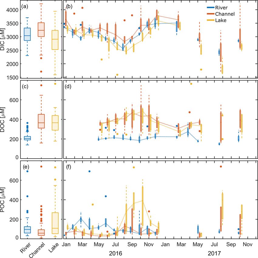
1420                              M.-S. Maier et al.: Spatio-temporal variations in lateral and atmospheric carbon fluxes

2.2     Sampling                                                 introduced with the air during equilibration. As tests showed
                                                                 that there was no significant difference between the lab- and
Our research area was located in the southern part of the        field-based methods (see the Supplement), we pooled the
delta enclosed by the Sulina and St George branches, which       data in our analysis.
we studied intensively in 2016 and 2017. We focused on              CO2 concentrations were measured in the field using a sy-
the southern part of the delta, since it is less impacted by     ringe headspace equilibration of 30 mL sampling water with
agriculture compared to the area north of the Sulina branch      30 mL air. The syringes were shaken for 2 min and allowed
(Niculescu et al., 2017). Samples and in situ measurements       to equilibrate before the transfer of the headspace into a dry
were taken once per month at 19 stations (Fig. 1), repre-        syringe and analysis in an infrared gas analyser (EGM-4; PP
senting river main branches (n = 7), channels (n = 6) and        Systems). The method is explained in more detail in Teodoru
the larger delta lakes (n = 6). The sampling stations in the     et al. (2015).
channels and lakes cover both the fluvial (west of station 18;      Dissolved O2 concentration was measured in situ using
Fig. 1) and the fluvio-marine parts of the delta. In situ mea-   a YSI ODO probe. The sensor was calibrated daily using
surements and sampling with a Niskin bottle was carried out      water-saturated air and cross-checked with oxygen readings
50 cm below the water surface. Sample analyses were con-         from a YSI Pro Plus multimeter sensor. We measured local
ducted at the Eawag laboratories in Switzerland.                 in-stream respiration rates to evaluate if community respira-
                                                                 tion could sustain our measured CO2 fluxes. The respiration
2.3     Dissolved and particulate carbon species                 rate was measured as O2 drawdown over a 24 h period. For
                                                                 the measurement, six biological oxygen demand (BOD) bot-
For DIC measurements, filtered (0.2 µm) and bubble-free wa-
                                                                 tles were filled with water samples, and three were measured
ter samples were stored in 12 mL Labco Exetainers under
                                                                 immediately afterwards at t = 0. The other three bottles were
cool and dark conditions until analysis with a Shimadzu
                                                                 stored in the dark at approximately in situ temperatures, and
TOC-L analyser. For the analysis of POC and DOC, water
                                                                 the O2 concentration was measured after 24 h. The O2 con-
was filtered through 7 µm pre-combusted and pre-weighed
                                                                 sumption rate was derived from the time and concentration
Hahnemühle glass fibre (GF) 55 filters. The filters were
                                                                 difference, assuming a linear decrease over time. We used
stored at −20 ◦ C until analysis, when they were dried and
                                                                 this respiration rate to estimate the local CO2 production rate
weighed for total suspended matter, subsequently fumigated
                                                                 by assuming a 1 : 1 aerobic respiration relation of O2 : CO2 .
with HCl for 24 h to remove the inorganic fraction and anal-
                                                                 Ward et al. (2018) argue that respiration rate measurements
ysed by EA-IRMS (elemental analyser) for organic carbon
                                                                 in BOD bottles underestimate the respiration rate because
content, which we used to calculate POC. The filtered water
                                                                 microbial processes are limited by both the bottle size and
was acidified using 100 µL 10M HCl and stored in the dark at
                                                                 the lack of turbulence, and they suggest a correction factor of
4 ◦ C until the analysis of DOC with a Shimadzu TOC-L anal-
                                                                 2.7 to correct BOD-derived respiration rates for size effects
yser. Due to potential contamination during sampling, DOC
                                                                 only or a factor of 3.7 for size and low turbulence effects. Ap-
data prior to May 2016 was discarded.
                                                                 plying these correction factors did not change the main point
2.4     Dissolved gases                                          of our comparison between fluxes and CO2 production rates.

2.4.1    Concentration measurements                              2.4.2   CO2 and CH4 flux measurements

We used mostly field-based methods for the analysis of           CO2 and CH4 fluxes were measured using a floating cham-
dissolved CH4 , CO2 and O2 . In 2016, samples for CH4            ber. The chamber had an internal area of 829.6 cm2 and an
analysis were taken for laboratory-based analysis by gas         internal volume of 10 080 cm3 , leading to a volume/area ra-
chromatography. Bubble-free water was filled into 120 mL         tio of 12.15 cm. An aluminium foil coating minimized heat-
septa vials by allowing an overflow of approximately three       ing during deployment. CO2 was routinely measured in the
times the sample volume before preserving the sample by          field over a 30 min period by coupling an infrared gas anal-
adding CuCl2 . Depending on the expected concentrations, a       yser (EGM-4; PP Systems) to the chamber in a closed loop.
headspace of 15–25 mL was created in the lab using pure N2 .     In 2016, CH4 was sampled from the chamber by syringe and
Samples were equilibrated overnight at 23 ◦ C on a shaker,       transferred overhead into 60 mL septa vials that had been
and the headspace was analysed using gas chromatography          pre-filled with a saturated NaCl solution until the liquid was
with a flame ionization detector (GC-FID; Agilent Technolo-      replaced by gaseous sample. These discrete samples for lab
gies, USA). In 2017, we used 1 L Schott bottles to prepare       analysis were taken at time t = 0, 10, 20 and 30 min and anal-
headspace equilibration directly in the field, using air. Sam-   ysed by GC-FID. In 2017, this laborious procedure was re-
ples were transferred to gasbags and analysed in the field for   placed by attaching the LGR analyser directly to the floating
CH4 using an Ultraportable CH4 / N2 O analyser (Los Gatos        chamber.
Research – LGR). We corrected for atmospheric contamina-            Flux chamber measurements were conducted, unless con-
tion during the processing by subtracting the amount of CH4      ditions were too windy or boat traffic was too frequent in

Biogeosciences, 18, 1417–1437, 2021                                                 https://doi.org/10.5194/bg-18-1417-2021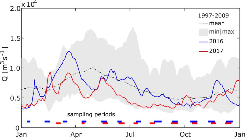
M.-S. Maier et al.: Spatio-temporal variations in lateral and atmospheric carbon fluxes                                     1421

the main channel. In total, we took 265 flux measurements          Raymond et al., 2013), we believe that median fluxes give
for CO2 and 122 for CH4 . Of the latter, 91 measurements           a more reliable representation of the fluxes in systems with
seemed to be without any significant influence of ebullition       large gradients. Based on the different characteristics of the
(i.e. R 2 of linear regression > 0.96; for more detail, see the    three waterscapes, we estimated the delta-scale atmospheric
Supplement) and are henceforth referred to as diffusive CH4        CO2 and CH4 fluxes by multiplying the median flux of each
fluxes. In the high-resolution LGR analyser time series, the       waterscape with its respective area (Table 1). We did this sep-
influence of gas bubbles could easily be identified. We cal-       arately for each month and summed up the results, consider-
culated the diffusive flux by fitting a linear regression to pe-   ing the respective number of days per month. For example,
riods where data showed no influence of ebullition. In this        the median annual flux from the rivers, F R , was calculated
case, the flux is calculated from the slope and the height of      as follows:
the gas volume in the chamber. In the discrete time series,
                                                                          12
it was hard to distinguish between diffusive flux and ebulli-             X
                                                                   FR =         FR,m × AR × ndays,m × 103 ,                   (3)
tion. When the linear regression of the discretely measured
                                                                          m=1
samples had an R 2 < 0.96, we considered the flux measure-
ment to be influenced by bubbles. In this case, we calculated      where FR,m is the median flux in mmol m−2 d−1 measured
the total flux by dividing the total concentration increase by     in the river stations in month m, AR is the area of the river
the observation time, as we did to calculate the total flux of     branches in square kilometres (see Table 1) and ndays,m rep-
the LGR analyser measurements. A total of three cases with         resents the respective number of days per month m. The fac-
R 2 > 0.96 showed fluxes > 20 mmol m−2 d−1 and were thus           tor 103 is used to convert to the units of mol yr−1 . To ob-
also classified as total flux. Discrete time series showing a      tain the annual flux from the channels, F C , and the lakes,
non-monotonous course (n = 12) were excluded from fur-             F L , we proceeded in the same way. We converted the result-
ther processing. Missing monotony can have several expla-          ing annual fluxes of the different waterscapes from mol yr−1
nations, including sampling captured a bubble or a sample          to GgC yr−1 and GgCO2 eq yr−1 , with the latter assuming a
mix up.                                                            global warming potential for CH4 of 28 over 100 years, i.e.
                                                                   neglecting climate feedback (IPCC, 2013). The total annual
2.4.3    Calculation of k600
                                                                   water–air flux, F tot , from the delta was the sum of the fol-
We used our CO2 flux measurements to calculate the gas             lowing three fluxes:
transfer coefficient k600 as follows:
                                                                   F tot = F R + F C + F L .                                  (4)
                      FCO2
kCO2 =                                                      (1)    We also performed this calculation using 25 and 75 per-
        (pCO2 ,water − pCO2 ,air ) · KH,CO2
            kCO2                                                   centiles instead of the median to assess the upper and lower
k600 =                 1
                         ,                                  (2)    boundaries of our estimate.
       (ScCO2 /600)− 2                                                For a reliable upscaling of fluxes, we determined the sur-
where FCO2 is the flux of CO2 , pCO2 is the measured partial       face area of each waterscape as precisely as possible (Ta-
pressure of CO2 in water and air, respectively, and KH,CO2 is      ble 1). We estimated the area covered by the Danube’s
the solubility coefficient for CO2 according to Weiss (1974).      branches by refining publicly available shape files for Roma-
ScCO2 is the Schmidt number for CO2 , calculated based on          nia and Ukraine (https://mapcruzin.com/, last access: 13 De-
temperature (Wanninkhof, 1992). We estimated missing flux          cember 2016), using the OpenLayers Plugin in QGIS, which
measurements using the median k600 of the respective water         allowed a comparison of the shape file with satellite images.
type and the measured CO2 concentrations.                          We used the same procedure for the lakes and arrived at the
   Analogously, diffusive CH4 fluxes were estimated from           surface area reported by Oosterberg et al. (2000). Assessment
the individually calculated k600 , using the solubility coeffi-    of the surface area of the delta channels was more difficult
cient from Wiesenburg and Guinasso Jr. (1979), the mean            as many of the small channels are hard to identify on satel-
global atmospheric CH4 mole fraction of 1.84 parts per mil-        lite images. Generally, estimating the width of the channels
lion (ppm; Nisbet et al., 2019) and the Schmidt number for         is challenging due to emergent macrophyte coverage, which,
CH4 from Wanninkhof (1992). We attributed the difference           depending on the image quality, blends in with the adjacent
between this estimate and the total measured flux to ebulli-       reed. Instead of mapping the channels, we therefore used the
tion.                                                              overall channel length reported by Oosterberg et al. (2000)
                                                                   and assumed an average channel width of 19 m, which means
2.5     Upscaling atmospheric fluxes to delta scale                the resulting surface area is on the lower end. Especially the
                                                                   old, cut-off meanders of the Danube River (Dunarea Veche),
Spatial upscaling of heterogeneous and scarce data is very         which we also consider as belonging to the channel category,
difficult and handled in various ways in the literature. Like      do have a much larger width ranging on the order of 100–
other authors in a global context (Aufdenkampe et al., 2011;       200 m.

https://doi.org/10.5194/bg-18-1417-2021                                                    Biogeosciences, 18, 1417–1437, 2021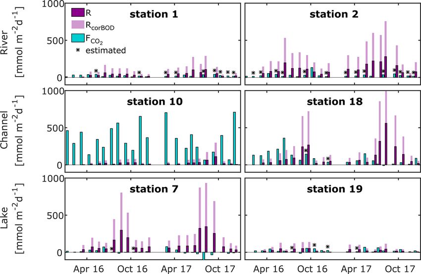
1422                                          M.-S. Maier et al.: Spatio-temporal variations in lateral and atmospheric carbon fluxes

Table 1. Surface area of the Danube Delta features. Assuming a 19 m channel width means the estimation of the surface area of the channels
is on the lower end. The surface areas of freshwater and wetland do not add up to the total area since parts of the delta are covered by forest
and agricultural polders.

   Feature                                                                   Area      Source
                                                                            (km2 )
   Freshwater                                                                 455      Sum of river branches, channels and lakes
   – River branches                                                           164      Extracted using QGIS∗
   – Channels                                                                  33      Length of canals from Oosterberg et al. (2000); 19 m width assumed
   – Lakes                                                                    258      Oosterberg et al. (2000); extracted using QGIS∗
   Wetland                                                                  3670       Mihailescu (2006)
   – Marsh vegetation (total)                                               1805       Sarbu (2006)
   – Scripo-Phragmitetum                                                    1600       Sarbu (2006)
   Agriculture, forest, settlements, pastures and fish ponds                1515       Total surface area – wetland; freshwater
   Total surface area within the three main branches                        3510       Niculescu et al. (2017)
   Total surface area of the delta                                          5640       Mihailescu (2006)
   Surface area of the Danube River catchment                             817 000      Tudorancea and Tudorancea (2006)
∗ This is based on shape files adapted from https://mapcruzin.com/ (last access: 13 December 2016) and contains information from https://www.openstreetmap.org, which is made
available under the Open Database License (ODbL) at https://opendatacommons.org/licenses/odbl/1.0/.

2.6    Import by the Danube River and export to Black                                     Stations 4 and 5 are located slightly upstream of the settle-
       Sea                                                                                ments of Sulina and St George to avoid measuring the effect
                                                                                          of these two settlements. Station 3 is located in a small side
To compare the delta’s CO2 and CH4 emissions to the lateral                               arm of the Chilia branch, marking the border between Roma-
transfer of carbon from the catchment to the Black Sea and                                nia and Ukraine, which, during comparison measurements,
the influence of the delta region, we also calculated the loads                           showed the same water composition as the main branch.
of dissolved and particulate carbon species transported by the                               In our data processing, we decided to exclude one unusu-
Danube at the delta apex, FD , and close to the Black Sea,                                ally high POC value in April at the Sulina branch (station 4)
FBS . As a first step, we calculated the daily average load of                            from our load calculation as we assume it is caused by a high-
each month, Fm , for the different carbon species, as follows:                            discharge, high-turbidity event that does not represent the
                                                                                          monthly mean well. Instead, we interpolated between March
Fm = Cm · Qm ,                                                                 (5)        and May. For DOC, we replaced missing data from January
where Cm is the concentration of DIC, DOC or POC mea-                                     to April 2016 with the measurements at the same stations in
sured in month m, and Qm is the respective averaged daily                                 2017, assuming that they are also good estimates for the pre-
discharge of month m. Since CH4 showed much smaller con-                                  vious year. This way, we arrived at DOC estimates that cover
centrations (∼ factor 100–1000 with respect to DOC and                                    the same period as DIC and POC.
DIC), we did not include it into the calculation. In a sec-                                  We calculated the lateral transfer of carbon between the
ond step, we weighed Fm by the number of days per month,                                  Danube Delta and its river, Flateral , by subtracting the load
ndays,m , and took the sum over all the months of the year. The                           exported to the Black Sea via the three main branches, FBS ,
load transported by the Danube River upstream of the delta,                               from the load imported to the delta from the catchment, FD ,
FD , was calculated based on the concentrations measured at                               as follows:
station 1 (Fig. 1), which is located in the Tulcea branch close                           Flateral = FD − FBS .
to the apex of the delta and represents the water signature
from the catchment, as follows:                                                           The resulting lateral flux, in our case, is comparably small,
         12
                                                                                          and we used Gaussian error propagation to estimate its range.
                                                                                          The basis for the error propagation was the measurement un-
         X
FD =          Fm (st.1) × ndays,m .                                            (6)
        m=1                                                                               certainties in the concentrations (0.5 % DIC; 4 % DOC; 10 %
                                                                                          POC) and discharge (3 %, assumed), which were used to cal-
Data from the stations in the three main branches close to                                culate the loads.
the Black Sea (stations 3, 4 and 5; Fig. 1) were used to esti-
mate the amount of carbon exported to the Black Sea, FBS ,                                2.7     Statistical analysis
as follows:
                                                                                          We used MATLAB R2016a and R2017b for the statistical
         12
FBS =
         X
               [Fm (st.3) + Fm (st.4) + Fm (st.5)] × ndays,m .                 (7)        analysis of the data set. The data were evaluated for normal
         m=1
                                                                                          distribution, using histograms and quantile-quantile plots. In

Biogeosciences, 18, 1417–1437, 2021                                                                                https://doi.org/10.5194/bg-18-1417-2021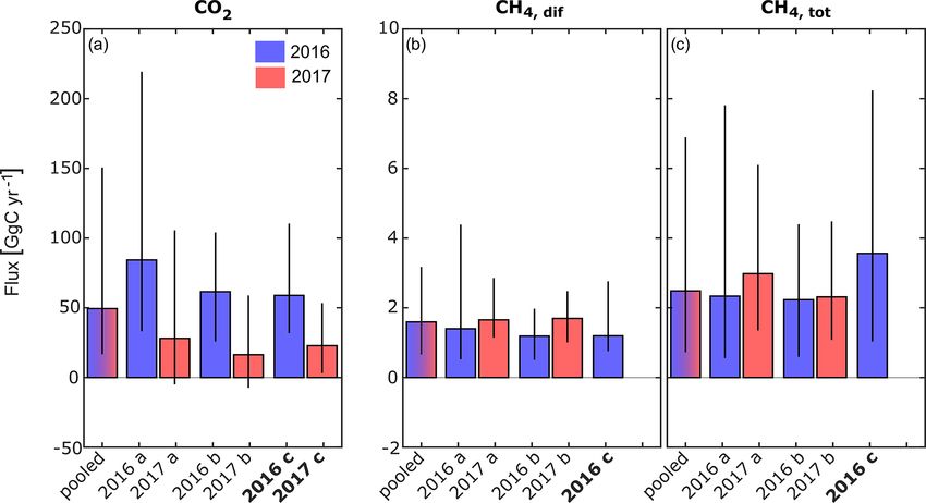
M.-S. Maier et al.: Spatio-temporal variations in lateral and atmospheric carbon fluxes                                      1423

                                                                     increasing trend from May to October 2016, but in the river,
                                                                     concentrations already peaked in July 2016 and were low-
                                                                     est in October. Median concentrations were quite compara-
                                                                     ble for 2017, with a tendency towards lower values. DOC in
                                                                     the main river in August 2017 was nearly 30 % lower than
                                                                     in the previous year. Most of the year, DOC concentrations
                                                                     were nearly a factor 10 smaller than measured DIC concen-
                                                                     trations.
                                                                        In 2016, we observed the lowest median POC concentra-
                                                                     tion in the channels (Fig. 3e, f). Median concentrations in
                                                                     both rivers and lakes were nearly twice as high compared to
                                                                     channels but showed a distinctly different seasonality. POC
Figure 2. Daily average discharge close to the apex of the Danube    was highest in the main river from March to June, while it
Delta. The dotted line and the shaded area show mean and minimum     peaked in lakes during August to October, suggesting differ-
to maximum daily discharge, respectively, for the period from Jan-   ent carbon sources.
uary 1997 to October 2009 at Reni, Ukraine (ICPDR, 2018). Blue
and red lines show daily average discharge at Isaccea, Romania, in   3.2     Dissolved gases
2016 and 2017 (INHGA; Feodorov). Horizontal bars indicate the
timing of sampling campaigns. The x axis ticks indicate the 15th
                                                                     3.2.1    Concentrations
day of the respective month.
                                                                     During the entire monitoring period, CH4 in water samples
                                                                     of the delta was always oversaturated with respect to atmo-
case of O2,sat , CH4 and POC, data distribution improved to-
                                                                     spheric equilibrium concentrations of 0.0046 to 0.0023 µM
wards normality using log transformation; however, the re-
                                                                     at T = 0 to 30 ◦ C (Fig. 4c, d). Median concentrations
sults were not fully satisfying. Levene’s test revealed, fur-
                                                                     in the river samples were thus ∼ 100 times oversaturated
thermore, the heteroscedastic nature of our data. Results for
                                                                     (0.33 µM). The channels exhibited a more than 3 times higher
tests of significant difference between the three aquatic cat-
                                                                     median concentration than the main river (1.1 µM), with the
egories, from the non-parametric Kruskal–Wallis test (De
                                                                     highest concentrations in July to September 2016 (up to
Muth, 2014) followed by a multiple comparison test after
                                                                     59 µM). In contrast, the median concentration in the lakes ex-
Dunn–Sidak, were therefore taken very cautiously. Given the
                                                                     ceeded the value of the main river only slightly (0.43 µM) yet
non-normality of the data, we report median instead of mean
                                                                     with a much larger range. In all three subsystems, concentra-
values and give ranges as 25 to 75 percentiles or minimum to
                                                                     tions increased from February 2016 to maximum values in
maximum measured values, as indicated.
                                                                     July to October 2016. In 2017, concentrations were lower in
   Box plots shown in this paper indicate the 25 and 75 per-
                                                                     the channels compared to 2016.
centiles and the median. Outliers are detected using the in-
                                                                        Similarly to CH4 , we found CO2 concentrations to be con-
terquartile range (> 1.5 × IQR). The whiskers indicate the
                                                                     stantly supersaturated with respect to the atmosphere in the
minimum and maximum values that are not detected as out-
                                                                     main branches of the Danube, ranging from 26 to 140 µM
liers by this procedure.
                                                                     (Fig. 4e, f). The median concentration of 59 µM was more
                                                                     than 3 times as high as the equilibrium concentration of
3     Results                                                        CO2 at 15 ◦ C (18.2 µM). Channels showed a much higher
                                                                     range (2.4 to 790 µM), with a significantly higher median of
3.1    Dissolved and particulate carbon species                      140 µM. During the entire monitored period, we encountered
                                                                     undersaturated conditions in this class at only two stations
DIC concentrations measured during our study ranged from             (17 and 18) in August 2017. Lakes, however, were undersat-
1.6 to 4.2 mM (Fig. 3a). Median DIC concentrations were              urated on 11 occasions in 2016 and 32 occasions in 2017.
around 3.0 mM over the whole observation period, with                Dissolved concentrations in this category ranged from 0 to
channels showing 10 % higher and lakes showing 3 % lower             95 µM, with a median of 28 µM.
median concentrations than the main river. In 2016, concen-             In 2016, CO2 concentration showed a pronounced season-
trations were lowest in August and highest in December in            ality in all three subsystems. In the main river, median CO2
all three groups (Fig. 3b). In 2017, median concentrations           nearly doubled from January 2016 to April 2016 and sub-
were 10 % (rivers) to 20 % (channels and lakes) lower than           sequently decreased to reach levels around 60 µM. In 2017,
in 2016.                                                             no clear seasonal pattern emerged. That year, median values
   DOC levels in the delta were about 1.8 times the concen-          mostly ranged around 60 µM, with the lowest median con-
trations observed in the river (Fig. 3c, d). Channels and lakes      centration recorded in June (44 µM) followed by the maxi-
had very similar concentrations, and both showed a general           mum in July (81 µM).

https://doi.org/10.5194/bg-18-1417-2021                                                        Biogeosciences, 18, 1417–1437, 2021
1424 M.-S. Maier et al.: Spatio-temporal variations in lateral and atmospheric carbon fluxes Figure 3. Measured DIC, DOC and POC concentrations in the different waterscapes (river, channel and lake). (a, c, e) The 2-year observation period. (b, d, f) Seasonality of the data. Dotted lines connect median values. The x axis ticks indicate the 15th day of the respective month. Box plots indicate 25 and 75 percentiles and median; whiskers indicate maximum and minimum, with data > 1.5 × IQR shown as outliers. Channels showed the largest increase in CO2 during the longer period, from March to December, in the drier year of warm season. Median concentrations increased more than 2017. In 2016, lakes showed highest median CO2 concentra- 4 times, from 66 µM in February 2016 to 290 µM in July tions in April (74.4 µM) and the lowest concentrations in July 2016. In terms of inter-annual CO2 variability, 2017 showed and August (20.5 and 14.6 µM, respectively). With the con- a later and less pronounced increase in concentration (72 µM centration increase in early spring, the decrease in summer in March to 187 µM in May), followed by an earlier de- and the following increase in autumn, the seasonal signal in cline than 2016. From August 2017 to November 2017, me- 2016 recalls a sinusoidal curve. The pattern in the drier year, dian monthly concentrations ranged around 50 µM and were 2017, however, showed less variation with lower concentra- lower than the concentrations in the main river during this tions which were ranging from 0 to 71 µM. period. In general, CO2 concentrations in the channels in O2 saturation, as one might expect, often showed a mirror 2017 were 18 % to 75 % below the values observed in 2016. image to the CO2 time series in all three systems (Fig. 4g, h). We found the highest concentrations in the eastern part of The main river was generally slightly undersaturated, with the delta (station 10; Fig. 1), where concentrations reached a median O2 saturation of 93 %. O2 saturation in river wa- around 360 µM in winter and up to 785 µM in summer 2016. ter ranged between 75 % and 109 % during the whole obser- Compared to rivers and channels, lakes generally had the vation period. Median saturation in the channels was 14 % lowest CO2 concentrations and showed a distinctly differ- lower (79.5 %) and – as for CO2 – covered a much broader ent seasonal pattern. Most of the observed lakes (stations 7, range than in the main river. The lowest values observed 8, 13 and 14) were undersaturated in the period from May were as low as 5 % O2 saturation (0.4 mg L−1 ) in July 2016, to November 2016. CO2 undersaturation in these lakes (in- while maximum saturation reached nearly 150 % in August cluding station 20) occurred 3 times more often and over a 2017. In winter, O2 saturation in the channels was compa- Biogeosciences, 18, 1417–1437, 2021 https://doi.org/10.5194/bg-18-1417-2021
M.-S. Maier et al.: Spatio-temporal variations in lateral and atmospheric carbon fluxes 1425
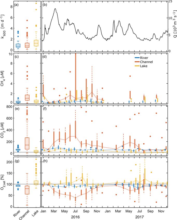
Figure 4. Here, k600 (a), daily average discharge close to the apex (b) and measured concentrations of dissolved gases in the different
waterscapes, i.e. river, channel and lake (c–h), are shown. (a, c, e, g) Pooled data from 2 years. (d, f, h) Seasonal dynamics, with dotted
lines connecting median values. The x axis ticks indicate the 15th day of the respective month. (c, d) CH4 in 2016, with four channel
values (ranging from 22.2 to 58.0 µM) and one lake station (12.5 µM) exceeding 10 µM cut off. (e, f) Dotted black line represents the
equilibrium concentration of CO2 at 15 ◦ C (18.2 µM). Box plots indicate the 25 and 75 percentiles and median; whiskers indicate maximum
and minimum, with data > 1.5 × IQR shown as outliers.
rable with the river stations. Station 10 showed an excep- 3.2.2 Measured atmospheric CO2 and CH4 fluxes
tional behaviour and never exceeded a saturation of 72 % or
9 mg L−1 . O2 saturation in the channels strongly decreased in Median CO2 fluxes were largest in channels
the spring and summer months, resulting in concentrations of (93 mmol m−2 d−1 ; see Table 2) where we also observed
less than 2 mg L−1 at station 9 in July 2016 and at station 10 the highest overall flux of 880 mmol m−2 d−1 . Lakes were
from July to September 2016 and in June, July and October the only locations that showed significant negative fluxes,
2017. Contrastingly, most lakes showed a strong oversatu- i.e. CO2 uptake during summer, when O2 was strongly
ration of up to 180 % from April to October, resulting in a oversaturated.
median saturation that slightly exceeded 100 %. The highest median diffusive fluxes of CH4 were ob-
served in the channels with 1.1 mmol m−2 d−1 . Diffusive ef-
flux from the river was generally lowest, while the lakes
https://doi.org/10.5194/bg-18-1417-2021 Biogeosciences, 18, 1417–1437, 20211426 M.-S. Maier et al.: Spatio-temporal variations in lateral and atmospheric carbon fluxes
Table 2. Median and range of measured CO2 and CH4 fluxes (mmol m−2 d−1 ) and calculated k600 values (m d−1 ). Additionally, n states
the number of measurements. The range indicates the minimum and maximum observations.
Parameter River Channel Lake
Median Range n Median Range n Median Range n
FCO2 25 7.3–150 57 93 −9.7–880 105 5.8 −110–160 103
FCH4 ,tot 0.42 0.056–2.7 21 2.0 0.062–51 47 1.5 0.031–47 54
a
FCH 0.37 0.056–2.7 17 1.1 0.16–6.2 34 0.82 0.031–6.7 40
4 ,dif
b
k600 0.69 0.20–3.4 57 0.74 0.11–5.4 103 1.2 0.13–8.6 96
a The data in this table rely only on measured F
CH4 ,dif . Missing diffusive CH4 fluxes for the upscaling were calculated from k600 .
b Measurement uncertainty led to negative k
600 values in nine cases (i.e., twice in the channels and seven times in the lakes). These values
were deleted manually; thus, n(k600 ) is < n(FCO2 ) for channels and lakes.
showed the largest variability, with a minimum of 0.03 and a 3.3 Upscaling atmospheric fluxes to delta scale
maximum of 6.7 mmol m−2 d−1 . Considerable ebullition oc-
curred only in the delta lakes and channels, which accounted The upscaling of the freshwater CO2 and CH4 fluxes to the
for ∼ 70 % of the total CH4 flux. freshwater surface of the delta according to Eq. (4) led to a
The gas transfer coefficient, k600 , was calculated from the net CO2 flux of 60 GgC in 2016 and less than half (23 GgC)
measured CO2 fluxes. Median k600 was lowest in the river in the drier year of 2017 (Figs. 6 and 7a; case “c”) when the
branches and in the channels at 0.69 and 0.74 m d−1 , respec- overall contribution of the three compartments was lower and
tively (see Table S1). As lakes were more exposed to wind, lakes turned into a net sink. The diffusive CH4 flux (Fig. 7c)
median k600 was considerably higher (1.2 m d−1 ), and we ob- was 1 order of magnitude smaller than the CO2 flux (Fig. 7a),
served the maximum k600 of 8.6 m d−1 in this category. but it increased three-fold when ebullition was considered
(Fig. 7d).
3.2.3 CO2 production rate vs. CO2 flux Especially the CO2 fluxes seem to be subject to consid-
erable inter-annual variability (Fig. 7a, b), which highlights
We find respiration rates ranging between 0.8– the need to discriminate between different years during the
390 mmol m−2 d−1 for rivers, while in the channels upscaling process. It is likely that the different hydrological
and lakes they ranged from 2.3–560 mmol m−2 d−1 conditions triggered different amounts of lateral inflow from
and 1.0–350 mmol m−2 d−1 , respectively (Figs. 5 and the reed-covered wetlands and contributed to the large vari-
S7–S9). Median respiration rate is highest in rivers ability in CO2 fluxes. For CH4 , this effect appears to be much
(54 mmol m−2 d−1 ), followed by lakes (48 mmol m−2 d−1 ) smaller.
and channels (45 mmol m−2 d−1 ). Many stations showed a Considering the contributions from the different water-
pronounced seasonality, with the highest respiration rates scapes shows that the river branches were the main source
occurring mostly between July and October. Respiration of CO2 to the atmosphere in both years (Fig. 6a, b). Despite
rates, i.e. CO2 production rates, generally exceed CO2 fluxes their small surface area (7 %), channels contributed 32 %–
in river and lake stations throughout the year (Fig. 5), which 37 % to the total CO2 flux. Lakes, on the other hand, switched
implies that local instream CO2 production sustained the from a net CO2 source of 19 GgC in 2016 to a small net CO2
observed fluxes. At the channel stations, we frequently sink of −3.3 GgC in the drier year of 2017. In 2016, the lakes
observed fluxes exceeding the local production, even if we emitted the largest share of CH4 , with 66 %, considering only
account for the potential underestimation of the CO2 pro- diffusive fluxes (Fig. 6c), and 86 %, considering total CH4
duction, which implies the presence of other CO2 sources. fluxes (Fig. 6d). Considering the global warming potential of
This was most striking at station 10, the CO2 hot spot, where CH4 (IPCC, 2013), CH4 was responsible for 17 % of the total
CO2 outgassing exceeded local respiration on average by a 260 GgCO2 eq yr−1 emitted in 2016.
factor of 40. At the other channel stations (also see Fig. S8),
there seems to be a seasonally occurring pattern. CO2 fluxes
3.4 Lateral carbon transport
exceed local production in the first half of the year, while
they fall below local production for the remainder of the
The annual import of carbon to the apex of the delta amounts
year. While this pattern is very distinct in 2016, it is less
to 8490 ± 240 GgC yr−1 (Fig. 8). This flux consists mostly
pronounced in the drier year of 2017, which suggests that
of inorganic carbon (DIC; 91 %), while DOC and POC com-
the additional CO2 source is linked to hydrology.
prise only small fractions of 6 % and 3 %, respectively. Lat-
eral fluxes are highest in spring when discharge is highest.
About 10 % of the Danube’s water is channelled into the delta
Biogeosciences, 18, 1417–1437, 2021 https://doi.org/10.5194/bg-18-1417-2021M.-S. Maier et al.: Spatio-temporal variations in lateral and atmospheric carbon fluxes 1427 Figure 5. Flux rate and production rate of CO2 , as calculated from O2 community respiration incubations, for selected river, channel and lake stations. Fluxes marked with asterisks were calculated from median k600 of our observations in the respective waterscape. Dark purple bars represent measured respiration rates; light purple bars indicate the effect of a correction for measurement limitations using BOD bottles (factor 2.7; see Ward et al., 2018). Figure 6. Annual greenhouse gas fluxes to the atmosphere obtained by upscaling the monthly median flux to the total area of each waterscape and taking the sum over all months (see text for details). Black vertical lines indicate the uncertainty and were calculated using the 25 percentile and 75 percentile, respectively, instead of median values for the calculation. CO2 flux in panels (a) 2016 and (b) 2017. (c) Diffusive and (d) total CH4 flux in 2016. Due to large data gaps, this calculation was not done for CH4 in 2017. All fluxes are in GgC yr−1 . For tabulated values, see Table S2. before reaching the Black Sea (Oosterberg et al., 2000); thus, flow load reaching the apex of delta. The slightly higher load we assume that 10 % of the annual carbon load of the Danube mainly relates to increased DOC levels reaching the main reaches the delta (i.e. 849 GgC yr−1 ). branches from the delta, especially during the spring flood in The water export from the delta, however, is poorly con- March and April. The relatively small fraction of water that strained. The balance between precipitation minus evapo- passes through the delta changes the relative fraction of DOC ration is negative, poorly quantified and quite variable. We and POC only marginally to 7 % and 4 %, respectively, while therefore rely on the flux balance of the three branches to es- the largest fraction in the water reaching the Black Sea re- timate carbon export from the delta. The resulting export to mains DIC (89 %; Fig. 8). DIC import and export is fairly the Black Sea via the Danube’s main branches amounts to comparable throughout the year, while POC export to the 8650 ± 150 GgC yr−1 and is less than 2 % higher than the in- Black Sea strongly exceeded the imports from the catchment https://doi.org/10.5194/bg-18-1417-2021 Biogeosciences, 18, 1417–1437, 2021
1428                                 M.-S. Maier et al.: Spatio-temporal variations in lateral and atmospheric carbon fluxes

Figure 7. Comparison of greenhouse gas fluxes from the delta’s freshwaters to the atmosphere obtained by the different upscaling approaches,
i.e. pooled, and cases “a” (discrimination by year), “b” (discrimination by year and waterscape) and “c” (discrimination by year, waterscape
and month). Black vertical lines indicate the uncertainty when performing calculations using the 25 and 75 percentiles instead of median
values. (a) CO2 flux. (b) Diffusive and (c) total CH4 flux. All fluxes are in GgC yr−1 . Bold y axis labels indicate the calculation approach
(case “c”), which is shown in more detail in Fig. 6 for the individual contributions from rivers, channels and lakes.

in April. DOC exports are highest in the first half of the year          jdgeest et al., 2016; Zurbrügg et al., 2012). The large differ-
(see Fig. S5).                                                           ence between the waterscapes, with respect to CO2 and CH4
                                                                         fluxes, supports our approach to treating the waterscapes in-
                                                                         dependently when upscaling the flux measurements to the
4     Discussion                                                         total water surface of the delta.

4.1    The main waterscapes of the Danube Delta                          4.2     Dominating processes

                                                                         4.2.1    River branches
As we had hypothesized, carbon dynamics differed sig-
nificantly across the three different waterscapes. The non-              The main river branches of the Danube are mostly influenced
parametric Kruskal–Wallis test, followed by the Dunn–Sidak               by the hydrology and chemistry of the catchment, as shown
test, showed that the median of the three classes is signif-             by the comparison between the concentrations at the delta
icantly different for concentrations of CH4 , CO2 , O2 and               apex with concentrations in the three main branches close to
DIC (see the Supplement). In the case of DOC, only the                   the Black Sea. There is comparably little variation between
rivers differ significantly from the other two groups, while             the stations with respect to DIC, DOC and POC. At all sites,
in the case of POC, only channels are significantly differ-              O2 is slightly undersaturated most of the time, but we do not
ent. Rivers and lakes, however, may differ significantly in              see a strong influence of the delta close to the Black Sea.
the quality of their POC, as observed by the seasonality of
the signal, which shows that high POC in the river actually              4.2.2    Channels
occurs during high discharge in spring, while high POC in
the lakes occurs during algal blooms in late summer. The                 Carbon dynamics in the channels are strongly affected by the
non-parametric Kruskal–Wallis test does not require normal               water source. The channels are connecting the river branches
distribution of the data, but it requires equal variance of the          to the delta lakes. The direction of this connection depends
data groups investigated for the difference in median (Hed-              primarily on hydrologic gradients between the delta and the
derich and Sachs, 2016). Our observations in the seasonal                main branches, which means that flow direction can reverse
plots (Figs. 3, 4) support the results of the test. In most cases,       in individual channels and, thus, alter their chemical signa-
the box plots do not overlap, indicating that the three groups           ture due to a change in the main inflow. Seasonally, the chan-
are significantly different. For example, DOC is significantly           nels transport dissolved carbon into the delta and provide
higher in the delta lakes and channels due to the strong pri-            nutrients to the reed stands during the high-water season.
mary productivity of these systems. O2 is significantly lower            During times of receding water levels in the main branches,
in the channels than in the other two categories due to the lat-         the channels act as the delta’s drainage pipes. The compar-
eral inflow of oxygen-depleted waters from the wetland (Zui-             ison between CO2 fluxes and local CO2 production rates

Biogeosciences, 18, 1417–1437, 2021                                                          https://doi.org/10.5194/bg-18-1417-2021
M.-S. Maier et al.: Spatio-temporal variations in lateral and atmospheric carbon fluxes 1429
(Fig. 5) shows that the high CO2 fluxes in the channels are
often not sustained by in-stream respiration alone, in con-
trast to what we observed in the river and lakes. While this
discrepancy mainly occurs during high discharge in spring,
it is most evident at station 10, where it occurs throughout
the year of 2016. Station 10 is located in Canalul Vatafu-
Împutita, Romania, at the border of a core protection zone
of the biosphere reserve. During this study, it stood out as a
CO2 hot spot, responsible for the highest CO2 concentrations
(Fig. 4f). Additional CO2 -rich water inflows from adjacent
wetlands could explain the large CO2 fluxes, which exceed
CO2 production. The water at station 10 was always excep-
tionally clean, low in oxygen content and had a low pH, sup-
porting the hypothesis of a pronounced input from the reed
beds. During times of unusually low water levels, such as
in August and September 2017, the lateral influx from the
reed seems to cease (Fig. 5). The, at first glance, contradic- Figure 8. Overview of carbon flux estimates in GgC yr−1 . The to-
tory timing of the increased lateral inflow during increasing tal area between the main branches is 3510 km2 (see Table 1). Black
water levels at the other channel stations could be explained and grey numbers refer to fluxes estimated during this study based
by a pressure wave. Water flooding the vegetated area in the on data from 2016. The following italicized values refer to esti-
west will push out old water with a long residence time in mates based on the data in the literature from different study pe-
the vegetated area at the other edges further east. In general, riods (studies for carbon burial and primary production do not ex-
plicitly consider seasonality): ∗ carbon burial in lakes, based on av-
channel water in the Danube Delta is therefore a mixture of
erage sedimentation rate measured in seven lakes in the Danube
three main sources, namely Danube river water, lake water
Delta, with an organic carbon content range of 3 %–30 % (Begy
and water infiltrating from the wetland. The importance of et al., 2018); ∗∗ net CO2 uptake of Phragmites australis upscaled
the individual water source depends on the location of the to the area covered by the Scripo-Phragmitetum plant community
channel sampling sites and on the water levels, which trigger (Zhou et al., 2009); ∗∗∗ upscaled primary productivity of the Scripo-
flooding or draining conditions. Phragmitetum plant community (Sarbu, 2006). The green area in
the plot symbolizes the reed area without indicating all the loca-
4.2.3 Lakes tions of its occurrence.
In the lakes, residence times of 10–30 d allow primary pro-
duction and local decomposition of organic matter to become atmosphere (Zhang et al., 2018). Potamogeton crispus, for
important factors driving carbon cycling. We observed abun- example, which is also found in the delta lakes and chan-
dant macrophytes like Ceratophyllum demersum and Elodea nels, seasonally sustained CH4 fluxes that were up to 3
canadensis growing in spring and early summer, which, de- times higher than CH4 fluxes from Ceratophyllum demersum
pending on lake depth, even reached the lake water surface. (Zhang et al., 2018). Studies showed that the plant commu-
A change in the abundance of submerged vegetation to veg- nity composition in the delta lakes shifted since the 1980s
etation with floating leaves might be linked to changes in the due to increasing eutrophication, which also led to an in-
CO2 and CH4 fluxes (Grasset et al., 2016). Around July, al- crease in Potamogeton species recorded in the delta (Sarbu,
gal blooms coincided with a significant reduction in macro- 2006). It remains unresolved whether this change in vegeta-
phyte abundance. This pattern seems to be reoccurring due tion also affected the CH4 release in the Danube Delta.
to the eutrophic state of the delta lakes (Tudorancea and
Tudorancea, 2006; Coops et al., 2008, 1999). During our 4.3 Uncertainties linked to the upscaling procedure
observations, both macrophytes and algal blooms caused a
drawdown of CO2 and supersaturation in O2 (Fig. 4f, h). 4.3.1 Spatial heterogeneity
The algal blooms also partly explain the peak in measured
POC from July to November, which extended to most of the In a hydrologically complex system like the Danube Delta,
delta’s channels (Fig. 3f). The degradation of the macrophyte upscaling CO2 and CH4 is prone to several sources of uncer-
biomass coincided with locally elevated CH4 concentrations tainties, most of them linked to the delta’s small channels and
from July to October (Fig. 4d). lakes. First, the channel category showed a large range, not
In constructed wetlands, macrophytes were found to influ- only in DOC and POC concentrations but also in dissolved
ence the composition of methanogenic communities by af- gases and their fluxes. We attribute this primarily to the vary-
fecting dissolved O2 and nitrogen in the rhizosphere, which ing contribution from the three different water sources, with
had a direct impact on the amount of CH4 released to the lateral influx from the reed stands drastically increasing the
https://doi.org/10.5194/bg-18-1417-2021 Biogeosciences, 18, 1417–1437, 2021You can also read