Intercomparison of photogrammetric platforms for spatially continuous snow depth mapping
←
→
Page content transcription
If your browser does not render page correctly, please read the page content below
The Cryosphere, 15, 69–94, 2021
https://doi.org/10.5194/tc-15-69-2021
© Author(s) 2021. This work is distributed under
the Creative Commons Attribution 4.0 License.

Intercomparison of photogrammetric platforms for spatially
continuous snow depth mapping
Lucie A. Eberhard1,2 , Pascal Sirguey3 , Aubrey Miller3 , Mauro Marty4 , Konrad Schindler2 , Andreas Stoffel1 , and
Yves Bühler1
1 WSL  Institute for Snow and Avalanche Research SLF, Davos Dorf, 7260, Switzerland
2 Institute
          of Geodesy and Photogrammetry, ETH Zurich, Zurich, 8092, Switzerland
3 National School of Surveying, University of Otago, P.O. Box 56, Dunedin, New Zealand
4 Swiss Federal Institute for Forest, Snow and Landscape Research WSL, Birmensdorf, 8903, Switzerland

Correspondence: Lucie A. Eberhard (lucie.eberhard@slf.ch)

Received: 1 April 2020 – Discussion started: 28 April 2020
Revised: 28 October 2020 – Accepted: 9 November 2020 – Published: 5 January 2021

Abstract. Snow depth has traditionally been estimated based      snow depth map, 0.17 and 0.17 m for the airplane snow depth
on point measurements collected either manually or at au-        map, and 0.16 and 0.11 m for the UAS snow depth map.
tomated weather stations. Point measurements, though, do         The area covered by the terrestrial snow depth map only in-
not represent the high spatial variability in snow depths        tersected with four manual measurements and did not gen-
present in alpine terrain. Photogrammetric mapping tech-         erate statistically relevant measurements. When using the
niques have progressed in recent years and are capable           UAS snow depth map as a reference surface, the RMSE and
of accurately mapping snow depth in a spatially continu-         NMAD values were 0.44 and 0.38 m for the satellite snow
ous manner, over larger areas and at various spatial reso-       depth map, 0.12 and 0.11 m for the airplane snow depth map,
lutions. However, the strengths and weaknesses associated        and 0.21 and 0.19 m for the terrestrial snow depth map. When
with specific platforms and photogrammetric techniques as        compared to the airplane dataset over a large part of the Dis-
well as the accuracy of the photogrammetric performance          chma valley (40 km2 ), the snow depth map from the satellite
on snow surfaces have not yet been sufficiently investigated.    yielded an RMSE value of 0.92 m and an NMAD value of
Therefore, industry-standard photogrammetric platforms, in-      0.65 m. This study provides comparative measurements be-
cluding high-resolution satellite (Pléiades), airplane (Ultra-   tween photogrammetric platforms to evaluate their specific
cam Eagle M3), unmanned aerial system (eBee+ RTK with            advantages and disadvantages for operational, spatially con-
SenseFly S.O.D.A. camera) and terrestrial (single lens reflex    tinuous snow depth mapping in alpine terrain over both small
camera, Canon EOS 750D) platforms, were tested for snow          and large geographic areas.
depth mapping in the alpine Dischma valley (Switzerland) in
spring 2018. Imagery was acquired with airborne and space-
borne platforms over the entire valley, while unmanned aerial
system (UAS) and terrestrial photogrammetric imagery was         1   Introduction
acquired over a subset of the valley. For independent valida-
tion of the photogrammetric products, snow depth was mea-        The range of applications for accurate high-resolution snow
sured by probing as well as by using remote observations of      depth mapping is diverse. Snow depth or height of snowpack
fixed snow poles.                                                (HS) is defined as the vertical distance from the base to the
   When comparing snow depth maps with manual and snow           surface of the snowpack (Fierz et al., 2009) and can vary sig-
pole measurements, the root mean square error (RMSE) val-        nificantly over short horizontal distances (Lundberg et al.,
ues and the normalized median absolute deviation (NMAD)          2010; Griessinger et al., 2018; Dong, 2018). Several fields
values were 0.52 and 0.47 m, respectively, for the satellite     rely on accurate information about how snow depth changes
                                                                 across a landscape. First, accurate snow depth distribution

Published by Copernicus Publications on behalf of the European Geosciences Union.
70                      L. A. Eberhard et al.: Photogrammetric platforms for spatially continuous snow depth mapping

estimates are necessary for snow water equivalent (SWE)           remains perpendicular to the snow surface. Terrestrial laser
modelling in snow hydrology (Steiner et al., 2018). SWE           scanning (TLS) can measure the distance between scanner
and snow depth are also important to estimate and model           position and snow surface with accuracies below 0.10 m be-
glacier mass balance (Gascoin et al., 2011; McGrath et al.,       yond 1000 m (Prokop, 2008). Recently, very long-range TLS
2015). Moreover, modelling snow drift accumulations and           has been used to map the spatial distribution of a snowpack
detecting avalanche release zones to estimate avalanche haz-      up to 3000 m with absolute errors ranging from 0.2 to 0.6 m
ard requires precise information on snow depth (Schön et al.,     (Lopez-Moreno et al., 2017).
2015). Furthermore, mapping the mass balance of avalanches           Satellite-based, airplane-based, unmanned aerial system
is important for numerical avalanche dynamic simulation           (UAS)-based and terrestrial imagery has been used for pho-
tools such as rapid mass movement simulation (RAMMS)              togrammetric snow depth mapping, although rarely com-
(Christen et al., 2010; Bartelt et al., 2016). Snow depth map-    pared in a single study. A first study using imagery from the
ping also enables rapid documentation of avalanche acci-          Pléiades satellite constellations mapped snow depth at 2 m
dents, which is required immediately after the event due          spatial resolution with a standard deviation of 0.58 m com-
to rapidly changing weather and snow conditions (Bühler           pared to manual measurements and 1.47 m compared to UAS
et al., 2009; Lato et al., 2012; Korzeniowska et al., 2017).      measurements (Marti et al., 2016). Recently, Deschamps-
The tourism industry would also benefit from high-resolution      Berger et al. (2020) found a root mean square error (RMSE)
snow depth maps at ski resorts to assist in snow redistribu-      value of 0.8 m for Pléiades snow depth maps (resolution
tion on slopes throughout the season (Spandre et al., 2017).      3 m) in comparison to ALS. WorldView-3 satellite-derived
Finally, mapping snow depth at high spatial resolution is de-     snow depths were calculated by McGrath et al. (2019), who
sirable to support the monitoring of sensitive alpine ecosys-     found an RMSE value of 0.24 m compared to GPR mea-
tems in a changing climate (Wipf et al., 2009; Bilodeau et al.,   surements. Aerial images acquired with a Leica ADS80/100
2013) because the seasonal snow cover is a rapidly changing       optical scanner have allowed snow depth to be produced
climate characteristic.                                           with an RMSE value of 0.3 m (Bühler et al., 2015; Boesch
   Traditionally, snow depth measurements have been ob-           et al., 2016). Using a consumer camera on a manned air-
tained as point measurements manually or at automated             craft, a standard deviation of 0.1 m was determined for the
weather stations. Manual snow depth can be done by manual         snow depth compared to manual measurements (Nolan et
probing, with ground-penetrating radar (GPR; e.g. McGrath         al., 2015). Meyer and Skiles (2019) produced digital surface
et al., 2019) or other more automated field measurement           models (DSMs) from snow-covered surfaces with the RGB
techniques such as the magnaprobe (Sturm and Holmgren,            camera installed on the lidar-based Airborne Snow Obser-
2018). Manual snow depth measurement techniques require           vatory and compared them to simultaneously collected lidar
access to challenging terrain, which in alpine regions is often   data. At a spatial resolution of 1 m, the DSMs achieved a nor-
prone to avalanche hazards and may leave significant areas        malized median absolute deviation (NMAD) of 0.17 m and
unsampled. Automated weather stations include a range of          a mean relative elevation difference of 0.014 m. Photogram-
snow depth measurement techniques, such as snow pillows           metric UAS surveys are a promising method used and are
or sonic rangers (Nolan et al., 2015). Still, these measure-      characterized by several studies to map snow depth due to
ment methods have limitations because point measurements          their high spatial resolution. With UAS data, vertical snow
are sparse and give little indication about the spatial distri-   depth accuracies of 0.1 to −0.15 m have been achieved by
bution of snow depth. This is particularly challenging when       several studies (Vander Jagt et al., 2015; Bühler et al., 2016;
estimating snow depth over larger geographic areas (Nolan         De Michele et al., 2016; Harder et al., 2016; Cimoli et al.,
et al., 2015). Snow depth distribution can be approached by       2017; Redpath et al., 2018; Avanzi et al., 2018; Eker et al.,
interpolating sparse values (Cullen et al., 2016), though the     2019). Finally, terrestrial photogrammetry has been used for
point measurement distribution may lead to biases and fail to     snow observation, snow drift tracking and avalanche detec-
fully capture the high variability in the snow depth.             tion with accuracies of 0.1 to −0.3 m (Prokop et al., 2015;
   Emerging technologies such as laser scanning (lidar) have      Basnet et al., 2016). Terrestrial photogrammetry is currently
produced continuous snow depth maps with high accuracy            the only method which can produce DSMs of an avalanche
(e.g. Hopkinson et al., 2001, 2004; Deems et al., 2013;           flowing downwards during a release experiment (Vallet et
Telling et al., 2017). Airborne laser scanning (ALS) typically    al., 2001, 2004; Dreier et al., 2016). Other techniques such
covers large areas with a sampling density of ca. 1 pt m−2 and    as laser scanning have acquisition times that only allow the
can achieve a vertical accuracy of 0.1 m (Deems and Painter;      collection of DSMs before and after the avalanche release
Deems et al., 2013; Painter et al., 2016). A laser (airborne or   (Prokop et al., 2015). This makes terrestrial photogrammetry
terrestrial) with a wavelength of 1064 µm offers good com-        a valuable monitoring solution, benefitting also from a rela-
promise to measure snow depth due to the physical proper-         tively lower cost compared with other monitoring solutions
ties of the snowpack, i.e. dry or wet snowpack (Deems et          such as TLS (Toth and Jozkow, 2016; Basnet et al., 2016).
al., 2013). Furthermore, a small laser beam footprint is de-         Promising results from a range of photogrammetric tech-
sirable and can be achieved by ensuring that the laser beam       niques and platforms demonstrate the potential to opera-

The Cryosphere, 15, 69–94, 2021                                                         https://doi.org/10.5194/tc-15-69-2021
L. A. Eberhard et al.: Photogrammetric platforms for spatially continuous snow depth mapping                                   71

tionalize photogrammetric snow depth mapping. Many stud-          evolution in the Dischma valley during our study period. In
ies have investigated the performance of photogrammetry for       particular, the snow measurement stations documented that
different surface types and mapping applications. However,        less than 10 cm of snow melted between 6 and 11 April
only few studies have examined the available photogram-           (see Fig. S1 in the Supplement). Only the low-elevation
metric platforms for their performance on snow (e.g. Büh-         stations Davos Flüelastrasse (5DF; 1560 m a.s.l.) and Matta
ler et al., 2017; Deschamps-Berger et al., 2020). Therefore, a    Frauenkirch (5MA; 1655 m a.s.l.) lost more than 20 cm of
comprehensive assessment is necessary to compare the snow         snow. At higher altitudes, a small amount of new snow was
depth products from terrestrial, UAS, aircraft and satellite      measured (2 cm above 2400 m a.s.l.). These measured values
platforms. Each platform has its advantages and disadvan-         support our assumption that the change in snow depth was
tages, but each must be able to cope with the challenges of       minimal despite the time difference between data acquisition,
imaging alpine environments, including steep terrain (high-       and a comparison of datasets could be made.
parallax), high-albedo surfaces (sensor saturation) and lim-
ited surface texture for fresh snow (poor stereo-correlation).
   This study presents a photogrammetric intercomparison          3     Platforms and data
campaign performed in April 2018 close to Davos, Switzer-
land. For the first time, optical data from a high-resolution     By acquiring satellite, airplane, UAS and terrestrial data over
satellite, an airplane, a UAS and a terrestrial platform were     a short time frame (6 d), a comprehensive dataset bringing
collected over the same area within a short time frame.           together small- and large-scale photogrammetric platforms
                                                                  is available for intercomparison. The satellite constellation
                                                                  (Pléiades) consists of two very high-resolution optical satel-
2   Test site Dischma valley and Schürlialp                       lites with proven performance to derive DSMs (Stumpf et
                                                                  al., 2014). The airplane platform (Ultracam Eagle M3) is a
The Dischma valley is an alpine valley in the region of           digital aerial large-format camera for state-of-the-art high-
Davos, Switzerland, which has been the focus of a range of        resolution aerial photogrammetry. The UAS (eBee+ RTK) is
snow-related studies (Baggi and Schweizer, 2008; Bühler et        a fixed-wing survey drone equipped with a high-resolution
al., 2015). For a representative photogrammetric study, a test    camera and a dual-frequency differential global navigation
site with a diversity of terrain types was selected, including    satellite system (DGNSS) sensor capable of Real-time kine-
both artificially disturbed and undisturbed terrain. The Dis-     matic (RTK) positioning, all contributing to the delivery of
chma valley covers altitudes from 1550 to 3150 m a.s.l. with      very accurate digital surface models (Benassi et al., 2017).
prevailing north-east and south-west aspects. In the south        The camera used to capture terrestrial data is a digital single-
part of the Dischma valley, the vegetation changes between        reflex (SLR) Canon 750D. With this set of photogrammet-
flat alpine meadows on the bottom to bushes and alpine roses      ric platforms, the ground sampling distance (GSD) ranges
on the slopes and hilly alpine terrain on the upper slopes. The   from 0.04 m per pixel (UAS) to 0.5 m per pixel (satellites).
northern and lower-elevation region of the Dischma is dom-        To achieve the consistent geolocation of satellite data and
inated by alpine forests. The year-round inhabited areas are      airplane data, independent ground control points (GCPs) and
located in the northern region of the Dischma; the alpine pas-    checkpoints (CPs) were collected around Davos during sum-
ture areas in the southern part are only inhabited in summer.     mer. They consisted of features such as roof corners, bridges
   Satellite and aerial data were captured over an area           and other clearly distinguishable man-made features. How-
that included the Dischma and surrounding ridges, cover-          ever, many of these points are not visible in all imagery, ei-
ing an extent of approximately 140 km2 . For the UAS and          ther because they are covered by snow in winter or because of
the terrestrial platforms, a smaller test site was selected       challenging interpretation due to the spatial resolution (Pléi-
around Schürlialp, covering ca. 4 km2 and reaching up to          ades). Therefore 10 additional control points were distributed
ca. 2350 m a.s.l. on each side of the valley (Fig. 1). In win-    throughout Dischma, six of them at the test site Schürlialp.
ter the Schürlialp test site is only accessible by ski, and the   Seven of the GCPs were laid out on 6 April and three more
predominant aspects are north-east and south-west. The sur-       on 7 April. They consisted of 0.8 × 0.8 m white tarps with a
face slope ranges from 0 to 45◦ , with a typical surface slope    black cross and a white square in the middle. The positions
between 30 and 35◦ . Interesting features of the Schürlialp       of all GCPs were determined using a DGNSS (Trimble Geo
area are gullies channelling downslope winds, which pro-          XH 6000) with a horizonal and vertical accuracy of 0.1 m. In
duces snow deposits on the bottom of the gullies. Manual          the following subsections, we present each platform and the
snow depth measurements as well as 15 fixed snow poles ob-        corresponding data.
servable from a distance with binoculars provided reference
measurements in inaccessible terrain in the Schürlialp test       3.1    Satellite: Pléiades
site.
   Data from snow measurement stations distributed sparsely       A cloud-free Pléiades-1B stereo image triplet was acquired
around our study site provide context for general snow depth      on 7 April 2018 between 10:17 and 10:19 LT. The panchro-

https://doi.org/10.5194/tc-15-69-2021                                                          The Cryosphere, 15, 69–94, 2021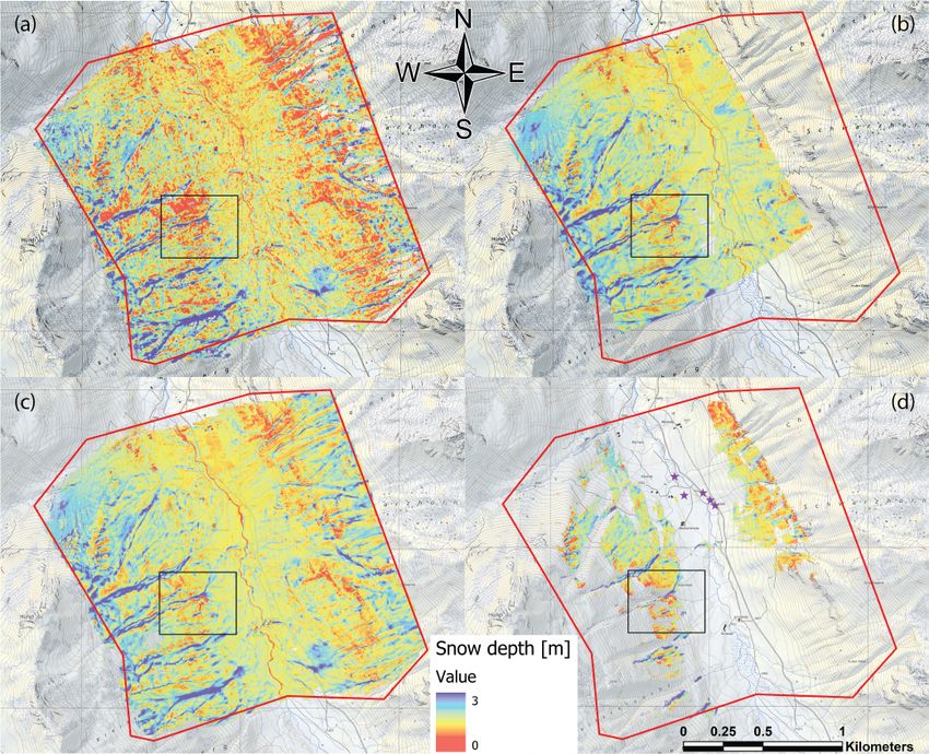
72                        L. A. Eberhard et al.: Photogrammetric platforms for spatially continuous snow depth mapping

Figure 1. Overview of the test sites: area recorded by the satellite and airplane imagery (red), area covered by the UAS imagery (blue) and
area covered by the terrestrial images (black). The purple triangles represent the location of automatic and manual snow measuring stations
around Davos. The abbreviations correspond to the snow measuring stations shown in Fig. S1. The blue star in the inset map shows the
location of the Schürlialp test site (Swiss Map Raster, source: Federal Office of Topography).

matic and multispectral bands (red–green–blue, RGB; near-               3.2   Airplane: Ultracam Eagle M3
infrared, NIR) of the Pléiades very high-resolution sensor
achieve a spatial resolution of 0.5 and 2 m, respectively.              Airborne imagery was acquired with an Ultracam Eagle M3
The 12-bit radiometric resolution of Pléiades imagery pro-              by the company Flotron on 11 April 2018 between 11:00
vides a dynamic range capable of resolving contrast in dark             and 12:00 LT. Unfortunately, the data could not be acquired
shaded areas as well as across highly reflective snow sur-              on the same day as the satellite triplet due to technical is-
faces. From 694 km above ground, the image triplet was ac-              sues on the airplane. The meteorological conditions dur-
quired along a descending orbit tracking in eastern Switzer-            ing the data acquisition were partly cloudy, and only the
land (across-track incidence angles of 17.4, 12.1 and 9.7◦ , re-        northern part of the Dischma valley was cloud free. From
spectively). Along-track incidence angles of −16.3, 7.6 and             512 images, only 242 images could be used for photogram-
17.9◦ resulted in three stereo pairs with base-over-height ra-          metric processing. Fortunately, no noticeable snowfall event
tios (B/H ) of 0.42 (images 1 and 2: pair P12), 0.19 (images 2          occurred between 6 and 11 April 2018, and the tempera-
and 3: pair P23) and 0.62 (image 1 and 3: pair P13). Although           ture was too low to allow for significant snowmelt (maxi-
both P12 and P13 have B/H recommended for photogram-                    mum 10 cm between 6 and 11 April at the low-elevation sta-
metric work (> 0.25; Astrium, 2012), P23 is below the usual             tions; see graph in Fig. S1). The Ultracam Eagle M3 features
standard to process an accurate DSM due to acute parallax               a large-format charge-coupled device (CCD) image sensor
angles. Meanwhile, larger B/H ratios, such as stereo P12,               with 450 megapixels (MP) and a pixel size of 4 µm × 4 µm
can yield unresolved areas due to terrain obstruction in steep          (see Table 1 for more information). The Ultracam Eagle M3
topography. In addition, complicated parallaxes can modify              was mounted with the 122.7 mm focal length lens and flown
the appearance of ground features and in turn challenging               at a mean altitude of 1780 m above ground level (a.g.l.), re-
stereo-matching. For this study, we processed the three stereo          sulting in a GSD of ca. 6 cm per pixel. The Ultracam Eagle
pairs and considered occlusion and accuracy of each DSM                 M3 images were recorded with a 14-bit radiometric resolu-
to create a single merged surface product, as explained in              tion. The images delivered were four-band (RGB and NIR)
Sect. 4.2.                                                              geotagged images. Furthermore, the data were delivered with
                                                                        camera positions and orientations with a DGNSS accuracy
                                                                        of 0.2 m and an inertial measurement unit (IMU) accuracy of

The Cryosphere, 15, 69–94, 2021                                                                https://doi.org/10.5194/tc-15-69-2021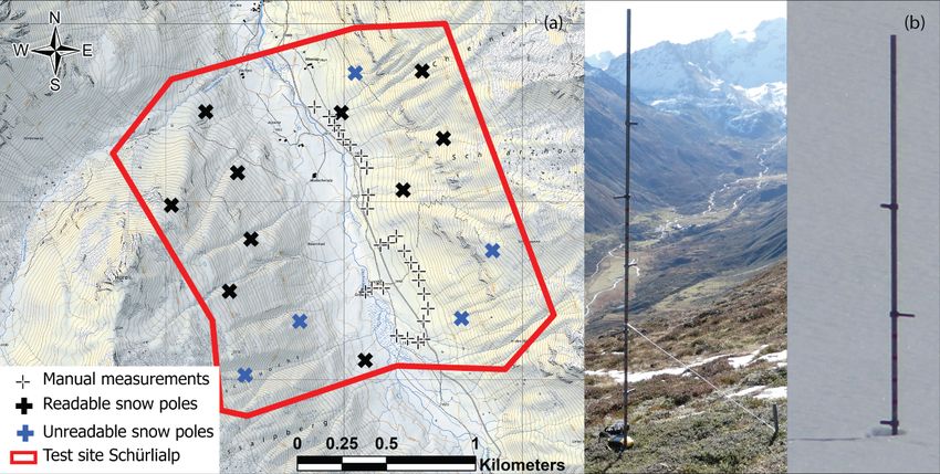
L. A. Eberhard et al.: Photogrammetric platforms for spatially continuous snow depth mapping                                     73

0.01◦ (omega, phi, kappa) and corrected for lever arm and         tion in JPEG format, covering the slopes of the northern part
boresight calibration.                                            of the Schürlialp test site (see Fig. 1).

3.3   UAS: eBee+ RTK with SenseFly S.O.D.A. camera                3.5   Reference datasets

UAS imagery of the Schürlialp area was collected on               Manual snow depth measurements and fixed snow depth
7 April 2018 at 09:27 LT for 1.5 h (three flights) with an        poles
eBee+ RTK of SenseFly equipped with the S.O.D.A. cam-
                                                                  Manual snow-probing measurements at 27 locations at the
era. This imaging payload features a 1 in. complementary
                                                                  Schürlialp test site were performed on 6 April (17 measure-
metal–oxide–semiconductor (CMOS) sensor with 20 MP
                                                                  ments) and 7 April 2018 (10 measurements). The automatic
(see Table 1 for more information) built specifically for pho-
                                                                  stations around Davos (Fig. 1) measured a decrease in snow
togrammetric applications. The images were recorded in the
                                                                  depth of 0.04 m between these 2 d at the lowest-elevation
JPEG format with 8-bit radiometric resolution for each chan-
                                                                  station Davos Flüelastrasse (5DF; 1560 m a.s.l.). For each
nel. Flying at 182 m a.g.l. on average with lateral and forward
                                                                  snow probing location, the snow depth was measured plumb
overlaps of 70 % and 60 %, respectively, yields 1550 im-
                                                                  with an avalanche probe at each corner and in the middle
ages with an average GSD of 0.04 m. A characterizing fea-
                                                                  of a 1 × 1 m square. The position of the square centre was
ture of the eBee+ RTK is the onboard DGNSS, which mea-
                                                                  recorded with a DGNSS (Trimble Geo XH 6000). As man-
sured the camera positions with a mean horizontal accuracy
                                                                  ual snow probe measurements are only possible in terrain
of ca. 0.02 m and mean vertical accuracy of ca. 0.03 m. For
                                                                  safe from avalanches, 15 fixed snow poles were installed
RTK operation, the eBee+ RTK was referenced directly in
                                                                  throughout the Schürlialp area in summer (see Fig. 2). The
the Swiss coordinate system LV95LN02, relative to mount
                                                                  snow depths values were read off the poles with binoculars
point VRS_GISGEOLV95LN02 of the national DGNSS net-
                                                                  or zoomed photos. The snow poles were marked every half
work.
                                                                  metre by pointer and red tape at every 0.1 m, allowing a mea-
                                                                  suring accuracy of ca. 0.05 m (see Fig. 2). We estimate this
3.4   Terrestrial: Canon EOS 750D
                                                                  uncertainty because a small depression often exists around
                                                                  the pole, and it is possible that the snow pole is slightly tilted
The terrestrial images were collected manually on a tripod
                                                                  by the snow load. At the time of the campaign, the snow
with a Canon EOS 750D SLR camera on 7 April 2018 start-
                                                                  depth could be read from 10 snow poles. The other five poles
ing at 10:37 LT for 1 h. The Canon EOS 750D is a digital
                                                                  were not visible due to a lack of contrast against the snow or
SLR camera featuring an APS-C CMOS sensor with 24.2 MP
                                                                  avalanches that bent them previously.
resolution. We used a zoom lens (18–55 mm) and set the fo-
cal length at 43 mm. We chose the focal length of 43 mm as a      3.6   Summer reference datasets
compromise to achieve a mean GSD in the range of the other
platforms for the selected camera locations. To ensure sta-       Mapping snow depth requires an accurate snow-free refer-
ble recording conditions, a tripod was used to take pictures      ence surface. For this study two completely snow-free sum-
from five different vantage points. The tripod was placed at      mer DSMs were considered. For the snow depth maps of
each location, and the camera was rotated on the tripod head.     the Schürlialp test site, a UAS (eBee+ RTK) flight was per-
The entire set-up was moved in one piece so that the focal        formed on 27 June 2018, yielding a final DSM with spatial
length stayed fixed. To document the camera location, the         resolution of 0.09 m. For further information about the pro-
DGNSS (Trimble Geo XH 6000) was placed on the top of              cessing workflow see Sect. 4.4. For producing snow depth
the camera, and this position was measured with a horizon-        maps extending beyond the Schürlialp test site, a DSM with
tal and vertical accuracy of 0.1 m. The GSD of this terrestrial   a spatial resolution of 0.5 m derived from an airborne laser
recording changes strongly across the slope, which affects        scan (ALS) of the Dischma valley was used. The flight cov-
the photogrammetric results. In order to achieve accurate         ered the Dischma valley but not the entire area captured by
measurement in all directions, the ray intersection angle is      the satellite and airplane imagery. The ALS flight was con-
optimal around 90 to 100◦ , which requires a sufficient B/H       ducted on 5 and 6 August 2015 by Milan Geoservice GmbH
ratio (Luhmann et al., 2014, p. 547), while also promoting        with a Riegl LMS-Q 780 scanner. Milan Geoservice GmbH
terrain occlusions, making terrestrial recording challenging.     delivered an oriented, unclassified point cloud in the refer-
With the camera positioned at the bottom of the Dischma val-      ence system LV03 LN02. Ground point classification and
ley, some slopes to the south-west and to the north-east are      DSM generation were done using the software LAStools
more than 1 km away. Thus, the GSD varies between 0.01 m          (Isenburg, 2014).
per pixel and 0.1 m per pixel with a mean GSD of 0.05 m per
pixel. Towards the north and south sides, the flat valley floor
is not suitable for snow depth mapping. A total of 268 images
were recorded on 7 April 2018 with 8-bit radiometric resolu-

https://doi.org/10.5194/tc-15-69-2021                                                         The Cryosphere, 15, 69–94, 2021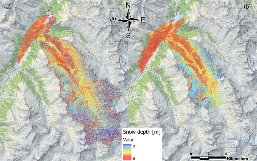
74                                                  L. A. Eberhard et al.: Photogrammetric platforms for spatially continuous snow depth mapping

Table 1. Summary of the photographic data collection with the satellite, airplane, UAS and terrestrial platforms.

                                                         Satellite: Pléiades         Airplane: Ultracam Ea-   UAS: eBee+ RTK with      Terrestrial: Canon EOS
                                                                                     gle M3                   SODA camera              750D
                             Sensor type                 Pushbroom scanner           CCD image sensor         1 in. CMOS sensor        APS-C CMOS sensor
                                                         TMA optics
                             Sensor resolution           Panchromatic       array    450 MP                   20 MP                    24.2 MP
                                                         assembly:      5 × 6000
                                                         (30 000     cross-track)
                                                         pixels; multispectral ar-
                                                         ray assembly: 5 × 1500
    Platform information

                                                         (7500 in cross-track)
                                                         pixels
                             Focal length                12.905 m                    122.7 mm                 10.6 mm                  43 mm
                             Pixel size                  13 µm × 13 µm         in    4 × 4 µm                 2.4 × 2.4 µm             3.7 × 3.7 µm
                                                         panchromatic band
                             Sensor dimensions           390 mm × 3 mm               105.85 × 68.03 mm        13.2 × 8.8 mm            22.3 × 14.9 mm
                             Radiometric resolution      12-bit                      14-bit                   8-bit                    8-bit
                             Image type                  Multispectral TIFF and      High-resolution multi-   sRGB JPEG                sRGB JPEG
                                                         panchromatic TIFF           channel RGBI TIFF
                             Acquisition date            7 April 2018                11 April 2018            7 April 2018             7 April 2018
                             Start of acquisition        10:17 LT                    11:05 LT                 09:27 LT                 10:37 LT
                             Number of pictures          3                           521 (242 cloud free)     1550                     268
                             Area covered                140 km2                     75.7 km2                 3.59 km2                 1.12 km2
    Acquisition details

                             Mean flight height          694 km a.g.l.               1780 m a.g.l.            181 m a.g.l.             Mean distance from the
                                                                                                                                       target: 1 km
                             Mean GSD                    0.7 m per pixel (resam-     0.06 m per pixel         0.04 m per pixel         0.05 m per pixel
                                                         pled to 0.5 m per pixel)
                                                         for the panchromatic
                                                         band (nadir); 2.8 m per
                                                         pixel (resampled to 2 m
                                                         per pixel) for the multi-
                                                         spectral bands (nadir)

4                          Data processing                                                       More specific aspects of data processing and performance
                                                                                                 evaluation are provided in the following sections.
Before a photogrammetric snow depth map or an orthoimage
can be generated, a DSM must first be produced from the im-
                                                                                                 4.1    Coordinate systems
ages of each platform. We used the software packages Ag-
isoft Metashape version 1.5.3/1.5.5 (for airplane, UAS and
terrestrial data) and a combination of ERDAS Imagine 2018,                                       Analysing data in the same horizontal coordinate system with
Ames Stereo Pipeline (ASP 2.6.2) and GDAL (GDAL/OGR                                              the same vertical datum is fundamental for the calculation of
contributors, 2020) (for satellite data) for photogrammetric                                     snow depth maps. This requires documentation and verifi-
triangulation, restitution of DSM and production of orthoim-                                     cation of the coordinate systems and vertical datums used
ages. Once DSMs and orthoimages were created as raster                                           across the processing workflow for each dataset. For ex-
datasets, snow depth maps were calculated using ArcGIS Pro                                       ample, the geometry of the satellite imagery is defined in
version 2.4.2 by subtracting the summer DSM from the win-                                        terms of a WGS84 ellipsoid, both for planimetry and el-
ter DSM. The resulting snow depth maps were validated and                                        evation (height above ellipsoid, HAE). Other data such as
compared using two different strategies in order to evaluate                                     the summer ALS DSM were delivered in the Swiss coordi-
the performance of the individual platforms and workflows.                                       nate system LV03/LN02. All DGNSS data (GCP, UAS) were

The Cryosphere, 15, 69–94, 2021                                                                                         https://doi.org/10.5194/tc-15-69-2021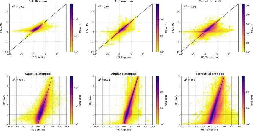
L. A. Eberhard et al.: Photogrammetric platforms for spatially continuous snow depth mapping                                            75

Figure 2. Panel (a) shows the distribution of the snow poles and the manual snow measurements at the Schürlialp test site. The snow poles
are separated into the readable (black crosses) and unreadable ones (blue crosses). The thin black crosses show the locations of the manual
measurements. The two images in (b) show a snow pole in summer and winter. The snow poles have a hinge at the foot and are tensioned
back with a nylon cord. This way they simply fold down in the event of an avalanche and are not dragged along (Swiss Map Raster, source:
Federal Office of Topography).

recorded in RTK mode based on a swipos-GIS/GEO correc-                  DSM postprocessing and production of orthoimagery with
tion stream using the LN02 height system.                               custom scripts in GDAL 2.4.1. Satellite image triplet bundle
   Because the conversion from ellipsoidal heights (WGS84)              block triangulation (BBA) is best performed on WGS84 to
to LN02 is only achieved by means of interpolation, we de-              ensure unambiguous rational polynomial coefficient (RPC)
fined the new Swiss height system LHN95 and the local ref-              modelling. The 14 GCPs from the field survey (see Sect. 3)
erence system LV95 as the main reference frame for this                 with coordinates accurate to the decimetre on LV95 and
study. The height system LHN95 (Landeshöhennetz, 1995)                  Bessel HAE were converted with REFRAME to UTM32N
is derived from geopotential number and provides rigorous               (ETRS89) and WGS84 HAE. BBA triangulation was com-
orthometric heights with consideration of the Alpine uplift             pleted on the 0.5 m resolution panchromatic images with
(Schlatter and Marti, 2005). However, because of its official           manual input and manual refinements of the 14 GCPs and
and legal status, most of the data in Switzerland are mea-              32 tie points to achieve a robust BBA solution. Final quality
sured in the LN02 height system. Therefore, the datasets                assessment of the triangulation was derived from leave-one-
were provided either on LN02 or on WGS84, and all con-                  out cross-validation (LOOCV) (Sirguey and Cullen, 2014),
versions from LN02 to LHN95 and WGS84 to LHN95 were                     whereby each GCP is set as a checkpoint in turn to gener-
handled using the REFRAME library provided by swisstopo.                ate an independent residual, yielding 0.43 m CE90 (circular
REFRAME was used to create conversion grids to accom-                   error of 90 %) and 0.43 m LE90 (linear error of 90 %).
modate (i) WGS84 to Bessel ellipsoidal height separation                   Dense stereo-matching at full resolution (0.5 m) was com-
(deterministic calculation), (ii) Bessel to LHN95 separation            pleted with ASP using a hybrid global-matching approach
(CHGEO2004 geoid model) and (iii) LHN95 to LN02 sepa-                   (Hirschmuller, 2008; d’Angelo, 2016; Beyer et al., 2018).
ration (HTRANS).                                                        DSMs were produced from a point cloud at 2 m resolution on
                                                                        UTM32N/WGS84, reprojected to LV95 with GDAL (cubic
4.2   Satellite data-processing workflow                                convolution) and height-adjusted to LHN95 using conversion
                                                                        grids mentioned in Sect. 4.1. Maps of ray intersection errors
Processing of Pléiades satellite images involved triangulation          from stereo-matching with ASP measure the minimal dis-
in ERDAS Imagine 2018, surface restitution in NASA Ames                 tance between rays for pairwise stereo and are indicative of
Stereo Pipeline (ASP; Shean et al., 2016; Beyer et al., 2018)           the quality of the match. In tri-stereo configuration, we gener-
version 2.6.2 (https://doi.org/10.5281/zenodo.3247734), and             ated a DSM and map of ray intersection error for each stereo

https://doi.org/10.5194/tc-15-69-2021                                                               The Cryosphere, 15, 69–94, 2021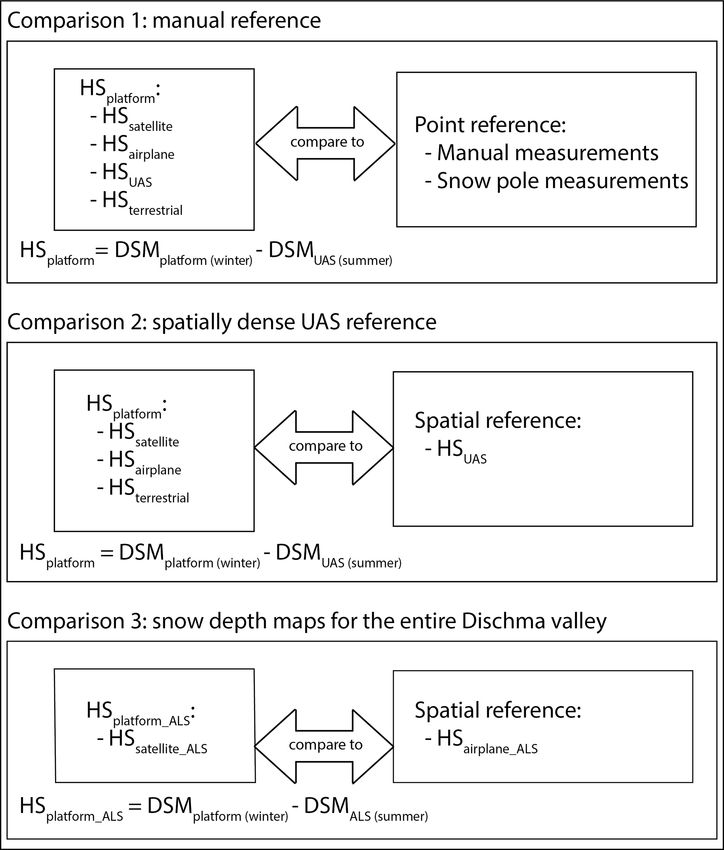
76                       L. A. Eberhard et al.: Photogrammetric platforms for spatially continuous snow depth mapping

pair. We blended DSMs with GDAL using a weighted arith-             (cx, cy, b1, b2, k1, k2, k3, k4, p1, p2; see Agisoft LLC, 2019
metic mean, whereby the elevation from each constituent             for more information about the frame camera model) were
DSM was weighted by its corresponding ray intersection er-          fixed to 0 according to the calibration report of the camera. To
ror. A map of standard error in the weighted mean was gen-          improve the geolocation accuracy after alignment, 29 GCPs
erated by uncertainty propagation. The relatively small B/H         distributed over the Dischma valley were imported into Ag-
ratio of the pair P23 resulted in significantly higher noise that   isoft. A total of 15 CPs were used to control the geolocation
compromised the tri-stereo blending. Alternatively, blending        accuracy (see Sect. 3 for more information about GCP and
only DSM members P12 and P13 provided a better surface,             CP). The CPs resulted in an RMSE value of 0.14 m for the
with noise comparable to or better than the bi-stereo with          XY coordinates and an RMSE value of 0.19 m for the Z.
the largest B/H ratio (P13). P23 was only used to fill gaps         After alignment and refinement of the geolocation accuracy,
remaining from the two-member blending. The final DSM               the dense point cloud was produced with the depth filter-
was used to orthorectify each of the three images, and the          ing method “aggressive”. The filtering method “aggressive”
three pan-sharpened orthoimages were then blended together          gives, in our experience, the best results for snow-covered
to create a single final orthoimage. Finally, the map of stan-      surfaces and filters out most outliers, leading to cleaner sur-
dard error for the blended DSM was used to set all cells of the     face models. The DSM was generated from the dense point
DSM to no data where the ray intersection error was greater         cloud at a 0.11 m per pixel resolution without interpolating
than 1 panchromatic pixel (0.5 m) as larger errors were found       voids. Finally, an orthoimage at a resolution of 0.5 m per
to often be indicative of erroneous stereo-matching.                pixel was created based on the DSM.
    Despite the robust survey quality indicated by LOOCV, a
remaining 27.5 arcsec tilt (66.7 ppm, or ±1 m over 15 km)           4.4   UAS-processing workflow
along the north-west–south-east axis of the imagery was de-
tected in the blended DSM after differencing with the sum-          The eBee+ RTK has an IMU on board for flight control for
mer ALS DSM. To correct the tilt, points were manually              which the accuracy and calibration are not given by the man-
placed along snow-free roads in the imagery, and spot el-           ufacturer. Therefore, we have processed the imagery in Ag-
evations were extracted from the blended DSM and ALS                isoft Metashape without IMU but with the DGNSS data only.
surfaces. The distribution of offsets along roads in the city       Since the mount point applied the corrections for the Swiss
and inside the valley revealed enough linearity to justify the      coordinate system LV95 LN02 during the flight, the camera
fitting of a plane in 3D space. This hyperplane was fit via         positions of the eBee+ RTK had to be transformed into the
least squares through the residuals to create a corrective grid     vertical coordinate system LHN95 before processing could
covering the imagery footprint which was used to adjust the         take place. This was done by first exporting the camera po-
blended DSM.                                                        sition of the eBee+ RTK images stored in EXIF metadata to
                                                                    a text file used as input for REFRAME to convert the posi-
4.3   Airplane data-processing workflow                             tions into LHN95 for use in Agisoft Metashape. Again, the
                                                                    use of the CHGeo2004 geoid model in Agisoft Metashape al-
The Ultracam Eagle M3 images are distinguished by a high            lowed for consistent processing in the vertical height system
dynamic range (14-bit radiometric resolution). We used Ag-          LHN95. The images were then aligned and georeferenced
isoft Metashape for image processing, which can be applied          without GCPs and using only CPs to assess the accuracy of
for images acquired with RGB- or multispectral-type frame           the triangulation. SenseFly, the manufacturer of the eBee+
sensors (Westoby et al., 2012) and supports up to 16-bit            RTK, claims that this approach of integrated sensor orien-
radiometric resolution. Since the southern part of the Dis-         tation (ISO) can achieve accuracies of the order of 0.03 m
chma valley was cloud-covered, the images were manually             horizontally and 0.05 m vertically (level of accuracy of 1 to
sorted into cloud-free and cloud-covered images. The cam-           3× GSD) (Benassi et al., 2017; Roze et al., 2017). Benassi
era positions delivered in the height system LN02 were con-         et al. (2017) showed an RMSE value of 0.02 to 0.03 m for
verted into LHN95 with REFRAME for input into Agisoft               the horizonal coordinates of checkpoints and an RMSE value
Metashape. The use of the CHGeo2004 geoid model in Ag-              of 0.02 to 0.1 m for the vertical coordinates of CPs for a
isoft Metashape then allows for consistent processing in the        flight with RTK solution but without GCPs. We assessed the
vertical height system LHN95.                                       model accuracy using six of the signalled CPs at the Schür-
   The images were imported into Agisoft Metashape and              lialp test site, resulting in total RMSE values for XY and
aligned. The Ultracam Eagle M3 is a professional pho-               Z coordinates of 0.05 and 0.1 m, respectively. A dense point
togrammetric camera that has been accurately calibrated by          cloud was produced with the filtering mode “aggressive”. Fi-
the vendor so that a refinement of the internal camera param-       nally, the DSM was created with a resolution of 0.09 m per
eters by Agisoft is not desirable. Therefore before alignment,      pixel without interpolation, which was used to produce an
the camera parameters were fixed in Agisoft Metashape to            orthoimage at 0.04 m per pixel.
a focal length of 122.7 mm and 0.004 mm × 0.004 mm pixel               The summer eBee+ RTK flight was processed with the
sizes (see Table 1). All the other camera model parameters          same workflow as the winter eBee+ RTK flight. This re-

The Cryosphere, 15, 69–94, 2021                                                           https://doi.org/10.5194/tc-15-69-2021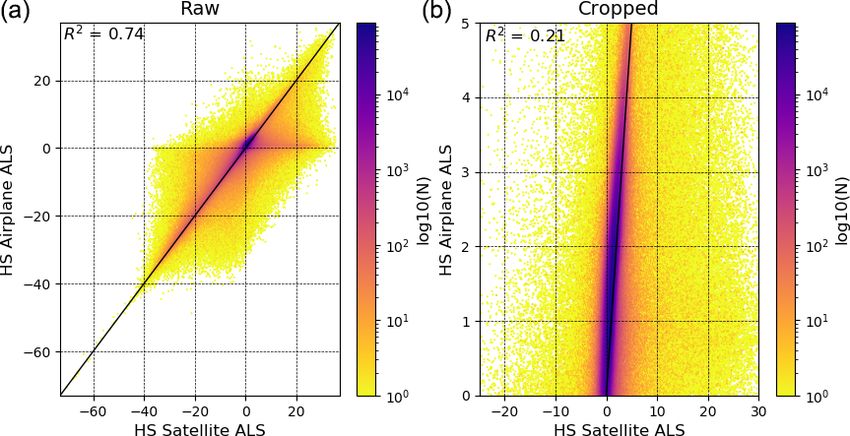
L. A. Eberhard et al.: Photogrammetric platforms for spatially continuous snow depth mapping                                     77

sulted in a DSM with a resolution of 0.09 m per pixel and         4.6.1   Comparison 1: manual reference
an orthoimage of 0.04 m per pixel. Six CP markers were sig-
nalled on the ground for the summer eBee+ RTK survey and          For comparison 1 only the Schürlialp (3.59 km2 ) test site
measured with a Stonex S800 receiver and S4II Win Mo-             was considered. This provided a detailed comparison of each
bile 6.5 controller providing accuracy for the horizontal po-     platform’s accuracy against the manual measurements and
sition between 0.014 to 0.022 m and a vertical position ac-       the snow pole measurements. The snow depth maps are cal-
curacy of 0.02 m. Photogrammetric modelling in Agisoft re-        culated with the UAS summer DSM of 27 June 2018. To
sulted in RMSE values for the XY and Z of 0.02 and 0.05 m,        keep interpolation errors as low as possible, the winter DSMs
respectively.                                                     were exported at their highest native spatial resolution: satel-
                                                                  lite DSM at 2 m, airplane DSM at 0.11 m, UAS DSM at
4.5   Terrestrial-processing workflow                             0.09 m and terrestrial DSM at 0.11 m resolution. Prior to gen-
                                                                  erating the snow depth maps, the summer and winter DSMs
                                                                  were made coincident (equal size and winter DSM snapped
Terrestrial snow depth mapping is a compromise between
                                                                  to summer DSM). The summer DSM was then subtracted
measurement requirements and time. Therefore, due to the
                                                                  from the winter DSM, resulting in the corresponding plat-
avalanche situation and the logistical effort that would have
                                                                  form snow depth map. Finally, to compare the snow depth
been necessary, no control points could be distributed over
                                                                  maps from each platform with the manual reference measure-
the area during data capture. The GCPs and CPs used for
                                                                  ments, a buffer with a radius of 0.7 m (i.e. the half-diagonal
the satellite, airplane and UAS are not visible in the terres-
                                                                  of the 1 m × 1 m sample square) was created from the centre
trial images. Only the camera positions were measured with
                                                                  position of the manual measurement. For each snow depth
a DGNSS (see Sect. 3.4) during recording. However, this
                                                                  map, the mean value and the standard deviation were calcu-
did not allow us to determine the precise offset between the
                                                                  lated within this buffer area. Because the selected buffer has
DGNSS antenna phase and the principal point of the cam-
                                                                  a smaller area than the resolution of the satellite data, the cell
era. For this reason, the measurement accuracy of the camera
                                                                  value was extracted at the position of the snow depth mea-
position used in Agisoft Metashape was set to 0.2 m.
                                                                  surements and the snow poles for this data. In Sect. 4.6.4
   To refine the georeferencing of the terrestrial images, fea-
                                                                  further details of the accuracy and precision measures calcu-
tures such as stones, bushes and house corners emerging
                                                                  lated are defined.
from the snow were detected manually on the terrestrial im-
ages to serve as GCPs. The features of nine GCPs were then
                                                                  4.6.2   Comparison 2: spatially dense UAS reference
identified on the orthoimage and DSM products from the
UAS summer survey from which coordinates were extracted.
                                                                  The high accuracy of UAS data for snow depth mapping has
The images were therefore sorted into the five camera sta-
                                                                  been successfully tested in various studies (Vander Jagt et al.,
tions in Agisoft Metashape and aligned and georeferenced
                                                                  2015; Bühler et al., 2016; De Michele et al., 2016; Harder et
with GCPs. Again, the dense point cloud was created with
                                                                  al., 2016; Cimoli et al., 2017; Redpath et al., 2018; Avanzi et
the “aggressive” filter and a DSM and orthoimage produced
                                                                  al., 2018; Eker et al., 2019). With comparison 2, we compare
at 0.11 and 0.06 m per pixel, respectively.
                                                                  the spatially continuous snow depth map of the UAS with the
                                                                  snow depth maps of the other three platforms. Therefore, the
4.6   Snow depth map validation and comparison                    winter and summer DSMs of the UAS were exported from
      strategies                                                  Agisoft Metashape at a spatial resolution of 0.11 m (for ter-
                                                                  restrial and airplane comparison) and 2 m (for satellite com-
Three comparison strategies were developed to compare the         parison). These DSMs were then aligned to the snow depth
photogrammetric data and investigate the performance of           maps used in the comparison via cubic-convolution resam-
the different platforms (see Fig. 3). Comparison 1 aims to        pling. Finally, the winter DSMs were subtracted from the
validate the snow depth maps for the Schürlialp test site         summer DSMs, resulting in three snow depth maps, with
using the manual and snow pole measurements (described            that from the UAS used as reference for comparison 2. With
in Sect. 4.6.1). Comparison 2 compares the different snow         these snow depth maps, the metrics and plots described in
depth maps with the spatially dense UAS snow depth map            Sect. 4.6.4 were calculated.
used as spatial reference (described in Sect. 4.6.2). The UAS
summer reference is used for calculating the snow depth           4.6.3   Comparison 3: snow depth maps of the entire
maps of comparison 1 and comparison 2. Finally, in com-                   Dischma valley
parison 3, snow depth maps of satellite and airplane imagery
are calculated and compared with the ALS summer scan (de-         The summer ALS scan covers a much larger area (100 km2 )
scribed in Sect. 4.6.3) to show the potential of measuring        compared with the UAS summer flight. We calculated the
snow depth distribution over larger areas. Section 4.6.4 de-      snow depth maps from the satellite and the airplane imagery
scribes the accuracy measures used within this paper.             using the summer ALS scan. We re-exported the airplane

https://doi.org/10.5194/tc-15-69-2021                                                         The Cryosphere, 15, 69–94, 2021
78 L. A. Eberhard et al.: Photogrammetric platforms for spatially continuous snow depth mapping
Figure 3. Flow chart illustrating the three comparison strategies. With HSplatform we refer to the snow depth map of the respective platform.
HSplatform_ALS is the snow depth map of the respective platform calculated with the ALS summer DSM.
DSM at 2 m resolution with Agisoft Metashape. We aligned sure of accuracy. The standard deviation (SD) is a common
the satellite and the airplane DSM to the ALS DSM and sub- measure of precision and measures the dispersion of the data
tracted the summer ALS DSM from each winter DSM with in relation to the mean (Maune and Naygandhi, 2018). To
cubic-convolution resampling. To compare snow depth mea- detect systematic vertical offsets of the snow depth maps,
surements over a much larger area, we used the airplane snow the mean bias error (MBE) and the median of the bias er-
depth map as a reference to calculate the accuracy and preci- rors (MdBE) were calculated. The MdBE is less sensitive to
sion of the satellite map. outliers than the MBE, and the difference between the two
measures gives an indication of the role of outliers in the met-
4.6.4 Accuracy and precision measures rics. Similarly, the NMAD is a measure of precision that is
more robust to outliers than SD (Höhle and Höhle, 2009).
We evaluated the snow depth maps in the different compar- Box plots and normalized histograms were calculated for
isons using a selection of accuracy and precision measures the first two comparison strategies to illustrate the accuracy
(see Table 3). Accuracy defines how close an estimated value assessment by graphical means. The box plot summarizes
is to a standard or accepted value of a given quantity. Preci- the statistical measures of the median, quantile, span and in-
sion (dispersion) on the other hand describes how close mea- terquantile distance that support a graphical interpretation of
surements agree with each other despite possible systematic the results. For the histogram the values were normalized,
bias. The root mean square error (RMSE) is a common mea-
The Cryosphere, 15, 69–94, 2021 https://doi.org/10.5194/tc-15-69-2021L. A. Eberhard et al.: Photogrammetric platforms for spatially continuous snow depth mapping 79
and the y axis shows the relative frequency of the values. nus alnobetula) can influence the snow depth when using a
We considered a filtered version of the errors in each plat- DSM as summer reference.
form comparison, whereby errors greater than 2 SDs were The satellite snow depths have the largest dispersion
classified as outliers and removed. There are different meth- (SD = 0.77 m and NMAD = 0.43 m) in comparison to the
ods described in the literature to remove outliers; one is to manual and snow pole measurements. The box plots and
remove data in excess of 3 SDs (Höhle and Höhle, 2009; the histograms (Fig. 7) illustrate the dispersion. The negative
Novac, 2018). We prefer to be more liberal and filtered the MBE (−0.46 m) and negative MdBE (−0.40 m) suggest that
data only with a threshold of 2 SDs, where, for normal dis- the satellite snow depth map is systematically lower com-
tribution, 95 % of the values would be found. The accuracy pared to the manual and fixed snow pole measurements. Af-
and precision measures as well as the box plot and histogram ter filtering the raw data, the satellite RMSE value is 0.52 m,
were calculated again with the filtered data. Additionally, we and the SD is 0.39 m. This improvement can be partially ex-
generated scatter plots for comparison 2 and comparison 3 to plained by a single large outlier (1H = −4.47 m) removed
illustrate the dispersion in snow depth from satellite, airplane with the filter. The satellite snow depth map, however, re-
and terrestrial platforms compared to the reference from the mains negatively biased at the location of manual and snow
UAS platform and calculated the Pearson correlation coeffi- pole measurements.
cient (R 2 ). To analyse only the per-pixel value correlation of The airplane returns an RMSE value of 0.20 m and the
the snow depth maps in the positive realistic range, we calcu- UAS an RMSE value of 0.21 m. Only 27 out of 37 mea-
late a second scatter plot, where all negative values and val- surements could be considered for the airplane. The SDs of
ues higher than a maximum snow depth (5 m defined by ex- the airplane and the UAS are the same (SD = 0.20 m). The
pert opinion and based on the snow depth distribution) of the NMAD (0.17 m) of the airplane is 0.03 m higher than the one
reference snow depth map are deleted, and the Pearson cor- of the UAS (0.14 m), but again the difference is small. The
relation coefficient (R 2 ) is calculated again. This gives us an box plot and the histogram illustrate greater dispersion of the
indication of how the snow depth maps correlate in the posi- errors in the airplane despite the small differences in the ac-
tive and most relevant range for most modelling purposes. curacy and precision measures compared to the UAS. The
MBE (0.03 m) of the airplane is slightly positive, but MdBE
(−0.03 m) is negative by the same value. Therefore, we con-
sider this difference of 0.06 m negligible and assume that the
5 Results airplane snow depth map is not biased. This result is also
supported by the box plot for both raw and filtered data. By
The satellite imagery covered 140 km2 , the airplane imagery applying the threshold for outliers, RMSE, SD and NMAD
covered 75.7 km2 in the northern part of the Dischma val- are found to be equal at 0.17 m for the airplane and slightly
ley, the UAS imagery covered 3.59 km2 around Schürlialp, better (0.11 to 0.16 m) for the UAS. The MBE (−0.07 m) and
and finally the terrestrial images covered the smallest area of MdBE (−0.07 m) indicate that the UAS snow depth map has
1.12 km2 . The orthoimages in Fig. 4 show the footprint cov- a slight negative bias. This is again consistent with Bühler
ered by each platform. The orthoimages of both the satellite et al. (2016), who found a slight underestimation of snow
and UAS are cloud-free, while the orthoimage of the airplane depth for UAS. Normally it should be the same for the air-
only covers the northern part of the Dischma valley because plane, but this can be due to the difference in processing as
of clouds. The orthoimage of the terrestrial imagery reveals the airplane was processed with GCPs and the UAS without.
the suboptimal recording geometry and large terrain occlu- However, box plots, histograms and accuracy measures of
sions. filtered versions of the snow depth maps show that the UAS
The following subsections present the results in detail ac- has the best accuracy compared to manual reference mea-
cording to the comparison strategies described in Sect. 4.6. surement. For the terrestrial snow depth map, only four snow
Section 5.1 shows the results of comparison 1. Section 5.2 pole measurements could be considered, and therefore the
continues with the results of comparison 2. Finally, in statistical statements are not meaningful. For completeness
Sect. 5.3 the snow depth maps of the entire Dischma valley they are nevertheless listed in Table 4.
are illustrated.
5.2 Results of comparison 2: spatially dense UAS
5.1 Results of comparison 1: manual reference reference
Using the workflows described in the Sect. 4.6.1, a snow Accurate and spatially distributed calculation of snow depth
depth map was calculated for each platform. The snow depth in alpine terrain from UAS imagery has been well docu-
maps are shown in Fig. 5 and a zoomed inset in Fig. 6. All mented in recent publications (e.g. Vander Jagt et al., 2015;
four maps show similar snow depth distribution patterns, in- Bühler et al., 2016; De Michele et al., 2016; Harder et al.,
cluding characteristic snow features such as wind deposits. 2016; Cimoli et al., 2017; Redpath et al., 2018; Avanzi et
Figure 6 illustrates how vegetation (here the bush species Al- al., 2018; Eker et al., 2019) and supported by our results.
https://doi.org/10.5194/tc-15-69-2021 The Cryosphere, 15, 69–94, 202180 L. A. Eberhard et al.: Photogrammetric platforms for spatially continuous snow depth mapping Figure 4. (a) Orthoimage of the satellite data, (b) orthoimage of the airplane data. The area recorded by the airplane is theoretically larger than the area recorded by the satellites, but due to the clouds only part of the images could be used for producing DSM and orthoimagery. (c) The orthoimage of the UAS data and (d) orthoimage of the terrestrial data. The red polygon in (a), (b), (c) and (d) indicates the Schürlialp site test. The violet stars in (d) indicate the five camera positions of the terrestrial recordings (Swiss Map Raster, source: Federal Office of Topography; Pléiades data© CNES 2018, Distribution Airbus DS). Comparison 1 confirmed that with an RMSE value of 0.16 m are also mainly located at the valley floor, the accuracy analy- and an NMAD value of 0.11m for the filtered data, the UAS sis of comparison 1 may not fully capture the true accuracy of snow depth map is within the expected accuracy for process- the snow depth products. Therefore, comparison 2 allow us to ing with ISO and without GCP. However, due to the rather more comprehensively analyse the performance of satellite, low number of manual and snow pole measurements, which airplane and terrestrial snow depth maps against the entire The Cryosphere, 15, 69–94, 2021 https://doi.org/10.5194/tc-15-69-2021
L. A. Eberhard et al.: Photogrammetric platforms for spatially continuous snow depth mapping                                                81

Table 2. Description of the summer datasets used for the calculation of the snow depth maps.

                                                                    UAS: eBee+ RTK     ALS: LMS-Q 780
                                               Acquisition date     27 June 2018       5–6 August 2015
                         Acquisition details   Number of pictures   1449               –
                                               Covered area         3.66 km2           100 km2
                                               Mean flight height   184 m a.g.l.       2330 m a.g.l.
                                               Point density        155 points m−2     11.8 points m−2 (after postprocessing)
                                               GSD                  0.04 m per pixel   –
                                               Resolution DSM       0.09 m per pixel   0.5 m per pixel

Figure 5. Snow depth maps of the Schürlialp test site from the satellite (a), the airplane (b), the UAS (c) and the terrestrial data (d). On
the terrestrial snow depth map, the camera positions are indicated with violet stars. The red polygon depicts the extent of the Schürlialp
test site. The black box indicates the zoomed inset shown in Fig. 6 (Swiss Map Raster, source: Federal Office of Topography; Pléiades data
© CNES 2018, Distribution Airbus DS).

https://doi.org/10.5194/tc-15-69-2021                                                                           The Cryosphere, 15, 69–94, 2021
82 L. A. Eberhard et al.: Photogrammetric platforms for spatially continuous snow depth mapping Figure 6. Inset of the Schürlialp snow depth maps shown in Fig. 5, with the scale ranging from −3 to 3 m to illustrate the negative snow depths caused by the vegetation. The effect of bushes (species Alnus alnobetula) under compression by the snow is visible as the greatest negative snow depth values (dark red) in (a) satellite, (b) airplane, (c) UAS and (d) terrestrial snow depth map draped over the swisstopo basemap. An orthoimage for the same extent is shown in (e) from the UAS summer flight and shows a hillshade of the summer ALS scan. Positive snow depth values reach up to 5 m in the gulley features in the study site (Swiss Map Raster, source: Federal Office of Topography; Pléiades data © CNES 2018, Distribution Airbus DS). The Cryosphere, 15, 69–94, 2021 https://doi.org/10.5194/tc-15-69-2021
L. A. Eberhard et al.: Photogrammetric platforms for spatially continuous snow depth mapping                                                83

Table 3. Accuracy and precision measures adapted from Höhle and Höhle (2009).

                      1HSj : error in the snow depth at location j
                      HSref                                                1HSj = HSmodel − HSref
                        j : reference snow depth at location j                      j         j
                      HSmodel
                        j     : model snow depth at location j
                                                                                         s
                                                                                                 n
                      Root mean square error (RMSE)                        RMSE =            1 P 1HS2
                                                                                             n      j
                                                                                               j =1
                                                                                   n
                                                                           µ̂ = n1
                                                                                   P
                      Mean bias error (MBE)                                          1HSj
                                                                                      j =1
                                                                                  s
                                                                                              n
                      Standard deviation (SD)                              σ̂ =         1    P
                                                                                                 (1HSj − µ̂)2
                                                                                      (n−1)
                                                                                            j =1

                      Median of the bias errors (MdBE; 50 % quantile)      mBE = median (1HS)
                      Normalized median absolute deviation (NMAD)          NMAD = 1.4826 · median( 1HSj − mBE )
                      Threshold for classifying outliers                    1HSj > 2 · σ̂

Figure 7. Box plots with single-value plots for comparison 1. The orange line depicts the median, the star the mean bias error (MBE). The
25th and 75th quartiles are represented by the boxes and the 5th and 95th percentiles by the whiskers. The left box plot shows the raw data
and the right box plot the data where plus or minus 2 SDs are removed. Because of the small sample size of the terrestrial data, applying
such a threshold does not have statistical relevance, and therefore the terrestrial data are not shown in the right box plot anymore. To better
illustrate the distribution of the error, we calculated single-value plots and included them into the box plots. Note the single large outlier
(−4.47 m) from the satellite data is not shown in the raw data to improve interpretation.

surface mapped by the UAS winter flight at the Schürlialp                    Again, the satellite data show the largest error dispersion
study site. The box plot (Fig. 8) shows that all three platforms          compared to the airplane and terrestrial data. The box plot
estimate snow depth within a similar range after filtering the            and histogram of the satellite data illustrate that the satellite
data. Furthermore, the normalized histograms of the raw and               snow depth map is slightly negatively biased over the Schür-
the filtered data show that the errors are normally distributed.          lialp test site (MBE = −0.21 m, MdBE = −0.19 m). After

https://doi.org/10.5194/tc-15-69-2021                                                                    The Cryosphere, 15, 69–94, 2021
You can also read