Sensitivity of Greenland ice sheet projections to spatial resolution in higher-order simulations: the Alfred Wegener Institute (AWI) contribution ...
←
→
Page content transcription
If your browser does not render page correctly, please read the page content below
The Cryosphere, 14, 3309–3327, 2020
https://doi.org/10.5194/tc-14-3309-2020
© Author(s) 2020. This work is distributed under
the Creative Commons Attribution 4.0 License.

Sensitivity of Greenland ice sheet projections to spatial resolution
in higher-order simulations: the Alfred Wegener Institute (AWI)
contribution to ISMIP6 Greenland using the Ice-sheet and Sea-level
System Model (ISSM)
Martin Rückamp1 , Heiko Goelzer2,3,4 , and Angelika Humbert1,5
1 Alfred-Wegener-Institut Helmholtz-Zentrum für Polar- und Meeresforschung, Bremerhaven, Germany
2 Institutefor Marine and Atmospheric research (IMAU), Utrecht University, Utrecht, the Netherlands
3 Laboratoire de Glaciologie, Université Libre de Bruxelles, Brussels, Belgium
4 NORCE Norwegian Research Centre, Bjerknes Centre for Climate Research, Bergen, Norway
5 Faculty of Geosciences, University of Bremen, Bremen, Germany

Correspondence: Martin Rückamp (martin.rueckamp@awi.de)

Received: 30 December 2019 – Discussion started: 14 January 2020
Revised: 13 July 2020 – Accepted: 28 July 2020 – Published: 2 October 2020

Abstract. Projections of the contribution of the Greenland        dicates a converging behaviour below a 1 km horizontal res-
ice sheet to future sea-level rise include uncertainties pri-     olution. A driving mechanism for differences is the ability
marily due to the imposed climate forcing and the initial         to resolve the bedrock topography, which highly controls ice
state of the ice sheet model. Several state-of-the-art ice flow   discharge to the ocean. Additionally, thinning and acceler-
models are currently being employed on various grid reso-         ation emerge to propagate further inland in high resolution
lutions to estimate future mass changes in the framework of       for many glaciers. A major response mechanism is sliding,
the Ice Sheet Model Intercomparison Project for CMIP6 (IS-        with an enhanced feedback on the effective normal pressure
MIP6). Here we investigate the sensitivity to grid resolution     at higher resolution leading to a larger increase in sliding
of centennial sea-level contributions from the Greenland ice      speeds under scenarios with outlet glacier retreat.
sheet and study the mechanism at play. We employ the finite-
element higher-order Ice-sheet and Sea-level System Model
(ISSM) and conduct experiments with four different horizon-
                                                                  1   Introduction
tal resolutions, namely 4, 2, 1 and 0.75 km. We run the sim-
ulation based on the ISMIP6 core climate forcing from the         Climate change is the major driver of global sea-level rise
MIROC5 global circulation model (GCM) under the high-             (SLR), which has been shown to be accelerating (Nerem
emission Representative Concentration Pathway (RCP) 8.5           et al., 2018; Shepherd et al., 2019). The Greenland ice sheet
scenario and consider both atmospheric and oceanic forcing        (GrIS) has contributed to about 20 % of sea-level rise during
in full and separate scenarios. Under the full scenarios, finer   the last decade (Rietbroek et al., 2016). Holding in total an
simulations unveil up to approximately 5 % more sea-level         ice mass of ∼ 7.42 m sea-level equivalent (SLE; Morlighem
rise compared to the coarser resolution. The sensitivity de-      et al., 2017), its future contribution poses a major societal
pends on the magnitude of outlet glacier retreat, which is        challenge. Since 1992, the GrIS mass loss has been con-
implemented as a series of retreat masks following the IS-        trolled on average 52 % by surface mass balance (SMB), with
MIP6 protocol. Without imposed retreat under atmosphere-          the remainder of 48 % being due to increased ice discharge
only forcing, the resolution dependency exhibits an opposite      of outlet glaciers into the surrounding ocean (Shepherd et al.,
behaviour with approximately 5 % more sea-level contribu-         2019).
tion in the coarser resolution. The sea-level contribution in-

Published by Copernicus Publications on behalf of the European Geosciences Union.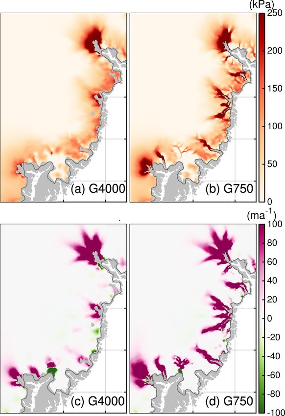
3310                                         M. Rückamp et al.: Resolution effects of AWI ISMIP6 Greenland projections

    While the relative importance of outlet glacier discharge
for total GrIS mass loss has decreased since 2001 (Enderlin
et al., 2014; Mouginot et al., 2019) and is expected to de-
crease further in the future (e.g. Aschwanden et al., 2019),
it remains an important aspect for projecting future sea-level
contributions from the ice sheet on the centennial timescale
(Goelzer et al., 2013; Fürst et al., 2015). A (non-linear) dy-
namic response of the ice sheet is caused by changes in the at-
mospheric and oceanic forcing that may trigger glacier accel-
eration and thinning of outlet glaciers. Moreover, processes
such as SMB and ice discharge are mutually competitive in
removing mass from the ice sheet (Goelzer et al., 2013; Fürst
et al., 2015). Beside this interplay, a simple extrapolation of   Figure 1. Results from the initMIP-Greenland exercise (Goelzer
observed GrIS mass loss trends over the next century is not       et al., 2018). Sea-level contribution vs. (minimum) horizontal grid
justified, as high temporal variations in SMB and glacier ac-     resolution of each participating ISM. Equal model versions but dif-
celeration are apparent (e.g. Moon et al., 2012). Therefore,      ferent grid resolutions are connected with a coloured line. ISSM
reliable ice sheet models (ISMs) forced with future-climate       model versions are connected with a coloured dashed line. Note the
data must be driven for policy-relevant sea-level projections     logarithmic scale of the x axis. For unstructured meshes the finest
on century timescales.                                            resolution is displayed.
    The Ice Sheet Model Intercomparison Project (ISMIP6;
Nowicki et al., 2016, 2020a) is an international commu-
nity effort striving to improve sea-level projections from the       Interestingly, the estimated sea-level contributions show a
Greenland and Antarctic ice sheets. Based on previous ef-         dependence on grid resolution (Fig. 1). ISM versions with
forts like SeaRISE (Bindschadler et al., 2013; Nowicki et al.,    multiple grid resolutions demonstrate that coarser grid reso-
2013) and ice2sea (e.g. Gillet-Chaulet et al., 2012), ISMIP6      lutions tend to produce a slightly larger mass loss. This ef-
continues to fully explore the sea-level rise contribution and    fect is partly due to the methodological approach by con-
associated uncertainties. The effort is aligned with the Cou-     sidering an SMB anomaly that is based on the present-day
pled Model Intercomparison Project Phase 6 (CMIP6; Eyring         observed SMB. That means ISMs with initial areas larger
et al., 2016) to provide input for the upcoming assessment        than those observed are subject to more and stronger melting
report of the Intergovernmental Panel on Climate Change           and sharper transitions in SMB. Therefore, coarse-resolution
(IPCC AR6). The general strategy is to use outputs from           models not rendering the present-day ice margin perfectly
CMIP5 and CMIP6 climate models to derive atmosphere and           will likely overestimate ablation.
ocean fields for forcing ISMs. Goelzer et al. (2020a) and            However, increasing the spatial resolution comes with the
Nowicki et al. (2020b) analyse the future sea-level contri-       ability to resolve the geometry and to track outlet glacier
bution from multi-model ensembles for ISMIP6-Projections-         behaviour (Greve and Herzfeld, 2013; Aschwanden et al.,
Greenland. The major aim of Goelzer et al. (2020a) is to pro-     2016). Some previous works have focused on the dependence
vide future sea-level change projections and related uncer-       of future mass loss of the GrIS on grid resolution (Greve and
tainty in a consistent framework.                                 Herzfeld, 2013; Aschwanden et al., 2019). In these studies
    Despite substantial progress in ice sheet modelling in the    no clear conclusion on how the resolution affects the mass
last few decades and years, a challenging goal remains to         loss was found. This was partly explained by the compet-
narrow uncertainties and improve the reliability of future        ing tendencies of SMB and ice discharge that are differently
sea-level projections from the two big ice sheets. To date,       resolved by the adopted resolutions. A separation of both
it is recognized that the largest uncertainty sources are re-     responses in future-projection experiments would elucidate
lated to the initialization of the ISM or stem from external      how these two main sea-level contributors from the GrIS are
forcing (Goelzer et al., 2018, 2020a). Goelzer et al. (2018)      affected by the horizontal resolution. Most likely coarse grids
compared the initialization techniques used by different ice-     underestimate ice discharge as ice flow patterns and cross
sheet-modelling groups. The schematic forward experiment          sections of outlet glacier geometries are not well captured
was not designed to estimate realistic sea-level contribution,    (Greve and Herzfeld, 2013; Aschwanden et al., 2016). High-
but it provides valuable insights into how the initial state of   resolution models, in turn, require a larger amount of com-
an ISM affects the ice sheet response. Under a predefined         putational resource. Unfortunately, when increasing the res-
SMB anomaly, mass losses reveal a large spread. Although          olution, simple approximations to the momentum balance do
the spread is attributed to the broad diversity in model ap-      not provide an accurate solution (Pattyn et al., 2008). This
proaches, initMIP-Greenland shows notable improvements            limitation takes place particularly at the ice sheet margin and
(e.g. a reduced model drift) and more consistent results com-     at outlet glaciers where all terms in the force balance become
pared to earlier large-scale intercomparison exercises.           equally important (e.g. Pattyn and Durand, 2013). Due to the

The Cryosphere, 14, 3309–3327, 2020                                                   https://doi.org/10.5194/tc-14-3309-2020
M. Rückamp et al.: Resolution effects of AWI ISMIP6 Greenland projections                                                   3311

intensive computational resources needed to solve the full-      use variable ice flow approximations ranging from shallow-
Stokes equation, higher-order (HO) approximations provide        ice approximation to full Stokes and also has the capability to
a good compromise to balance model accuracy and compu-           perform inverse modelling to constrain unknown parameters.
tational costs on centennial timescales.                            Here, we make use of the Blatter–Pattyn approximation
   Determining whether increased model resolution is worth       (Blatter, 1995; Pattyn, 2003) to obtain the most accurate so-
the extra computation time would be valuable to make             lution even though computational time is increased compared
progress in narrowing uncertainties in ice sheet projections,    to simpler models (e.g. Aschwanden et al., 2019). The system
even if only by a few per cent. The ISMIP6-Projections-          of equations is solved numerically with the finite-element
Greenland shows that models with low and high resolution         method, and state variables are computed on each vertex
are found at the upper and lower bound of sea-level contri-      of the mesh using piecewise linear finite elements. The ice
bution, though no specific analysis of the grid resolution has   rheology is treated with a regularized Glen flow law (Glen,
been performed.                                                  1955), a temperature-dependent rate factor for cold ice and
   The main intention of this paper is to complement the         a water-content-dependent rate factor for temperate ice (Lli-
study by Goelzer et al. (2020a) by evaluating the sensitivity    boutry and Duval, 1985).
of the simulated GrIS response to global warming due to dif-        At the ice base, sliding is allowed everywhere and the
ferent horizontal grid resolutions by one single ISM. Besides    basal drag τb follows a linear viscous law (Weertman, 1957;
running the full scenarios (i.e. both oceanic and atmospheric    Budd et al., 1984):
forcing considered), we aim to explore the grid-resolution
                                                                 τb,i = −k 2 N vb,i ,                                         (1)
dependence on atmospheric and ocean forcing separately.
Therefore, the full scenarios are complemented with exper-       where vb,i is the basal velocity vector in the horizontal plane
iments where either a changing SMB or the interaction of         and i = x, y. Although this type of friction law is often used
the glacier with the ocean is omitted. The simulations of the    in ice sheet modelling (Morlighem et al., 2010; Price et al.,
GrIS are performed with the Ice-sheet and Sea-level System       2011; Gillet-Chaulet et al., 2012; Seroussi et al., 2013), it im-
Model (ISSM; Larour et al., 2012) and adopted spatial reso-      plies that the basal drag can increase without a bound. It was
lutions ranging from medium to high (4 and 0.75 km at fast-      shown that inducing an upper ratio of τb /N (Iken’s bound) is
flowing outlet glaciers, respectively). The future scenarios     more justified (Iken, 1981; Schoof, 2005; Gagliardini et al.,
build on climate-forcing data from the CMIP5 global circula-     2007; Leguy et al., 2014; Joughin et al., 2019). However, we
tion model (GCM) MIROC5 under the Representative Con-            choose this type of friction law as it is commonly used in
centration Pathway (RCP) 8.5 (Moss et al., 2010) following       ISMs making use of inverse methods to constrain the basal
the ISMIP6 protocol (Nowicki et al., 2020a).                     friction (Morlighem et al., 2010; Larour et al., 2012; Seroussi
                                                                 et al., 2013; Perego et al., 2014; Gladstone et al., 2014).
                                                                    The friction coefficient k 2 is assumed to cover bed prop-
2     Methods and experiments                                    erties such as bed roughness. The effective pressure is de-
                                                                 fined as N = %i g h+min(0, %w g zb ), where h is the ice thick-
Before presenting the concept of this study, we aim to ad-       ness; zb is the glacier base; and %i = 910 kg m−3 and %w =
dress the terminology used for clarity. Following the glos-      1028 kg m−3 are the densities for ice and seawater, respec-
sary in Cogley et al. (2011), ice discharge is computed as the   tively. The parameterization accounts for full water-pressure
product of ice thickness h and the depth-averaged velocity v̄.   support from the ocean wherever the ice sheet base is be-
In the following, the lower-case q (Gt a−1 m2 ) refers to the    low sea level, even far into its interior where such a drainage
local ice discharge at a point and the upper-case Q (Gt a−1 )    system may not exist. At marine-terminating glaciers, water
refers to the glacier-wide quantity (analogous to other quan-    pressure is applied, and zero pressure is applied along land-
tities such as glacier-wide calving D and local calving d).      terminating ice cliffs. A traction-free boundary condition is
Quantities at the margin are reckoned to be in the normal di-    imposed at the ice–air interface.
rection.                                                            The ISSM model domain for the Greenland ice sheet
                                                                 covers the present-day main ice sheet extent and includes
2.1    Ice flow model ISSM                                       the current floating ice tongues (e.g. Petermann, Ryder and
                                                                 79◦ N glaciers). The geometric input is BedMachine v3
The model applied here is the Ice-sheet and Sea-level Sys-       (Morlighem et al., 2017). The thickness, bedrock and ice
tem Model (ISSM; Larour et al., 2012). It has been applied       sheet mask is clipped to exclude glaciers and ice caps sur-
successfully to the GrIS in the past (Seroussi et al., 2013;     rounding the main ice sheet. The initial ice sheet mask
Goelzer et al., 2018; Rückamp et al., 2018, 2019a) and is        is manually retrieved from the data coverage of the MEa-
also used for studies of individual drainage basins of Green-    SUREs velocity data set (Joughin et al., 2016, 2018) to en-
land, e.g. the Northeast Greenland Ice Stream (Choi et al.,      sure an available target for the basal-friction inversion em-
2017), Jakobshavn Isbræ (Bondzio et al., 2017) and Peter-        ployed (Sect. 2.3). A minimum ice thickness of 1 m is ap-
mann Glacier (Rückamp et al., 2019b). ISSM is designed to        plied. Grounding-line evolution is treated with a subgrid pa-

https://doi.org/10.5194/tc-14-3309-2020                                                 The Cryosphere, 14, 3309–3327, 2020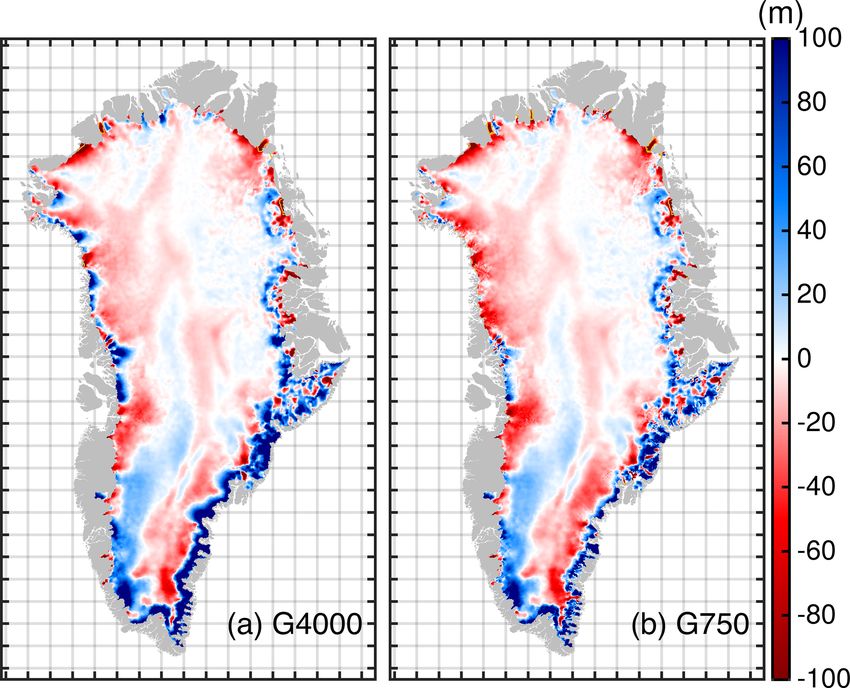
3312                                          M. Rückamp et al.: Resolution effects of AWI ISMIP6 Greenland projections

rameterization scheme, which tracks the grounding-line posi-
tion within the element (Seroussi et al., 2014). A subgrid pa-
rameterization on partially floating elements for basal melt is
applied (Seroussi and Morlighem, 2018). The basal-melt rate
below floating tongues is parameterized with a Beckmann–
Goosse relationship (Beckmann and Goosse, 2003). In this
parameterization ocean temperature and salinity are set to
−1.7 ◦ C and 35 Psu, respectively. The melt factor is roughly
adjusted such that melting rates correspond to literature val-
ues (e.g. Wilson et al., 2017; Rückamp et al., 2019b). How-
ever, at most locations the grounding line coincides with the
calving front. Except for the floating-tongue glaciers Peter-
mann, Ryder and 79◦ N, the subgrid schemes at the ground-
ing line are not applied. The treatment of the calving-front
evolution depends on the experimental setup and is explained
in Sect. 2.4 and 2.5.2.
   As we expect the grounding line not to retreat too exces-
                                                                   Figure 2. Horizontal mesh resolution (km) used for G4000 (a) and
sively in the projections, model calculations with ISSM are        G750 (b). Data are clipped at 0.5 and 10 km. The horizontal res-
performed on a horizontally unstructured grid which remains        olution of a triangle is defined by its minimum edge length. The
fixed in time. To limit the number of elements while max-          grey line delineates the initial ice domain. Grey grid lines indicate
imizing the horizontal resolution in regions where physics         100 km. The black boxes indicate the northwestern and southeast
demands higher accuracy, the horizontal mesh is generated          subsets used in following figures.
with a higher resolution of REShigh in fast-flowing regions
(observed ice velocity > 200 m a−1 ) and a coarser resolution
of RESlow in the interior. This adaptive strategy allows a vari-
able resolution in key areas of the ice sheet, e.g. marine-
terminating outlet glaciers. Experiments are carried out at
four different horizontal grid resolutions with REShigh equal
to 4, 2, 1 and 0.75 km (Table 1 and Fig. 2). The distribution
of mesh vertices at numerous outlet glaciers is depicted in
Figs. S6 to S19 in the Supplement. In Fig. 3, the interpolated
bed elevation for two selected regions and grid resolutions is
illustrated. Overall, the bedrock topography of the finer res-
olution shows deeper and fjord-like troughs, which is closer
to the BedMachine data set.
   Independent of the horizontal resolution, the vertical dis-
cretization comprises 15 terrain-following layers, refined to-
wards the base where vertical shearing becomes more im-
portant. Please note that G1000 and G750 correspond to the
ISMIP6 contributions AWI-ISSM2 and AWI-ISSM3, respec-
tively, in Goelzer et al. (2020a).

2.2    Overview of experiments

The ISMIP6 protocol requests the initialization mode prior
to or on the ISMIP6 projection start date. If the initialization
date is before the start of the projections, a short historical
run is needed to advance the ISM from the reference date to
the end of 2014. From this date, the future-climate scenarios
branch off. Unforced constant-climate control experiments          Figure 3. G4000 and G750 bedrock topography for the northwest-
are defined to capture the model drift with respect to the ISM     ern region (a, b, respectively), and for the southeast region (c, d,
reference climate and the ISMIP6 projection start date. The        respectively). Region subsets are shown in Fig. 2.
set of experiments are described in the following sections but
can be summarized as follows:

The Cryosphere, 14, 3309–3327, 2020                                                     https://doi.org/10.5194/tc-14-3309-2020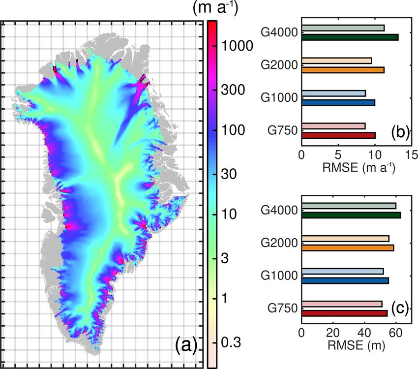
M. Rückamp et al.: Resolution effects of AWI ISMIP6 Greenland projections                                                                  3313

Table 1. Summary of models and their mesh characteristics. Computational time is based on a projection run under MIROC5 RCP 8.5 and
medium ocean forcing.

                     Model name        REShigh       RESlow        Number of        Time step       Computational        Number of
                                         (km)          (km)         elements        1t (years)         time (min)            cores
                     G4000                     4           7.5      1 169 546             0.100                  83              90a
                     G2000                     2           7.5      1 951 586             0.050                 252             162a
                     G1000                     1           7.5      4 241 020             0.025                 640             342b
                     G750                   0.75           7.5      6 220 928             0.010                1731             702b
                   a Intel Xeon Broadwell CPU E5-2697 v4, 2.3 GHz, on the AWI cluster system Cray CS400.
                   b Intel Xeon Broadwell CPU E5-2695 v4, 2.1 GHz, on the German Climate Computing Center (DKRZ) cluster system Mistral.

  – Initialization. Experiment to retrieve the initial state of                  by Seroussi et al. (2013) and Goelzer et al. (2018, see sub-
    the model is performed.                                                      missions AWI-ISSM1 and 2) that the temperature field and
                                                                                 its change have a negligible effect on century timescale pro-
  – ctrl. Experiment where the climate is held constant to                       jections of the GrIS.
    the reference climate (from January 1991 to end of De-                          The main ingredient of the initialization is the inver-
    cember 2100) is performed.                                                   sion to infer the basal-friction coefficient k 2 in Eq. (1).
                                                                                 This approach minimizes a cost function that measures the
  – ctrl_proj. Experiment where the climate is held constant                     misfit between observed and modelled horizontal velocities
    to the reference climate (from January 2015 to end of                        (Morlighem et al., 2010). The cost function is composed of
    December 2100) is performed.                                                 two terms which fit the velocities in fast- and slow-moving
  – Historical. Experiment to bring model from the initial-                      areas. A third term is a Tikhonov regularization to avoid
    ization state to the ISMIP6 projection start date (from                      oscillations. The parameters for weighting the three contri-
    January 1991 to end of December 2014) is performed.                          butions to the cost function are taken from Seroussi et al.
                                                                                 (2013). We leverage horizontal surface velocities from the
  – Projection. Future-climate scenario (from January 2015                       MEaSUREs project (Joughin et al., 2016, 2018), as the data
    to end of December 2100) is projected.                                       set with almost no gaps over the GrIS is suitable for basal-
                                                                                 friction inversion.
2.3   Initialization experiment                                                     The assigned reference year is 1990. This date is not in
                                                                                 agreement with the timestamps of the BedMachine data set
The initialization state of ISSM is based on data assimilation                   (reference time is 2007) and the MEaSUREs velocity data set
and inversion for determining the basal-friction coefficient.                    (temporal coverage from 2014 to 2018). However, we ignore
Before the inversion, a relaxation run assuming no sliding                       the contemporaneity requirement in the inversion approach
and a constant ice temperature of −10 ◦ C is performed to                        and put more weight on starting the projections at the end
avoid spurious noise that arises from errors and biases in the                   of the assumed GrIS steady-state period (e.g. Ettema et al.,
data sets. To ensure that the relaxed geometry does not de-                      2009). All transient simulations start from the initial state;
viate too much from the observed geometry, the relaxation                        that means, we do not perform a subsequent relaxation run to
is conducted over 1 year. However, while inverse modelling                       bring the model to a steady state (see Sect. 2.6).
is well established for estimating basal properties, the tem-
perature field is difficult to constrain without performing an                   2.4    Historical and control experiments
interglacial thermal spin-up. Therefore, we rely on a tem-
perature field that was obtained by a hybrid approach be-                        In both control experiments (ctrl and ctrl_proj), the SMB and
tween palaeoclimatic thermal spin-up and basal-friction in-                      ice sheet mask remain unchanged from the reference year ac-
version. This method was developed for the AWI contribu-                         cording to the ISMIP6 protocol. To advance the model from
tion in initMIP-Greenland (Goelzer et al., 2018) and further                     the reference time to the projection start date, the histori-
improved in Rückamp et al. (2018) by using the geothermal                        cal scenario is needed. During the historical period, yearly
flux pattern from Greve (2005, scenario hf pmod2). Here,                         cumulative SMB is taken from the RACMO2.3p2 product
we initialize the ice rheology on the four employed G4000–                       (Noël et al., 2018) for the years from 1990 to 2015. For sim-
G750 grids by interpolating the 3-D temperature and water                        plicity, the ice sheet extent remains unchanged from the ref-
content fields from the hybrid spin-up in Rückamp et al.                         erence year. This is a crude approach, but representing the
(2018). The basal-melting rates of grounded ice are equiv-                       historical mass loss accurately was not a strong priority for
alently interpolated. During all transient runs, we neglect an                   our experimental setup. As the ice front is not moving in
evolution of the thermal field. This is justified as it was shown                these three scenarios, ice discharge Q equals calving D.

https://doi.org/10.5194/tc-14-3309-2020                                                                     The Cryosphere, 14, 3309–3327, 2020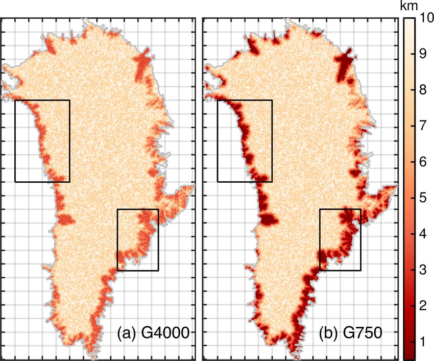
3314                                         M. Rückamp et al.: Resolution effects of AWI ISMIP6 Greenland projections

2.5     Future forcing experiments

It is beyond the scope of this paper to present the details of
the ISMIP6 protocol and experimental design. Therefore, we
aim to briefly outline the external-forcing approach. Further
details are given in Goelzer et al. (2020a), Nowicki et al.
(2020a), Fettweis et al. (2020) and Slater et al. (2019, 2020).
   As we aim to study the effect of grid resolution on ice
mass changes, we run the future scenarios based on climate
data from one single GCM. The GCM MIROC5 was se-
lected as it performs well in the historical period and rep-
resents a plausible climate near Greenland (Barthel et al.,
2020). The GCM output is used to separately derive ISM
forcing for the interaction with the atmosphere and the ocean.
We set up experiments where both external forcings are con-
                                                                  Figure 4. Atmospheric and oceanic forcing. (a) Spatial pattern
sidered; these scenarios are termed “full” in the following
                                                                  of the cumulative (2015–2100) SMB anomaly based on MIROC5
(RCP8.5-Rlow, RCP8.5-Rmed, RCP8.5-Rhigh). In addition,            RCP 8.5 and downscaled with MAR (Fettweis et al., 2020). (b) Re-
we perform simulations where either the atmospheric forc-         treat of marine-terminating outlet glaciers in the northwestern re-
ing (RCP8.5-Rnone) or the marine-terminating outlet glacier       gion under RCP8.5-Rhigh scenario. Purple areas indicate retreated
retreat (OO-Rmed, OO-Rhigh) is at play. The conducted pro-        areas in 2100. Region subsets are shown in Fig. 2.
jection experiments and the corresponding experiment labels
used in this study are summarized in Table 2 and are ex-
plained in the following sections.                                The SMB height–elevation feedback is considered with a dy-
                                                                  namic correction SMBdyn to the SMBclim following Franco
2.5.1    Atmospheric forcing                                      et al. (2012):

ISMIP6 provides surface-forcing data sets for the GrIS based      SMBdyn (x, y, t) = dSMBdz(x, y, t) × (zs (x, y, t)
on CMIP GCM simulations. The GCM output is dynamically                              − zref (x, y)).                               (4)
downscaled through the higher-resolution regional climate
model (RCM) MAR v3.9 (Fettweis et al., 2017). The latter          The surface elevation changes are taken from the ISM ele-
allows for the capturing of narrow regions at the periphery of    vation zs (x, y, t) while running the simulation and the cor-
the Greenland ice sheet with large SMB gradients, which are       responding ISM reference elevation zref (x, y) from the ini-
likely not captured by the GCMs. The climatic SMB that is         tialization state. The yearly patterns of 1SMB(x, y, t) and
used as future-climate forcing reads                              dSMBdz(x, y, t) are provided by ISMIP6. A cumulative
                                                                  SMB anomaly over the projection period is shown in Fig. 4a.
SMBclim (x, y, t) = SMBref (x, y) + 1SMB(x, y, t)
                                                                  2.5.2   Oceanic forcing
                  + SMBdyn (x, y, t),                      (2)
                                                                  For the oceanic forcing we rely on the empirically derived
with the anomaly defined as                                       outlet glacier parameterization retreat by Slater et al. (2019,
                                                                  2020). This method circumvents the problem of employing a
1SMB(x, y, t) = SMB(x, y, t)GCM–MAR                               physically based calving law and frontal-melting rates based
                − SMB(x, y)1960−1989
                           GCM–MAR ,                       (3)    on GCM output. When employing this parameterization to
                                                                  the calving front, retreat and advance of marine-terminating
where SMB(x, y, t)GCM–MAR is the direct output of MAR us-         outlet glaciers is directly prescribed as a yearly series of ice
ing the GCM climate data and SMB(x, y)1960−1989
                                            GCM–MAR the cor-      front positions. (i.e. it is not a result of the ice velocity at the
responding mean value over the reference period (from Jan-        calving front, calving rate and frontal melt that are used to
uary 1960 to December 1989). As the reference SMB field           simulate the calving-front position). Here, the binary retreat
SMBref (x, y), we choose the downscaled RACMO2.3p2                masks (i.e. ice-covered and non-ice-covered cells) are inter-
product (Noël et al., 2018) whereby a model output was            polated to the native grid by nearest-neighbour interpolation.
averaged for the period 1960–1990. This period is chosen          Retreat occurs once a cell is fully emptied.
as the ice sheet is assumed to be close to a steady state in         Though this parameterization is a strong simplification, it
this period. (e.g. Ettema et al., 2009). The SMB deduced by       builds on projected sub-marine melting taking into account
MAR is processed on a fixed topography (off-line); conse-         changes in ocean temperature and surface meltwater runoff
quently local climate feedback processes due to the evolv-        from a GCM. The parameterization is not applied to the in-
ing surface in the projection experiments are not captured.       dividual glaciers but over a predefined geographical region.

The Cryosphere, 14, 3309–3327, 2020                                                    https://doi.org/10.5194/tc-14-3309-2020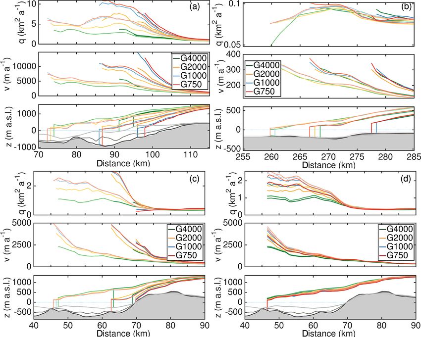
M. Rückamp et al.: Resolution effects of AWI ISMIP6 Greenland projections                                                        3315

Table 2. Summary of projection experiments based on MIROC5 RCP 8.5 climate data.

                            Experiment label    Atmospheric forcing    Oceanic forcing    Combination
                            RCP8.5-Rlow         SMB anomaly            low                full
                            RCP8.5-Rmed         SMB anomaly            med                full
                            RCP8.5-Rhigh        SMB anomaly            high               full
                            RCP8.5-Rnone        SMB anomaly            –                  atmospheric only
                            OO-Rmed             –                      med                ocean only
                            OO-Rhigh            –                      high               ocean only

Based on the numerous retreat trajectories, a medium retreat          3     Results
scenario as the trajectory with the median retreat in 2100
is defined. To cover uncertainty by this approach, low- and           3.1     Historical scenario
high-retreat scenarios are defined as the trajectories with the
25th and 75th percentile retreats in 2100. In the following,          To evaluate the modelling decisions pertaining to the initial-
these retreat scenarios are termed Rlow, Rmed and Rhigh               ization, the state of the ice sheet at the end of the historical
(Table 2). The retreat mask for RCP8.5-Rhigh in 2100 is               period is compared to observations. Due to the sparseness
exemplarily shown in Fig. 4b. Please note that the future-            and limited temporal and spatial coverage of available obser-
projection experiment RCP8.5-Rnone experiences no retreat             vations, we rely on the BedMachine v3 (150 m grid spacing)
of marine-terminating outlet glaciers.                                and MEaSUREs (250 m grid spacing) data sets for ice thick-
                                                                      ness and surface velocity, respectively. As these data are used
2.6   Comparability of experiments                                    in the data assimilation and inversion, velocity and thickness
                                                                      are not independent quantities. However, during the histori-
Central questions about resolution dependence are always as           cal period the ice sheet state is altered by the boundary con-
follows: how comparable are the results, and what is con-             ditions and external forcing. Therefore, the following evalu-
trolling the results? The presented initialization procedure          ation attempts to quantify differences from the model config-
and involved parameters are achieved for the high-resolution          urations on the ISMIP6 projection start date.
simulations (G750). The simulations with a coarser resolu-               Since the results are qualitatively similar for each grid sim-
tion would probably require other parameters, e.g. to obtain a        ulation (Figs. S1, S2 and S3 in the Supplement), the surface
better result for observational targets or to achieve a reduced       velocity field of the G750 simulation is exemplarily shown
model drift. However, we decided here to keep model param-            in Fig. 5a. A consequence of the employed basal-friction
eters (e.g. inversion parameters) and parameterizations (e.g.         inversion is the high fidelity in simulating the observed-
subgrid scheme at grounding line) unchanged for all simula-           velocity field indicated by a low root mean square error
tions. Similarly to the retreat masks, we rely on binary retreat      (RMSE; Fig. 5b). Notable is the decreasing RMSE with in-
masks for all adopted resolutions although the ISMIP6 proto-          creasing spatial resolution. At the end of the historical exper-
col requests a subgrid scheme for coarse-resolution models.           iment the RMSE is increased compared to the initialization
On the one hand this strategy simply assumes that the results         due to geometric and velocity adjustments over the course
are comparable as they build on the same basis. On the other          of the experiment. However, the ice-sheet-wide RMSE of
hand it avoids exploring parameter spaces which are out of            each model version is very similar, but in the areas of fast-
the scope of this study.                                              flowing outlet glaciers (observed velocity > 200 m a−1 ) dif-
   For the geometric input we are following the same strat-           ferences are more evident: the G4000 and G750 simula-
egy. It is always a compromise between matching the ob-               tions yield RMSE = 150 m a−1 and RMSE = 80 m a−1 , re-
served geometry or being closer to a steady state. Here, we           spectively. Note that these values are not identical to those
put more weight on having the initial geometry closer to the          given in Goelzer et al. (2020a), as the evaluation here is based
observed geometry. Therefore, we directly started the histor-         on a different subsampling method. A mean signed differ-
ical run after the inversion, and no further relaxation run is        ence (MSD) reflects a stronger underestimation of the simu-
performed to bring the model to a steady state. As the model          lated velocities with coarser resolution. The underestimation
is likely not in a steady state at the initial state, we expect a     of prominent outlet glaciers for the G4000 setup is demon-
model drift in the transient runs which would not be the case         strated in the spatial pattern of velocity differences (Fig. S4
for models that perform a relaxation towards a steady state           in the Supplement). With increasing resolution, the differ-
after the inversion.                                                  ence pattern becomes more heterogeneous. Although barely
                                                                      visible, the G750 setup provides an interesting signature at
                                                                      narrowly confined outlet glaciers: generally, the velocities in
                                                                      the main trunk are underestimated, while beneath the shear

https://doi.org/10.5194/tc-14-3309-2020                                                     The Cryosphere, 14, 3309–3327, 2020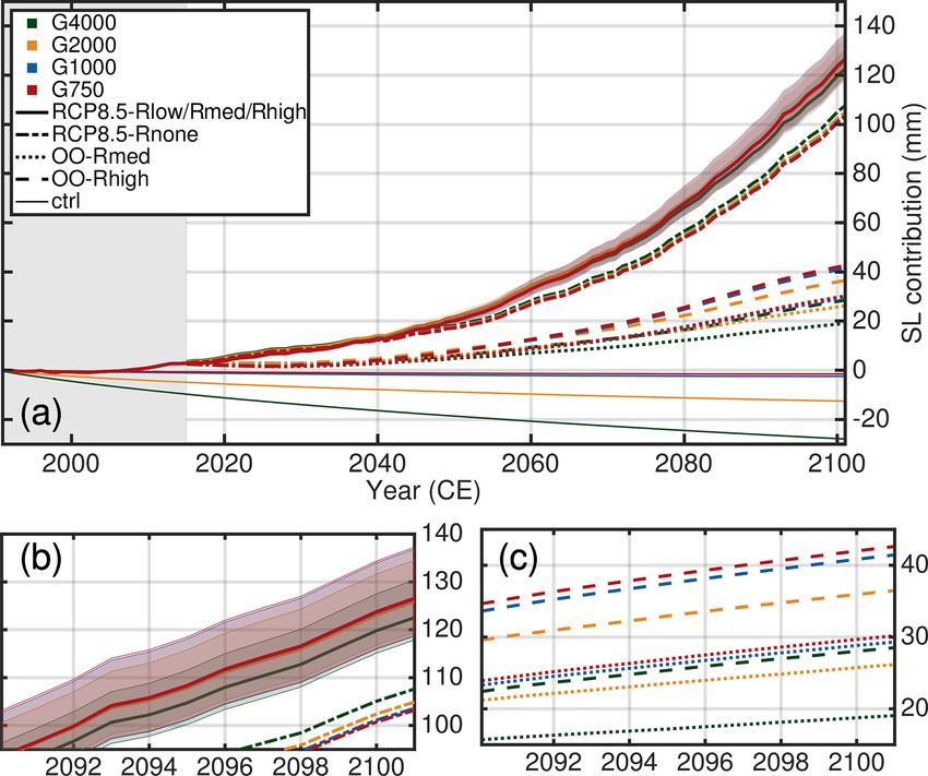
3316                                              M. Rückamp et al.: Resolution effects of AWI ISMIP6 Greenland projections

Figure 5. Simulation results and error estimate of model output at
the end of the historical run compared to observations. (a) Simu-
lated surface velocity of the GrIS (m a−1 ) from the G750 simula-
                                                                        Figure 6. Projected sea-level contribution of the Greenland ice
tion. The grey silhouette shows the Greenland land mask from Bed-
                                                                        sheet based on MIROC5 RCP 8.5 climate data (a). Coloured lines
Machine v3. Thin black lines show the grounding line. (b) Root
                                                                        indicate the different grid resolutions employed, while the individ-
mean square error (RMSE) of the horizontal velocity magnitude
                                                                        ual scenarios are indicated with different line styles. The mass loss
compared to MEaSUREs. (c) RMSE of ice thickness (not corrected
                                                                        trends are corrected with the ctrl run relative to the reference time.
with ctrl) compared to BedMachine v3. In panels (b) and (c), light
                                                                        The grey-shaded box shows the historical period. (b) Enlargement
and dark colours represent diagnostics at the initialization and end
                                                                        of the RCP8.5-Rlow, RCP8.5-Rmed, RCP8.5-Rhigh and RCP8.5-
of the historical experiment, respectively. The diagnostics have been
                                                                        Rnone scenarios. (c) Enlargement of the OO-Rmed and OO-Rhigh
calculated on the regular MEaSUREs and BedMachine grids, re-
                                                                        scenarios.
spectively.

                                                                        3.2   Sea-level contribution
margin velocities are overestimated. This might be due to the
fact, that the employed resolution is not able to resolve the
                                                                        In the following the transient effect of spatial resolution
sharp velocity jump across the shear margin.
                                                                        on ice volume evolution for the future-climate experiments
   A similar evaluation for the thickness is performed. The
                                                                        is studied. The change in ice mass loss is expressed as
ice-sheet-wide RMSE of ice thickness depicts the qualita-
                                                                        sea-level contributions. Therefore, the simulated volume
tively similar grid-dependent behaviour as the velocity eval-
                                                                        above flotation is converted into the total amount of global
uation (Fig. 5c). Similarly, the RMSE shows larger differ-
                                                                        sea-level equivalent by assuming a constant ocean area of
ences in the fast-flow regions: the G4000 and G750 simula-
                                                                        3.618 × 10⁸ km2 . In the following, the mass losses in the
tions yield RMSE = 126 m and RMSE = 45 m, respectively.
                                                                        projection experiments are corrected with the ctrl run with
In this region, the MSD indicates underestimation of ice
                                                                        respect to the reference time. For all conducted projection
thicknesses with coarser resolution. Spatial patterns of the
                                                                        experiments, the determined GrIS mass losses as a function
thickness differences over the course of the historical exper-
                                                                        of time are shown in Fig. 6 and listed in Table 3.
iment are shown in Fig. S5 in the Supplement.
                                                                           As we have not initialized our model to be at a steady state,
   The stored volumes, ice extent and spatially inte-
                                                                        the transient response in the ctrl experiment (thin coloured
grated SMB are among all grid simulations rather simi-
                                                                        lines in Fig. 6) should not be interpreted as a prediction of
lar (V = 7.28 m SLE ± 0.2 %, A = 1.787 × 10⁶ km2 ± 0.7 %,
                                                                        actual future behaviour; the ctrl run rather confirms that each
SMB = 375 Gt a−1 ± 0.2 %). However, the underestimation
                                                                        model has achieved a high degree of equilibration, which is
of velocities and ice thicknesses in the coarser-resolution
                                                                        reflected by a low rate of volume change. As the initialization
models is confirmed by the temporal mean of the ice dis-
                                                                        states are presumably different across the employed grids,
charge in the historical period. The intrinsically simulated
                                                                        we expect a different response of the ice sheet as it is likely
ice discharge Q yields 207 to 341 Gt a−1 for the G4000 and
                                                                        not in equilibrium with the applied SMB and ice flux diver-
G750 simulations, respectively.
                                                                        gence. The simulated ice mass evolution shows for all mod-
                                                                        els a mass gain for the 111-year ctrl experiment ranging be-
                                                                        tween −28 and −2 mm. With increasing resolution, the drift
                                                                        gets smaller and is minimal for the G1000 and G750 simu-
                                                                        lations. Although projections are corrected with the ctrl run,

The Cryosphere, 14, 3309–3327, 2020                                                          https://doi.org/10.5194/tc-14-3309-2020
M. Rückamp et al.: Resolution effects of AWI ISMIP6 Greenland projections                                                                            3317

Table 3. Modelled mass change (mm SLE) in future experiments
for all experiments.

  Experiment label                     G4000         G2000        G1000        G750
  Corrected with ctrl∗
  RCP8.5-Rlow                            118.3        119.7        118.6       118.7
  RCP8.5-Rmed                            122.5        125.8        126.4       126.5
  RCP8.5-Rhigh                           130.8        134.7        136.8       137.2
  RCP8.5-Rnone                           108.0        105.1        103.6       103.1
  OO-Rmed                                 19.5         26.4         29.3        30.1
  OO-Rhigh                                28.9         36.7         41.4        42.6
  Corrected with ctrl_proj∗
  RCP8.5-Rlow                            115.8        117.6        117.1       117.2
  RCP8.5-Rmed                            120.0        123.7        124.8       125.1
  RCP8.5-Rhigh                           128.3        132.6        135.3       135.8   Figure 7. Difference in ice thickness between 2100 and 2015 for the
  RCP8.5-Rnone                           105.5        103.0        101.8       101.4   ctrl run. (a) G4000 simulation and (b) G750 simulation. The grey
  OO-Rmed                                 17.0         24.3         27.7        28.7   silhouette shows the Greenland land mask from BedMachine v3.
  OO-Rhigh                                26.5         34.6         39.9        41.1   Positive values represent thickening, and negative values show thin-
                                                                                       ning. Thin yellow line shows the grounding line in the year 2100.
  ctrl                                  −28.0        −12.6          −2.5        −1.5
  ctrl_proj                             −19.1         −8.7          −2.4        −1.9
∗ Numbers for G1000 and G750 are different compared to Goelzer et al. (2020a) as       high-emission scenario. For RCP8.5-Rmed the mass loss
they are differently calculated (e.g. considered ocean area, native vs. interpolated   reaches about 125.3 mm in 2100 (mean over G4000, G2000,
grid resolution).
                                                                                       G1000 and G750 results). The uncertainty quantification in
                                                                                       the oceanic forcing results in a mean sea-level contribution
                                                                                       that is 7.1 % less and 5.4 % greater for the RCP8.5-Rlow
the higher drift needs caution when interpreting the results                           and RCP8.5-Rhigh scenarios, respectively. When no calving-
as it has, e.g. a consequence on the SMB height–elevation                              front retreat is at play, i.e. the RCP8.5-Rnone scenario, the
feedback. The higher mass gain rates of the coarser resolu-                            projected mean mass loss is approx. 105.0 mm, i.e ∼ 20 mm
tions in the ctrl simulation are due to the lower ice discharge                        less compared to RCP8.5-Rmed. In contrast, the mean mass
rates (Sect. 3.1). Although the integrated signal in ice mass                          loss is considerably reduced to 26 and 37 mm in the OO-
change is generally small, the spatial patterns reveal an ice                          Rmed and OO-Rhigh experiment, respectively. Interestingly,
thickness imbalance of up to hundreds of metres over the                               a linear superposition of RCP8.5-Rnone and OO-Rmed leads
ctrl period (Fig. 7). Imposing an SMB correction to suppress                           to an overestimated mass loss of about 4.1 % for G4000 and
the thickness imbalance would be feasible for maintaining a                            5.3 % for G750 compared to RCP8.5-Rmed where both ex-
small drift. However, this is avoided here to enable a clean                           ternal forcings are simultaneously at play; a linear super-
comparison between the four model versions and to leave                                position of RCP8.5-Rnone and OO-Rhigh leads to 4.5 %
the ice dynamics some degree of freedom. Moreover, the                                 and 5.8 % overestimation. This is in line with earlier studies
mass trends represent an important diagnostic. Comparing                               where this effect was already reported (Goelzer et al., 2013;
the ice thickness changes reveal distinct differences between                          Fürst et al., 2015)
the grid-resolution simulations (Fig. 7). For example, at the                             Among all future projections a resolution-dependent im-
end of the ctrl run at some western and northwestern loca-                             pact on sea-level contribution is generally small compared to
tions at the margin, the G4000 simulation exhibits thickening                          the total signal for our grids. In 2100, the spread in sea-level
while the G750 reveals thinning. Another example is simu-                              contribution is 6.4 mm in RCP8.5-Rhigh, 4.1 mm in RCP8.5-
lated at the southwestern margin, where extensive thickening                           Rmed, 1.5 mm in RCP8.5-Rlow and 5 mm in RCP8.5-Rnone.
prevails in all simulations but reaches farther inland in the                          Merely the OO-Rlow and OO-Rmed scenarios exhibit a
coarser resolutions. However, from these figures, it becomes                           spread of 10.7 mm and 13.6 mm, respectively, which is on
clear that positive and negative thickness changes partially                           the order of the absolute magnitude. A notable feature for
compensate for each other, resulting in a low model drift.                             all conducted simulations is that the sea-level contribution in
   Depending on the projection scenario, the GrIS will lose                            each individual experiment converges with increasing reso-
ice corresponding to an SLE of between 19 mm (or 108 mm                                lution.
excluding OO-Rmed and OO-Rhigh) and 137 mm. For the                                       Figure 8 summarizes the qualitative behaviour of each
future-climate scenarios including atmospheric forcing a                               experiment as a function of grid resolution. Note that the
gradual increase in mass loss until the end of this cen-                               sea-level contribution in each experiment is normalized
tury is simulated, indicating accelerating mass loss for a                             by its maximum. The finer resolutions tend to produce

https://doi.org/10.5194/tc-14-3309-2020                                                                       The Cryosphere, 14, 3309–3327, 2020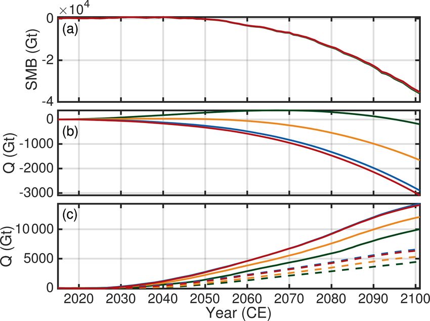
3318                                             M. Rückamp et al.: Resolution effects of AWI ISMIP6 Greenland projections

                                                                       Figure 9. Mass loss partitioning for the conducted experiments. The
                                                                       bars indicate the relative dynamic contribution to sea level, calcu-
Figure 8. Projected sea-level contribution in 2100 of the Greenland    lated as the residual of the total of the mass change and the inte-
ice sheet as a function of the horizontal grid size. Values are nor-   grated SMB anomaly. The residual is a composition of front retreat
malized to the maximum of each experiment (coloured lines). Note       and ice discharge.
the logarithmic scale of the x axis.

more mass loss in 2100 for the RCP8.5-Rmed, RCP8.5-                    ever, the importance of the dynamic contribution increases
Rhigh, OO-Rmed and OO-Rhigh experiments. An inverse                    with larger prescribed retreat rates of outlet glaciers; i.e.
behaviour is determined for the RCP8.5-Rnone experiment.               G750 with RCP8.5-Rhigh on the upper end shows the highest
The trend in the RCP8.5-Rlow experiment is not clear. The              importance of dynamic contribution with up to ∼ 28.4 %. On
RCP8.5-Rnone, OO-Rmed and OO-Rhigh experiments un-                     the lower end, the RCP8.5-Rnone shows diminished impor-
veil a linear behaviour as a function of grid size with regres-        tance of dynamic contribution (< 5 %). In the OO-Rmed and
sion slopes of m = 1.50 mm km−1 , m = −3.27 mm km−1                    OO-Rhigh scenarios, the mass loss is dominated by dynamic
and m = −4.18 mm km−1 , respectively. The trend in the full            contribution. Concerning the grid resolution, the importance
RCP8.5-Rlow, RCP8.5-Rmed and RCP8.5-Rhigh scenarios                    is on an equal level and exceeds 100 %. The negative impor-
is not consistent: RCP8.5-Rmed and RCP8.5-Rhigh show a                 tance of SMB stems from the fact that the glacier retreat is
peak in mass loss at the finest resolution, whereas a peak in          cutting off regions at the ice sheet margin where the static
mass loss is attained in the G2000 simulation for RCP8.5-              SMB is low.
Rlow. For the latter, it is worth mentioning that the varia-              In the full experiments RCP8.5-Rlow, RCP8.5-Rmed and
tions across the different grid simulations are less than 1.2 %.       RCP8.5-Rhigh, an increase in resolution enhances the im-
However, an intriguing effect of the conducted simulations             portance of the dynamic contribution. For the G750 sim-
remains the opposite behaviour of the RCP8.5-Rnone and                 ulation it is ∼ 3 %, 5 % and 6 % higher for RCP8.5-Rlow,
e.g. RCP8.5-Rhigh scenarios. In the following section, we              RCP8.5-Rmed and RCP8.5-Rhigh, respectively, compared to
study this effect by analysing the mass partition to obtain            G4000. Curiously, the opposite behaviour is observed for the
a more in-depth insight into the role of atmospheric and               RCP8.5-Rnone experiment, where a finer resolution damps
oceanic forcing on grid resolution. It is worth mentioning             the importance of the dynamic contribution; G4000 yields
that the qualitative behaviour of the detected grid-dependent          a 4.9 % dynamic contribution, whereas G750 yields a 2.9 %
mass loss remains similar when the projections are corrected           dynamic contribution.
with the ctrl_proj experiment (Table 3).                                  The simulated inverse grid-resolution responses raise the
                                                                       question of the driving causes. Overall the time series of the
3.3    Mass partitioning                                               SMB show a decline and only minor differences among the
                                                                       grid resolutions (Fig. 10a). At the end of the projection, the
The relative mass loss partitioning in 2100 is shown in Fig. 9         cumulative SMB is 2.1 % and 2.6 % lower in the G4000 sim-
to explore the role of the grid resolution in each experiment.         ulation for RCP8.5-Rnone and RCP8.5-Rhigh, respectively,
The bars indicate the relative importance to sea-level contri-         compared to G750. These differences could be explained by
bution of ice dynamic changes in the projections. The dy-              different evolution of ablation areas at the margin and the
namic contribution (composition of front retreat and ice dis-          SMB height–elevation feedback, in particular affected by the
charge) is calculated as the residual of the total mass change         ctrl run, among all grid-resolution setups. In contrast, the cu-
and the integrated SMB anomaly. The remainder explains the             mulative ice discharge for these settings reveals an oppos-
part of SMB. The overall picture reveals that for experiments          ing response in the RCP8.5-Rnone and RCP8.5-Rhigh sce-
that include the atmospheric forcing the SMB anomaly is the            narios and more relative differences between the grid resolu-
governing forcing regardless of the grid resolutions. How-             tions (Fig. 10b and c). At least for G2000, G1000 and G750,

The Cryosphere, 14, 3309–3327, 2020                                                         https://doi.org/10.5194/tc-14-3309-2020
M. Rückamp et al.: Resolution effects of AWI ISMIP6 Greenland projections 3319
coarser resolution is located above the bed of the finer resolu-
tion. This topographic effect is restricted to narrow confined
outlet glaciers that obey a characteristic width on the order
of a few kilometres. Outlet glaciers that have a larger char-
acteristic width, such as Humboldt Glacier, reveal in our se-
tups a comparable bedrock topography. These glaciers seem
to have a qualitatively equal behaviour for glacier speed-up
and change in ice discharge for all employed grid resolutions
(Fig. 11b). This analysis demonstrates that adjacent glaciers
that experience similar environmental conditions may behave
differently because ice discharge is strongly controlled by
glacier geometry.
Glaciers that are converted from a marine-terminating to a
land-terminating glacier by retreating out of the water form
Figure 10. Time series of cumulative SMB anomaly and cumu- their own class. These glaciers are no longer subject to the
lative ice discharge Q. Colour scheme is as in previous figures. retreat and show a collapse in ice discharge regardless of the
(a) Cumulative SMB anomaly for RCP8.5-Rnone. (b) Cumulative grid resolution as illustrated for Store Glacier in Fig. 11c.
ice discharge Q for RCP8.5-Rnone. (c) Ice discharge for RCP8.5- The qualitative behaviour of the retreat seems to be similar as
Rhigh (solid lines) and RCP8.5-Rlow (dashed lines). Cumulative reported in Aschwanden et al. (2019, Fig. 4b therein), but the
SMB anomaly for RCP8.5-Rhigh and RCP8.5-Rlow is qualitatively timing of the retreat is different. In our study, Store Glacier
similar to RCP8.5-Rnone. Ice discharge is not corrected with the is unstable and retreats within this century out of the water,
ctrl run. while in Aschwanden et al. (2019) Store Glacier is in a very
stable position; the quick retreat sets in far beyond 2100 once
the ice discharge in the RCP8.5-Rnone experiment decreases the glacier loses contact with the bedrock high. This different
over the century; the decrease in G4000 is offset by a few response is related to the retreat parameterization employed
decades and exhibits an increase early in the century. These that lacks information on the bedrock topography, such as
reductions explain the grid dependence of the dynamic con- topographic highs and lows.
tribution as listed in the previous paragraph (RCP8.5-Rnone RCP8.5-Rnone shows a distinct slowdown in ice veloc-
in Fig. 9). For RCP8.5-Rhigh, the ice discharge shows an in- ities as illustrated in Fig. 11d for Store Glacier. Visible is
crease consistently but is more enhanced in the finer resolu- a larger slowdown of the higher resolutions; the same be-
tions. This finding corroborates the grid-dependent increase haviour holds for the ice discharge q. This is in line with the
in the relative ice discharge importance (RCP8.5-Rhigh in finding above, i.e. that the scenario RCP8.5-Rnone reveals
Fig. 9). As the opposing differences in RCP8.5-Rnone and reduced ice discharge (Fig. 10b).
RCP8.5-Rhigh are prevailing in ice discharge, it can be con-
cluded that resolving ice discharge on the different grids is
a decisive factor here. The involved feedback are further ex- 4 Discussion
plored by focusing on particular outlet glaciers in the next
section. The simulations presented here show that the projected
sea-level contribution is sensitive to the spatial resolution.
3.4 Outlet glacier response The sensitivity effect depends on the climate forcing, with
oceanic and atmospheric forcings showing opposite and non-
The fact that the centennial mass loss for the full experiments trivial responses. The simulations have shown that the ice
increases as the grid size reduces raises the question whether discharge to the ocean is a decisive factor here controlling
this is caused by ice dynamics alone, dominant feedback with the grid-dependent spread. As shown above, outlet glaciers
surface mass balance or retreat, or other non-obvious fac- respond differently to external forcing, depending on the em-
tors. We conduct an in-depth analysis of numerous promi- ployed grids and geometrical setting. In such a non-linear
nent outlet glaciers at the GrIS (Fig. S6 and table with anal- system examining a driving mechanism remains challeng-
ysis provided as separate SI). The responses of most of the ing. However, despite the somewhat heterogeneous response
outlet glaciers reveal the deduced grid-dependent behaviour of outlet glaciers, the different scenarios tend to produce an
where higher resolutions cause an enhanced discharge. This overall trend in characteristic fields that explains the different
is exemplarily illustrated in Fig. 11a for Helheim Glacier. responses.
However, this behaviour is not visible at all selected out- The different responses in the full scenarios could be at-
let glaciers. The presented example demonstrates that the tributed to the ability to resolve bedrock topography and the
bedrock topography deviates significantly among the differ- interaction with basal sliding. Figure 12 illustrates spatial
ent grid resolutions. Generally, the bedrock topography of the changes in the effective pressure and basal-sliding velocity
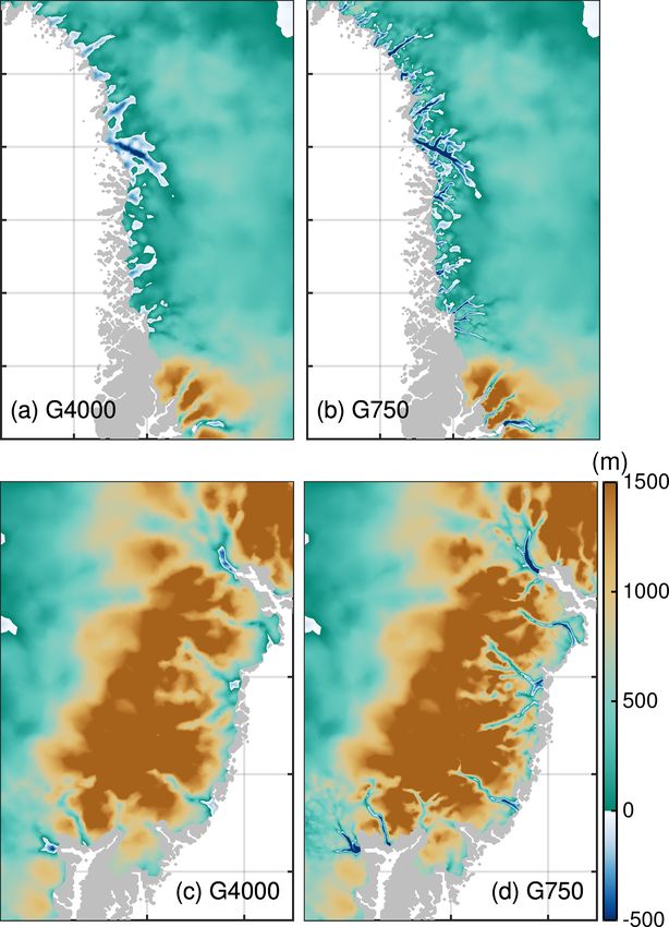
https://doi.org/10.5194/tc-14-3309-2020 The Cryosphere, 14, 3309–3327, 20203320 M. Rückamp et al.: Resolution effects of AWI ISMIP6 Greenland projections Figure 11. Response of outlet glaciers. Colour scheme is the same as in previous figures, and light to dark colours indicate the years 2015, 2070 and 2100. (a) Helheim Glacier under RCP8.5-Rhigh forcing. (b) Humboldt Glacier under RCP8.5-Rhigh forcing. (c) Store Glacier under RCP8.5-Rhigh forcing. (d) Store Glacier under RCP8.5-Rnone forcing. Upper rows show the transient behaviour of the ice discharge q, the middle rows the surface velocity v and lower rows the evolution of the ice geometry. In the lower rows, the grey-shaded area depicts the bedrock topography from the G750 simulation. The grey lines from dark to light indicate the bedrock topography from the G1000, G2000 and G4000 simulation. None of the quantities are corrected with the ctrl run. Distance is relative to an arbitrary point. for RCP8.5-Rhigh. A common characteristic for G750 is a the outlet glaciers show a speed-up, but this effect is very lo- stronger decrease in effective pressure, which is concentrated calized and does not reach far upstream. Therefore, we con- in areas where the finer grid shows a deeper bed of the marine clude, that the pronounced decrease in the effective pressure portions compared to G4000. Due to the linear dependence along with the acceleration of outlet glaciers is a dominant of τb on effective pressure (Eq. 1), basal-sliding velocities in- mechanism controlling the grid-dependent spread. crease more strongly in the finer resolution. This feedback is In order to investigate whether the response behaviour is enhanced as the SMB perturbations lead to a decrease in ice an effect of purely reducing the grid size, we repeated the thickness, hence to a decrease in the effective pressure. The OO-Rhigh and RCP8.5-Rhigh experiments with a G1000 transient evolution reveals further that thinning and acceler- simulation using regridded bedrock topography and a fric- ation propagate faster and farther upstream in the finer res- tion coefficient from the G4000 initial state (simulations are olution. The higher signal propagation rates may have addi- not shown). This setup adopts a high-resolution grid but tional consequences on longer timescales as the surface melt omits detailed information from the high-resolution input is amplified by the positive surface mass balance–elevation data. Projected mass loss by this setup is closer to the G4000 feedback exposing the ice surface to higher air temperatures. simulation. It, therefore, demonstrates that a high model res- It remains questionable if the widespread glacier acceler- olution alone is insufficient to explain the grid-dependent ation is induced by the frontal stress perturbation instead of sea-level contribution. As a consequence, a driving cause of the decrease in the effective pressure. To isolate this effect we the grid-dependent behaviour arises from additional informa- conduct a RCP8.5-Rhigh simulation (not shown) where the tion in the input data. Therefore, we conclude that the grid- effective pressure is held constant to the historical level. This dependent behaviour is highly connected to the bedrock to- setup reveals a very limited acceleration of a few glaciers pography because the different models represent the bedrock in the G4000 simulation; some show no response or even topography quite differently. a slowdown. In the corresponding G750 simulation most of The Cryosphere, 14, 3309–3327, 2020 https://doi.org/10.5194/tc-14-3309-2020
M. Rückamp et al.: Resolution effects of AWI ISMIP6 Greenland projections                                                                   3321

Figure 12. (a, b) Difference in effective pressure between 2100 and       Figure 13. (a, b) Difference in driving stress between 2100 and
2015 for the southeast region. (c, d) Difference in basal velocity be-    2015 for the northwestern region. (c, d) Difference in basal velocity
tween 2100 and 2015 for the southeast region. Region subsets are          between 2100 and 2015 for the northwestern region. Region sub-
shown in Fig. 2. Dark grey line indicates the initial ice extent. Thin    sets are shown in Fig. 2. Dark grey line indicates the initial ice ex-
black line indicating the grounding line is not visible as it falls to-   tent. Thin black line indicating the grounding line is not visible as it
gether with the calving front. The grey silhouette shows the Green-       falls together with the calving front. The grey silhouette shows the
land land mask from BedMachine v3.                                        Greenland land mask from BedMachine v3.

   Compared to the full and ocean-only scenario, the                      formed by geometric adjustments in the RCP8.5-Rnone sce-
atmospheric-only scenario unveils a stronger mass loss for                nario. This experiment intended to omit an interaction of the
the coarse resolution. To some extent, this could be explained            glacier with a changing ocean forcing, but the assumption
by a slightly lower SMB in the coarser resolution. However,               of a fixed calving front hinders outlet glaciers from adjusting
the finer resolution produces a stronger reduction in ice dis-            freely to topographic changes. They, therefore, do not experi-
charge over the course of the experiment. Although for many               ence reduced buttressing or frontal stress perturbations which
of the outlet glaciers the effective pressure decreases (not as           are necessary mechanisms to trigger widespread glacier ac-
strongly as for the scenarios with considered retreat), there is          celeration (e.g. Bondzio et al., 2017). In future studies, it
instead a slowdown of most glaciers (Fig. 13c and d). Again,              might be desirable to allow the calving front to adjust al-
these differences are concentrated in areas where the finer               though the oceanic forcing is held constant. Nevertheless,
grid shows deeper troughs. Curiously, the finer resolution                the simulations indicate that without a frontal stress perturba-
is better able to resolve these details, but the velocity evo-            tion an ensuing speed-up of the outlet glacier is not initiated.
lution causes an extra reduction in ice discharge compared                This highlights the importance of capturing calving events,
to in the coarser resolution. This non-trivial response is il-            i.e tracking the ice front position in numerical models, most
lustrated with the change in driving stress, approximated as              accurately.
τd = %i gh|gradzs | (Fig. 13a and b). Compared to 2015, the                  The inverse grid-dependent behaviour of the RCP8.5-
driving stress has locally decreased more in the finer resolu-            Rnone, OO-Rmed and OO-Rhigh scenarios has some impli-
tion in 2100 compared to the coarser resolution; away from                cations when interpreting the mass loss of the ice sheet. The
the marginal region, the driving-stress changes are on a com-             combined scenarios demonstrate that in a particular case, the
parable magnitude for all employed grids. These results in-               sea-level contribution is maximized for an intermediate reso-
dicate that the reduction in the effective pressure is outper-            lution. Depending on the horizontal grid resolution, the com-

https://doi.org/10.5194/tc-14-3309-2020                                                           The Cryosphere, 14, 3309–3327, 2020
You can also read