Semantic Labelling of Globally Distributed Urban and Non-Urban Satellite Images Using High-Resolution SAR Data

This article has been accepted for publication in a future issue of this journal, but has not been fully edited. Content may change prior to final publication. Citation information: DOI 10.1109/JSTARS.2021.3084314, IEEE Journal
 of Selected Topics in Applied Earth Observations and Remote Sensing
 JSTARS-2021-00425 1

 Semantic Labelling of Globally Distributed
 Urban and Non-Urban Satellite Images Using
 High-Resolution SAR Data
 C.O. Dumitru*, G. Schwarz, and M. Datcu

 Current approaches vary significantly from system
 Abstract—While the analysis and understanding of architectures to algorithms and data structures. The difficult
 multispectral (i.e., optical) remote sensing images has made transition to operational industrial systems is, for instance,
 considerable progress during the last decades, the automated currently taking place in Europe (e.g., Horizon 2020 [52]), at
 analysis of SAR (Synthetic Aperture Radar) satellite images still
 needs some innovative techniques to support non-expert users in
 the European Space Agency (ESA), or at national space
 the handling and interpretation of these big and complex data. In agencies (e.g., NASA, DLR, CNES, ASI).
 this paper, we present a survey of existing multispectral and SAR Existing public databases for high-resolution image sensors,
 land cover image datasets. To this end, we demonstrate how an including even commercial sensors (with the exception of
 advanced SAR image analysis system can be designed, Google [53], etc.) are very limited or even non-existing, and for
 implemented, and verified that is capable of generating the existing ones the number of discernible semantic classes is
 semantically annotated classification results (e.g., maps) as well as
 local and regional statistical analytics such as graphical charts.
 rather limited.
 The initial classification is made based on Gabor features and In this paper, we mainly concentrate on urban-oriented
 followed by class assignments (labelling). This is followed by the application cases where, at least to our knowledge, only a few
 inclusion. This can be accomplished by the inclusion of expert high-resolution and publicly available SAR (Synthetic Aperture
 knowledge via active learning with selected examples, and the Radar) reference datasets exist, while universally applicable
 extraction of additional knowledge from public databases to refine SAR reference datasets are very scarce. Therefore, a number of
 the classification results. Then, based on the generated semantics,
 we can create new topic models, find typical country-specific
 remote sensing researchers have compiled their own individual
 phenomena and distributions, visualize them interactively, and reference datasets [36].
 present significant examples including confusion matrices. This In contrast to SAR datasets, there exist several well-known
 semi-automated and flexible methodology allows several and publicly available datasets comprising a large variety of
 annotation strategies, the inclusion of dedicated analytics multispectral (optical) images containing typical remote
 procedures, and can generate broad as well as detailed semantic sensing image patches (see, for instance, the airborne datasets
 (multi-)labels for all continents, and statistics or models for
 selected countries and cities. Here, we employ knowledge graphs
 listed in [37]).
 and exploit ontologies. These components could already be The purpose of this paper is not to present the semantic
 validated successfully. The proposed methodology can also be annotation methodology (only briefly presented in this paper)
 adapted to other SAR instruments with different resolutions as [1], but rather how semantic labels can be created, their
 well as to multispectral images. statistics, the analysis of correlations between given semantic
 classes, the specificity of several geographical areas or
 Index Terms—Active learning, datasets, high-resolution
 countries, how to create reliable benchmark datasets, and
 satellite images, knowledge extraction, ontologies, SAR, semantic
 classes, TerraSAR-X. finally, the creation of certain models that characterize a city or
 a country. Based on these results, as future work, we will
 I. INTRODUCTION analyze the possibility to use several high-resolution SAR
 models (of a commercial sensor such as TerraSAR-X [38]), to
 E arth observation (EO) archive volumes are approaching the
 zettabyte scale, and are only exploited by about 5% to 10%
 (see [25] for the trends and a prediction of the Earth observation
 transfer the knowledge (from a non-commercial sensor such as
 Sentinel-1 [39]) and to generate large-scale benchmark datasets
 for urban areas [2].
 data volume to be stored at the German Aerospace Center
 The paper is organized as follows: Section 2 contains a survey
 (DLR) from 2010-2030).
 of already existing semantic datasets (with details in Appendix
 EO digital asset management and analysis prototypes exist at
 I), followed in Section 3 by the characteristics of our high-
 many institutions to help users find elements of interest based
 resolution SAR dataset. Section 4 briefly summarizes briefly
 on their semantic content, allowing queries via similar
 our annotation approach, while Section 5 details our semantic
 examples, and are supported by textual terms or even sketching.
 findings in terms of the specificity of a city/country, and the

 The authors are with the Remote Sensing Technology Institute, German *
 Contact author Corneliu Octavian Dumitru (e-mail: corneliu.dumitru@dlr.de).
 Aerospace Center (DLR), Wessling 82234, Germany.

 This work is licensed under a Creative Commons Attribution 4.0 License. For more information, see https://creativecommons.org/licenses/by/4.0/

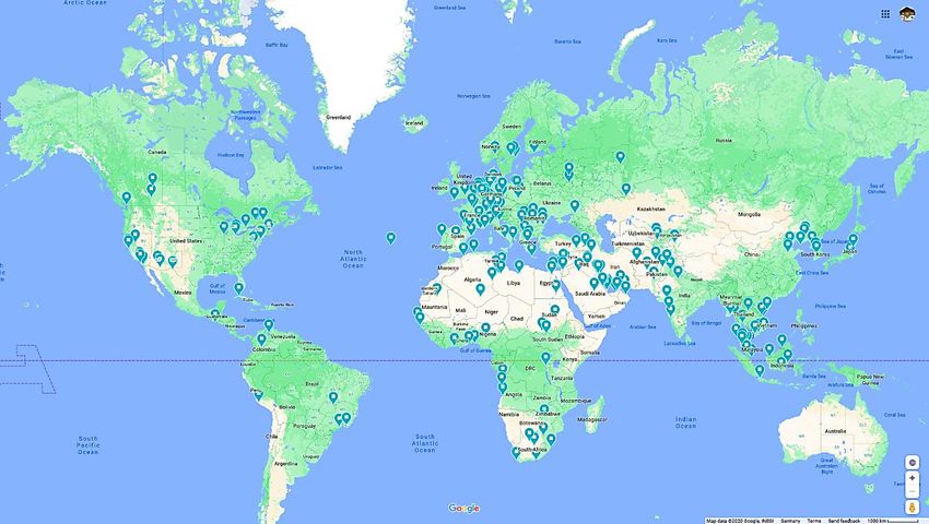
This article has been accepted for publication in a future issue of this journal, but has not been fully edited. Content may change prior to final publication. Citation information: DOI 10.1109/JSTARS.2021.3084314, IEEE Journal
 of Selected Topics in Applied Earth Observations and Remote Sensing
 JSTARS-2021-00425 2

 relations between geographical or architectural areas. Radiometrically Enhanced (RE) data with single polarization
 Conclusions and future research directions that are described in (HH). As product generation option, we took Geo-coded
 Section 6 complete this paper. Appendix II presents the IDs of Ellipsoid Corrected (GEC) data. These images have a pixel
 each selected TerraSAR-X product, and their locations being spacing of 2.5 m and a resolution of 5.75 m. The size of these
 used for analysis, and a benchmark dataset creation, followed few images is 9,885×15,025 pixels (rows × columns). Their
 by Appendix III that displays (for a selected number of incidence angle is 35° and the pass direction is descending.
 TerraSAR-X products from Appendix II) the semantic This dataset covers urban and industrial areas together with
 distribution (in per cent) of each identified label (i.e., semantic their infrastructure from all over the world (data being available
 class or category) in the given images, and its corresponding via [21]). A number of 124 images tiled into 183,412 patches of
 semantic classification map. The last appendix, Appendix IV 160×160 pixels (called Phase I and Phase II) are considered as
 gives a list of semantic classes that are retrieved in our dataset the most interesting target areas. These images are distributed
 with typical examples. over several continents: five scenes from Africa, 35 from Asia,
 54 from Europe, nine from the Middle East, and 21 from North
 II. A SURVEY OF EXISTING SEMANTIC DATASETS and South America. The scenes were selected based on their
 When we compare the retrieval of images or image patches availability, their content, the typical diversity of country-
 from multimedia or remote sensing archives, we can say that specific land cover, and the recording parameters of each scene.
 most multimedia applications aim at the recognition of single At the time of writing, the process of semantic annotation has
 objects in front of mostly irrelevant background, while typical not yet been completed and is one that still will evolve over
 remote sensing applications call for the identification of land time. Another set of 171 images were analyzed with a total of
 cover/land use details or the monitoring of shipping routes 170,145 patches with the same patch size (called Phase III).
 covering the full image area, as well as images of built-up areas These images cover more areas from all over the world (36
 taken with very high resolution. During the last years, we saw scenes from Africa, 32 from Asia, 36 from Europe, 29 from the
 a growing interest in satellite images in order to support a Middle East, and 38 from North and South America). The full
 variety of applications (e.g., change detection, land use list of TerraSAR-X images is detailed in Appendix I, while the
 classification, disaster relief). These remote sensing number of acquisitions is shown in Fig. 1.
 applications are most often using optical datasets, and very few In total, there are about 354,000 patches tiled from the 295
 ones employ SAR datasets. This was our main reason to images (see their geographical location in Fig. 2) and grouped
 compile a reference dataset for SAR image patches, more into 53 independent semantic classes (see Fig. 9, where the
 exactly a high-resolution dataset using TerraSAR-X images [3]. semantic classes are listed with their proportion) without
 Appendix I contains a state-of-the-art survey of existing land deselecting the cases where two semantic classes can be
 cover datasets for space-borne or airborne remote sensing, first assigned to a patch in a multi-labelling approach (e.g., Channels
 for optical sensors, and then for SAR sensors. and High-density residential areas). To these classes we added
 one more class, entitled Unclassified for the patches for which
 III. THE CHARACTERISTICS OF OUR BUILT-FOR-URBAN SAR it was not possible to define a class. This class represents
 DATASET between 1% and (maximum) 10% of the total number of
 patches of an image.
 In this paper, we concentrate on TerraSAR-X, an X-band
 In terms of organization of the proposed SAR reference
 SAR instrument with various operating modes, selectable
 datasets, we opted for our dataset to contain (for each
 polarization, and a number of product generation options [3].
 TerraSAR-X image) the retrieved and semantically labelled
 For most of the investigated areas, we selected High-
 classes with their individual number of patches.
 resolution Spotlight (HS) mode images because they provide a
 In the literature, one can find other datasets that are organized
 lot of details in urban areas. We took horizontally polarized
 differently, e.g., for a defined number of classes where a fixed
 (HH) images as this option is most frequently recorded over
 number of patches are selected from different images. We
 land, and we used images taken from ascending and descending
 believe that this structuring of a dataset is a bit restrictive, and
 pass directions. As for the product generation options, we
 when we eliminate the classes that do not meet the minimum
 selected Multi-look Ground range Detected (MGD) data as they
 number of patches, this does not correspond to the reality in the
 are not affected by geometrical interpolation effects over
 images.
 mountainous terrain and thus are most suited for feature
 extraction [20]. This was also the reason for choosing
 radiometrically enhanced products that are optimized with
 respect to radiometry (i.e., brightness effects). As a result of the
 product mode and product parameter selection, our images have
 a pixel spacing of 1.25 m and a resolution of about 2.9 m. The
 average size of each full scene is 4,200×6,400 pixels (rows ×
 columns). The incidence angle lies between 25° and 48°.
 For two areas (due to the unavailability of some parameters),
 we selected StripMap (SM) mode images, namely
 Fig. 1: Geographical distribution among continents of our analysed images.

 This work is licensed under a Creative Commons Attribution 4.0 License. For more information, see https://creativecommons.org/licenses/by/4.0/

This article has been accepted for publication in a future issue of this journal, but has not been fully edited. Content may change prior to final publication. Citation information: DOI 10.1109/JSTARS.2021.3084314, IEEE Journal
 of Selected Topics in Applied Earth Observations and Remote Sensing
 JSTARS-2021-00425 3

 Fig. 2: Geographical locations of the target areas projected on Google Maps [22].

 generated that was also stored in our database, following the
 IV. A BRIEF DESCRIPTION OF OUR SEMANTIC ANNOTATION hierarchical annotation scheme defined in [1] and using the
 METHODOLOGY ground truth data of Google Earth for a correct assignment of
 the labels.
 The semantic annotation methodology that we developed is The semantic labels were selected based on the content of
 a scheme being used to generate semantic benchmark datasets. each patch; a single label was assigned if more than 50% of the
 This scheme is based on previous work described in [1]; content belonged to a specific class (see the five examples
 however, in this paper the scheme is used to extract the best- shown in Fig. 4). In cases without a clear label, we allocated
 fitting semantic labels. The flow chain was also used to create more semantic labels (see the five examples given in Fig. 5).
 the first semantic catalogue of the TerraSAR-X instrument, a
 work supported by the European Space Agency (ESA) under
 the technology project EOLib (Earth Observation Image
 Librarian) [23].
 Here, we are using the output of the proposed method (see
 the workflow in Fig. 3) in order to efficiently exploit the
 information/knowledge from the semantic labels and to analyse
 the relationships between the different labels identified for each
 observed target area from the dataset.
 A brief description of the methodology (shown in Fig. 3) is
 presented step by step in the following: Create an account (as a
 project proposal for data downloading) in order to have access
 to the TerraSAR-X archives, then select the images that
 correspond to our criteria (in this case, images that cover urban
 areas from all over the world). The images are further tiled into
 patches with a size of 160×160 pixels (in our case, see [20] for
 high-resolution TerraSAR-X images) and we generate a quick-
 look view of each patch and store it in a new database. From
 each patch, its primitive features are extracted, using one of the
 methods described in [20] and stored in the database. By
 applying an active learning (AL) approach based on a Support
 Vector Machine (SVM) with relevance feedback [24], we
 grouped the features following a semi-supervised approach into
 different classes. Up to this stage of the methodology, the steps
 are automated, while for the next steps some user interaction is
 needed.
 After this, we included the classification results of the
 knowledge which was provided by several experts who
 operated the system. For each class, a semantic label was Fig. 3: Proposed methodology to select, classify, semantically label (i.e.,
 annotate) each patch, and generate different results for TerraSAR-X images [1].

 This work is licensed under a Creative Commons Attribution 4.0 License. For more information, see https://creativecommons.org/licenses/by/4.0/

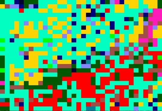
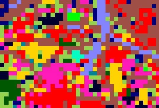
This article has been accepted for publication in a future issue of this journal, but has not been fully edited. Content may change prior to final publication. Citation information: DOI 10.1109/JSTARS.2021.3084314, IEEE Journal
 of Selected Topics in Applied Earth Observations and Remote Sensing
 JSTARS-2021-00425 4

 Once this process had been completed, the benchmark As a result of the proposed approach, Fig. 6 shows for each
 datasets were ready to be used. In addition, each dataset was continent the number of semantic classes being identified, using
 visually inspected by an expert and corrected (if needed). With the scenes from Fig. 1 (see the left pile of the illustration for
 such datasets, we were able to produce semantic classification Phases I and II).
 maps, statistical analytics, classification metrics, etc. See a From the obtained semantics (based on the classification
 number of examples in Appendix III, Table A.III.1 for results and the semantic label assignment by the users), we can
 classification maps, and in Table A.III.2 for statistical analytics. derive several additional results: a) strategies for semantic
 If new types of images (new classes) are to be analysed, we annotation based on the geographical locations of the selected
 have an expert user who is making the semantic annotation of cities; b) statistical analytics based on the retrieved and assigned
 the new images and updates the “Semantic labels database” (by semantics; c) city or country models using the given semantic
 adding the new labels) (see Fig. 3). classes, ontologies, or knowledge graphs.

 Skyscrapers Mixed urban areas Military airplanes Bridges High-density residential areas
 Fig. 4: Five examples of classes with their corresponding sematic labels extracted from a benchmark dataset. Here, each patch is annotated with a single semantic
 label.

 Ploughed agricultural areas Greenhouses and
 Channels and Roads and Roads and Ploughed
 and Low-density residential Ploughed
 Mixed Forest Stubble agricultural land
 areas agricultural land
 Fig. 5: Another five examples of classes with semantic labels extracted from a benchmark dataset. In this figure, the content of each patch is annotated with several
 semantic labels.
 Each column of the matrix refers to a predicted semantic
 class, and the total number of patches in each column represents
 the patches assigned to that class. Each row represents the true
 semantic class, while the total number of patches in each row
 represents the patches of the retrieved class [48].

 Fig. 6: Number of retrieved semantic classes/labels for each continent, based
 on the semantic analysis of the images in Phases I and II from Fig. 1.

 Fig. 7 shows the confusion matrix computed for 12 out of 30
 classes (we had a sufficient number of diverse patches as
 samples). The selected classes are belonging to human-made
 classes and we noticed that they are sometimes mixed up, which
 confirms the “semantic gap” between user-semantic
 1--5 6--10 11--20 21--30 31--40 41--60 61--70 71--80 81--90 91--100 101--110 111--120 121--140
 annotations and computer-semantic predictions that was 141--160 161--180 181--200 201--210 211--220 221--240 241--260 261--280 281--300 301--310 311--320 321--340 341--360
 already pointed out by [47]. 361--380 381--400 401--410 411--420 421--440 441--460 461--480 481--500 501--510 511--520 521--540 541--560 561--580

 Usually, a confusion matrix is used for evaluating the 581--600 601--610 611--620 621--640 641--660 661--680 681--700 701--710 711--720 721--740 741--760 761--780 781--800

 accuracy of the classification. In our case, we computed this Fig. 7: The confusion matrix computed for a number of selected US cities. From
 matrix in order to know more about the accuracy of the the 30 retrieved semantic classes, only the ones linked to human-made
 structures are displayed. In the matrix (upper part), blanks indicate no such
 proposed method using as input data the given TerraSAR-X
 combination. The combinations between classes are marked in different colours
 images. Based on this, we reached an accuracy of between 90% depending on the number of patches (see the legend in the lower part). The
 and 97% depending on the semantic class. values on the diagonal line of the matrix are the highest ones compared to the
 other values on that line (the value from the left or right part of the value on the
 diagonal line).

 This work is licensed under a Creative Commons Attribution 4.0 License. For more information, see https://creativecommons.org/licenses/by/4.0/

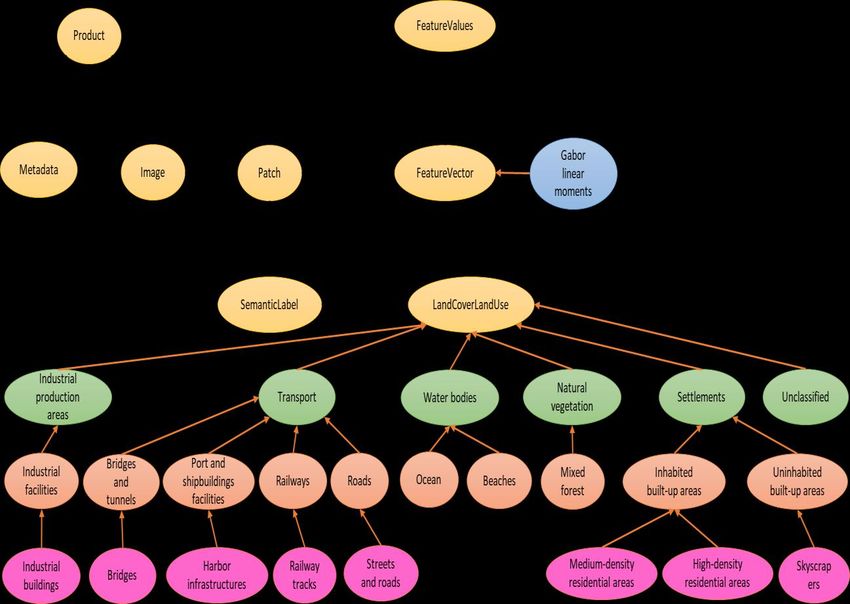
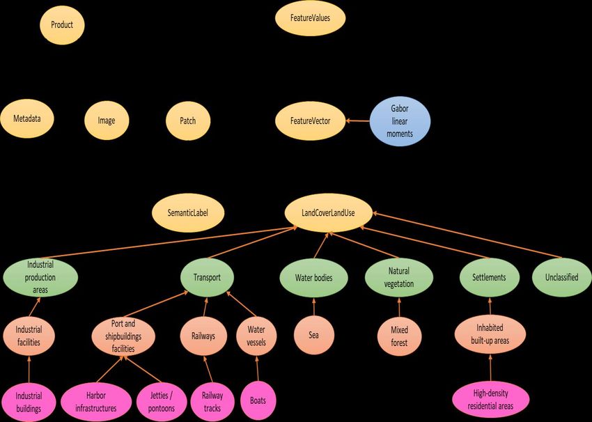
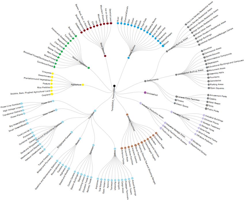
This article has been accepted for publication in a future issue of this journal, but has not been fully edited. Content may change prior to final publication. Citation information: DOI 10.1109/JSTARS.2021.3084314, IEEE Journal
 of Selected Topics in Applied Earth Observations and Remote Sensing
 JSTARS-2021-00425 5

 For example, the value in the seventh column of the seventh semantic classes identified per continent.
 row indicates the number of patches with the label Medium- • Statistics about the surface occupied by urban, industrial,
 density residential areas that belongs to the seventh class being and vegetated areas in a city/country.
 predicted as the seventh class. The value of the seventh row and • A country model based on the retrieved semantic classes.
 the fourth column indicates the number of patches labelled as • An ontology model for high-resolution SAR images.
 Medium-density residential areas that actually belongs to the • Domain ontologies and knowledge-graph
 seventh class being mis-predicted as the fourth class (namely representations.
 High-density residential areas). This principle is applied to all
 columns and lines of the matrix. In our case, we were able to define a nomenclature adapted
 to high-resolution SAR images where we applied a
 Conclusion: Our method is a package of modular components hierarchical semantic annotation scheme with three levels
 to perform the necessary tests. The entire dataset is analysed (see Fig. 8) with a total of 150 classes/categories, of which
 identically by the proposed method using the same patch size nine basic classes (agriculture, forest, hydrology, traffic,
 (160×160 pixels), the same feature extraction method (Gabor building architecture, public use, leisure, mineral/salt, and
 filters with 5 scales and 6 orientations), the same classifier and other land use categories) belong to our level-1, 73 classes
 kernel (SVM with chi-square tests), and the same user belong to level-2, and 68 classes belong to level-3 [1].
 performing the semantic labelling of the retrieved classes Interestingly, the level-3 classes describe details of human-
 (assigning one semantic label per class). The labelled patches made infrastructure, while the categories describing natural
 are stored into a database that is used for further operations environments do not have level-3 refinements. This remark is
 (analytics, ontologies, knowledge graphs, etc.).
 only valid for high-resolution SAR images.
 By applying the procedure from Fig. 3, the entire dataset
 was tiled into about 350,000 patches and each patch was
 V. DISCUSSIONS OF OUR SEMANTIC FINDINGS: STATISTICS,
 labelled with an assumedly correct semantic meaning. In Fig.
 ANALYTICS, MODELS, AND ONTOLOGIES
 9, the semantic labels are grouped into two categories: one
 In this section, we present our nomenclature for semantic that contains 24 semantic labels of human-made structures
 annotation of the retrieved classes using the methodology from (urban labels), and one that contains 30 semantic labels of
 the previous section, followed by an in-depth analysis of the natural environments (non-urban labels). Within the full
 semantics obtained from different points of view: dataset, we identified and annotated 54 independent semantic
 • Criteria to follow in order to semantically annotate classes without considering the case where two or more
 additional images from different target areas. semantic classes can be assigned to a single patch (e.g.,
 • Statistics about the minimum and maximum number of Channels and High-density residential areas).

 SAR
 high-
 resolution

 Fig. 8: Proposed hierarchical semantic annotation scheme with three levels.

 This work is licensed under a Creative Commons Attribution 4.0 License. For more information, see https://creativecommons.org/licenses/by/4.0/

This article has been accepted for publication in a future issue of this journal, but has not been fully edited. Content may change prior to final publication. Citation information: DOI 10.1109/JSTARS.2021.3084314, IEEE Journal
 of Selected Topics in Applied Earth Observations and Remote Sensing
 JSTARS-2021-00425 6

 1) Criteria to follow in order to semantically annotate lower part illustrating the patch classes that are different (and
 additional images from different target areas. cannot be grouped together) or classes that are identical (and
 We also have to discuss which criteria should be grouped are grouped together).
 together with the images. To this end, the full test dataset
 containing hundreds of images was split into separate a) Combining images covering cities from different countries
 collections in order to maximize the number of identifiable In Fig. 10, we grouped together two cities (Toulouse and
 categories, and to semantically annotate them using our Timisoara) belonging to two different countries from Europe
 previous methodology (see Section 4). (France and Romania). These two cities have almost the same
 We mainly focused on differences between the human-made local economic importance with respect to the countries that
 structures (urban and industrial classes), and less on the natural they belong to. We observed that for common classes identified
 environment (with natural and/or vegetation classes) that also in both images (e.g., Low-density residential areas, Medium-
 depend on seasonal effects. density residential areas, and Roads-and-Mixed urban areas),
 their patches cannot be grouped together.
 A similar example is illustrated in Fig. 11, where for two
 cities on the Korean peninsula (Suwon and Pyongyang) we tried
 to group together their classes. In this case, the common classes
 are High-density residential areas, Medium-density residential
 areas, and Low-density residential areas. However, combining
 them together was not possible.
 Another example is shown in Fig. 12, where we analysed the
 African cities of Abuja, Nigeria and Lomé, Togo. The classes
 identified to be the same are Low-density residential areas and
 Pasture-and-Low-density residential areas. Again, combining
 them together was not possible.
 A last example is from the Middle East where the cities of
 Ashdod, Israel and Beirut, Lebanon were analysed. Here,
 following the semantic analysis and the specificity of the cities,
 not a single class was common.
 Similar examples for combining together of cities from
 different countries are: Tashkent, Uzbekistan and Khujand,
 Tajikistan; Belgrade, Serbia and Skopje, Macedonia; Larissa,
 Greece and Djarbakir, Turkey; Lyon, France and Genoa, Italy;
 Baghdad, Iraq and Bandar Imam Khomeini, Iran.

 Fig. 9: Statistical distribution of the semantic labels: (top) the Non-urban
 semantic labels and (bottom) Urban semantic labels identified from our
 TerraSAR-X dataset.

 By grouping, we mean to put together several images and
 then to apply the methodology described in Section 4 (e.g.,
 classification and annotation). The selection of the images to be
 grouped is made by the user. Fig. 13: Percentage of patches for Ashdod, Israel and Beirut, Lebanon. In this
 case there are no identical semantic labels that can be retrieved from the two
 The next figures (Figs. 10-13 and Figs. 15-18) have two cities.
 parts, an upper part which presents the distribution of the
 retrieved semantic classes (given in per cent), followed by a

 This work is licensed under a Creative Commons Attribution 4.0 License. For more information, see https://creativecommons.org/licenses/by/4.0/

This article has been accepted for publication in a future issue of this journal, but has not been fully edited. Content may change prior to final publication. Citation information: DOI 10.1109/JSTARS.2021.3084314, IEEE Journal
 of Selected Topics in Applied Earth Observations and Remote Sensing
 JSTARS-2021-00425 7

 Low-density residential areas-1 Medium-density residential areas-1 Roads-and-Mixed urban areas-1

 Toulouse

 Low-density residential areas-2 Medium-density residential areas-2 Roads-and-Mixed urban areas-2

 Timisoara

 Fig. 10: (top) Percentage of patches for Toulouse, France and Timisoara, Romania. (bottom) In this example, for three labels of Toulouse (first line) and of
 Timisoara (second line) the same semantic labels were assigned: Low-density residential areas, Medium-density residential areas, and Roads-and-Mixed urban
 areas.

 High-density residential areas-1 Medium-density residential areas-1 Low-density residential areas-1

 Suwon

 High-density residential areas-2 Medium-density residential areas-2 Low-density residential areas-2

 Pyongyang

 Fig. 11: (top) Percentage of patches for Suwon, South Korea and Pyongyang, North Korea. (bottom) In this example, for three labels of Suwon (first line) and
 Pyongyang (second line) the same semantics were assigned: High-density residential areas, Medium-density residential areas, and Low-density residential areas.

 This work is licensed under a Creative Commons Attribution 4.0 License. For more information, see https://creativecommons.org/licenses/by/4.0/

This article has been accepted for publication in a future issue of this journal, but has not been fully edited. Content may change prior to final publication. Citation information: DOI 10.1109/JSTARS.2021.3084314, IEEE Journal
 of Selected Topics in Applied Earth Observations and Remote Sensing
 JSTARS-2021-00425 8

 Low-density residential areas-1 Pasture-and-Low-density residential areas-1

 Abuja

 Low-density residential areas-2 Pasture-and-Low-density residential areas-2

 Lomé

 Fig. 12: (top) Percentage of patches for Abuja, Nigeria and Lomé, Togo. (bottom) In this example, for two labels of Abuja (first line) and Lomé (second line) the
 same semantic labels were assigned: Low-density residential areas and Pasture-and-Low-density residential areas.

 Fig. 14: Differences between the cities of Suwon, South Korea and Pyongyang, North Korea for the two labels High-density residential areas (121 patches for
 Suwon and 199 patches for Pyongyang) and Medium-density residential areas (60 patches for Suwon and 40 patches for Pyongyang). Gabor texture filters were
 used to describe the content of each image patch in a set of coefficients. For each patch we computed the means and standard deviations of each coefficient (in
 total, we applied 5 scales × 6 orientations × 2 additional parameters (mean and variance) = 60 coefficients) [1]. Area 1 corresponds to the city of Pyongyang and
 Area 2 corresponds to the city of Suwon. The left plots are generated for the first semantic class, while the right plots are for the second semantic class.

 This work is licensed under a Creative Commons Attribution 4.0 License. For more information, see https://creativecommons.org/licenses/by/4.0/

This article has been accepted for publication in a future issue of this journal, but has not been fully edited. Content may change prior to final publication. Citation information: DOI 10.1109/JSTARS.2021.3084314, IEEE Journal
 of Selected Topics in Applied Earth Observations and Remote Sensing
 JSTARS-2021-00425 9

 from all images. Like in the previous example, there are also
 Conclusion: If the given images depict cities from different other human-made classes that appear in different images (e.g.,
 continents/countries, combining them together leads to High buildings) but not in all four images.
 different semantic classes for the human-made structures. Even A last example is for three cities in Malaysia (see Fig. 17).
 if we have the same semantic class label, the patches cannot be Like in the previous two examples, there are semantic classes
 grouped together due to the different primitive features of the that appear in all three images, and can be grouped together
 two cities (see Fig. 14). (e.g., Medium-density residential areas). As in the case of the
 United Kingdom or U.S.A., there are classes that do not appear
 b) Combining multiple images covering cities belonging to the in all cities (e.g., Skyscrapers).
 same country Similar examples for combining of cities that belong to the
 Here, the combining is performed based on similar source same country are: Canada (Vancouver, Calgary, Ottawa), China
 regions (of the same county). In this case, we mean a similar (Ashan, Binhai, Dalian, Jinan, and Shenyang), France
 geographical location of the cities. (Bordeaux, Lyon, and Toulouse), Greece (Chania, Larissa, and
 A first example is the combining of 12 cities that belong to Thessaloniki), Iran (Bandar Imam Khomeini, Bandar-e-Abbas,
 the United States (see Fig. 15). The selection of the cities is and Mahabad), Italy (Genoa, Naples, Puzzuoli, Taranto, Trento,
 performed to include as much as possible the urban diversity of and Venice), Poland (Bydgoszcz, Czestochowa, Lodz, and
 the country. Based on the results, we noticed that there are Torun), Russia (Krutorozhino, Central, Northern and Southern
 common classes (e.g., High-density residential areas and Moscow, Perm, Rostov on Don, and Tula), etc.
 Medium-density residential areas) that appear in almost 80% of
 the cities, but also human-made classes that appear in two to
 three cities (e.g., Skyscrapers) or only in one city (e.g., Urban Conclusion: If the images cover cities from the same
 houses in residential areas). country, combining them together leads to similar semantic
 A second example is Fig. 16, where the selected four cities classes for the human-made structures. This type of combining
 all belonging to the United Kingdom in Europe. shows us that the geographical location of a city is very
 In this case, one of the common classes selected for important for defining the semantic labels. Even if a semantic
 illustration is Medium-density residential areas that is retrieved class does not appear in all the analysed cities where the
 patches appear, they are grouped together in the same class.

 Ciudad Juarez North part of San Diego Tijuana

 Medium-density residential areas

 High-density residential areas

 Fig. 15: (top) Percentage of patches for twelve US cities: Ciudad Juarez, Los Angeles, North San Diego, South San Diego, Poway, Sun Lakes, Tijuana, Tucson,
 San Francisco, Santa Clarita, Reno, and Washington, DC. In this case, due to the same architecture of the human-made structures, the labels are similar. (bottom)
 We selected three out of twelve cities for which two semantic label names were assigned: High-density residential areas and Medium-density residential areas.

 This work is licensed under a Creative Commons Attribution 4.0 License. For more information, see https://creativecommons.org/licenses/by/4.0/

This article has been accepted for publication in a future issue of this journal, but has not been fully edited. Content may change prior to final publication. Citation information: DOI 10.1109/JSTARS.2021.3084314, IEEE Journal
 of Selected Topics in Applied Earth Observations and Remote Sensing
 JSTARS-2021-00425 10

 First part of Second part of
 London Plymouth
 Portsmouth Portsmouth

 Medium-density residential areas

 Fig. 16: (top) Percentage of patches for four cities from the United Kingdom. In this case, due to the same architecture of the human-made structures, the labels are
 similar. (bottom) In this example we selected all four cities for which one semantic label name was assigned: Medium-density residential areas.

 Alor Setar Seremban Kuala Lumpur

 Medium-density residential areas

 Fig. 17: (top) Percentage of patches for three cities from Malaysia. In this case, due to the same architecture of the human-made structures, the labels are similar.
 (bottom) In this example, we selected all cities for which the same single semantic label name was assigned: Medium-density residential areas.

 This work is licensed under a Creative Commons Attribution 4.0 License. For more information, see https://creativecommons.org/licenses/by/4.0/

This article has been accepted for publication in a future issue of this journal, but has not been fully edited. Content may change prior to final publication. Citation information: DOI 10.1109/JSTARS.2021.3084314, IEEE Journal
 of Selected Topics in Applied Earth Observations and Remote Sensing
 JSTARS-2021-00425 11

 Bremen Karlsruhe Stuttgart Basel

 Medium-density residential areas

 High-density residential areas

 Fig. 18: (top) Percentage of patches for twelve cities from German-speaking countries: Berlin, Bonn, Bremen, Lindau, Karlsruhe, Mannheim, Stuttgart, Cologne,
 Kiel, Oldenburg, Munich, and Basel. In this case, due to the same architecture of the human-made structures, the labels are similar. (bottom) In this example, we
 selected four out of twelve cities for which two semantic label names appeared: High-density residential areas and Medium-density residential areas.

 c) Combining images that cover cities with similar analysed, the maximum (max) and minimum (min) number of
 characteristics but from different countries semantic classes. The maximum number of classes is between
 In this case, the images still belong to cities from the same 18 and 20 for four out of six continents.
 country (e.g., Dharan and Riyad from Saudi Arabia), however, As for the minimum number of semantic classes, the
 the commonly identified human-made structure classes are variation is greater; the upper value is 11 and the lower value is
 separated. This leads us to the conclusion that not only the 4. From the figure, we can see that the overall range is
 geographical source region is important, but also the maintained; a continent with a higher value for max also has a
 architectural characteristics of each city. higher value for min.
 As an example, where the cities are from two different
 countries is presented in Fig. 18. The important characteristics
 of these cities are that they belong to the German-speaking
 countries and have a similar architecture. Based on the results,
 we observed that there are common classes among the cities that
 belong to Germany or Switzerland (e.g., High-density
 residential areas and Medium-density residential areas).

 Conclusion: In this case, due to the same architecture of the
 human-made structures, the classes are similar and the patches
 from different cities are grouped into the same semantic class.

 Fig. 19: Minimum and maximum number of semantic classes/labels per
 2) Statistics about the minimum and maximum number of continent.
 semantic classes identified per continent.
 After the first question, of how to group together a selection
 Conclusion: The minimum and maximum number of semantic
 of images, the second question is how many semantic
 labels of a city depends on the continent where the city belongs
 classes/labels exist in each image.
 to.
 In this context, Fig. 19 gives, for each continent being

 This work is licensed under a Creative Commons Attribution 4.0 License. For more information, see https://creativecommons.org/licenses/by/4.0/

This article has been accepted for publication in a future issue of this journal, but has not been fully edited. Content may change prior to final publication. Citation information: DOI 10.1109/JSTARS.2021.3084314, IEEE Journal
 of Selected Topics in Applied Earth Observations and Remote Sensing
 JSTARS-2021-00425 12

 a metropolitan city for the region to which it belongs to.
 3) Statistics about the surface occupied by urban, industrial, From the total number of annotated patches, 41% can be
 and vegetated areas in a city/country grouped into the class of High-density residential areas to
 Here we analysed each city from three points of view based which we added another 3% of patches that are grouped
 on the semantic classes obtained when applying the into Medium-density residential areas.
 methodology described in Section 4. • The selected Italian city is Naples. From Fig. 20 (second
 line on the left), we recognize that this city is the one with
 a) How developed is an urban area? the highest number of patches semantically recognized as
 In order to answer this question, we investigated for each city High-density residential areas, when compared with the
 the semantic classes that belong to Settlements (see Fig. 8). By other five Italian cities from the same figure. This class is
 analysing the existence of semantics such as Skyscrapers, High the one with the highest percentage (of 17%) from all
 buildings, or High-density residential areas we can say that this annotated patches, except for the class Sea which obtains
 city is a metropolitan city, a financial center or even the capital 66%. When analysing the demographic statistics (in Table
 of a country. In the opposite case, when the resulting semantics 1), we see that Naples is a city with a big population and
 are Very low-density residential areas, or Low-density population density.
 residential areas that city is a smaller city, such as a provincial Venice is the city ranking next to Naples where the class
 city. High-density residential areas contains less patches
 In Fig. 20, the semantic classes that are the most common annotated with this label (the percentage with respect to
 urban ones (Very low-density residential areas, Low-density all annotated patches is 13%).
 residential areas, Medium-density residential areas, High- • The selected Russian city is Moscow where we analysed
 density residential areas, Mixed urban areas, High buildings, three parts of it: Center, South, and North. From the
 and Skyscrapers) were derived from images of four countries. semantical analysis in Fig. 20 (second line on the right),
 We analysed: in case of China five cities, in case of Germany we got 25% of the patches grouped as High buildings,
 eleven cities, in case of Russia five cities, and in case of the 30% of the patches grouped as High-density residential
 U.S.A. ten cities. Note that we collected the patches with areas, and 20% of the patches grouped as Medium-density
 semantic labels that are in relation to urban areas and the residential areas. Based on these results and strengthened
 remaining patches that are not belonging to this classes are by demographic statistics (in Table 1), we can state that
 grouped into other classes such as Industrial production areas, this city is the largest metropolitan city (see also
 Transport, Agriculture, Natural vegetation, Bare ground, Wikipedia description “Moscow is the capital and largest
 Water bodies, or Unclassified. city of Russia and the largest metropolitan area in
 In Table 1, we collected from Wikipedia some information Europe”).
 about the population living in each given city, the surface of the • The selected US city is San Francisco with the biggest
 city, and its population density [43]. When we analysed each population density per km2 among the given US cities (see
 city based on its retrieved semantic classes (obtained based on Table 1). When analysing the retrieved semantic classes
 our approach from Section 4), we correlated the observations shown in Fig. 20 (center of lowermost graphics), we can
 with the data collected from Wikipedia for each city. say that this is a metropolitan city with prominent classes
 In the following, we are investigating in detail, based on the like Skyscrapers (11% of all annotated patches) and High-
 semantics but also considering important demographic data, the density residential areas (53%). This result is in line with
 most important cities (one per country) from our dataset and current demographic statistics.
 from Fig. 20. The Chinese cities are the ones with seven
 semantic classes (as upper value) in opposition to Italian cities b) How industrialized is a city?
 that have only three semantic classes (as upper value). To answer this question, we had to compare the semantic
 • The selected Chinese city is Shenyang (the one with the labels Built-up areas with Industrial areas. This comparison
 biggest population). When analysing the retrieved was made for the same cities and countries like in Fig. 20. From
 semantics shown in Fig. 20 (first line on the left), we can this we can see how industrialized is a city/country compared
 say that this city is a metropolitan city with the typical to another city/country. By analysing each city one by one in
 classes Skyscrapers (10% of all annotated patches), High- Fig. 21, we can state the following:
 density residential areas (23%) but also Medium-density • The most industrialized cities (from the ones available in
 residential areas (13%). This observation is also our dataset) are Binhai, China; Mannheim, Germany;
 reinforced by the demographic statistics (see Table 1) Pozzuoli, Italy; Krutorozhino, Russia; and Tucson, U.S.A.
 which show that this city is a very populated one. • The least industrialized cities (from the ones available in
 • The selected German city is Munich. This is the third- our dataset) are Shenyang, China; Munich, Germany;
 ranking city with a big population and density (see Table Naples, Italy; Center of Moscow, Russia; San Francisco,
 1). When analysing the retrieved semantic classes U.S.A.
 illustrated in Fig. 20 (first line on the right), we notice that
 this city is an important city. We can even say that this is

 This work is licensed under a Creative Commons Attribution 4.0 License. For more information, see https://creativecommons.org/licenses/by/4.0/

This article has been accepted for publication in a future issue of this journal, but has not been fully edited. Content may change prior to final publication. Citation information: DOI 10.1109/JSTARS.2021.3084314, IEEE Journal
 of Selected Topics in Applied Earth Observations and Remote Sensing
 JSTARS-2021-00425 13

 Fig. 20: Statistical distribution of the semantic class Inhabited built-up areas for China, Germany, Italy, Russia, and the U.S.A. The vertical axis describes the
 number of patches that are semantically annotated with this label for each city.

 Lindau 25,512 33 770
 Mannheim 310,658 145 2,100
 TABLE I Munich 1,484,226 311 2,606
 THE SURFACE COVERED BY EACH SELECTED CITY, THE POPULATION LIVING IN
 Oldenburg 169,077 103 1,600
 THE CITY, AND DENSITY OF INHABITANTS PER KM2.
 Stuttgart 635,911 207 3,100
 Inhabitants
 City Population Area in km2 Genoa 580,097 240 2,400
 per km2
 Naples 967,068 119 8,100
 Anshan 1,406,000 9,252 390
 Pozzuoli 80,074 Not available Not available
 Italy

 Binhai 1,000,000 2,270 440
 China

 Taranto 198,585 250 790
 Dalian 4,009,700 12,574 532
 Trento 118,160 158 750
 Jinan 4,693,700 7,171 850
 Venice 260,897 415 630
 Shenyang 5,119,100 12,942 640
 Not
 Berlin 3,669,491 892 3,944 Krutorozhino Not available Not available
 available
 Bonn 329,673 141 2,300 Moscow 12,506,468 2,511 Not available
 Germany

 Russia

 Bremen 567,559 327 1,700 Perm 991,162 800 1,200
 Cologne 1,087,863 405 2,700 Rostov on
 1,089,261 349 3,100
 Karlsruhe 312.06 174 1,800 Don
 Kiel 246,794 119 2,100 Tula 501,169 154 3,300

 This work is licensed under a Creative Commons Attribution 4.0 License. For more information, see https://creativecommons.org/licenses/by/4.0/

This article has been accepted for publication in a future issue of this journal, but has not been fully edited. Content may change prior to final publication. Citation information: DOI 10.1109/JSTARS.2021.3084314, IEEE Journal
 of Selected Topics in Applied Earth Observations and Remote Sensing
 JSTARS-2021-00425 14

 Los Angeles 3,979,576 1,302 3,276
 San Diego 1,307,402 965 1,687
 Poway 47,811 102 487
 Reno 47,811 289 907
 San
 U.S.A.

 881,549 601 7,255
 Francisco
 Santa Clarita 176,320 184 1,162
 Sun Lakes 13,975 14 Not available
 Tijuana 1,902,385 637 Not available
 Tucson 520,116 624 880
 Washington Fig. 21: Number of patches retrieved as Inhabited built-up areas versus
 6,133,552 3,644 419
 DC Industrial production areas. These plots consider five cities in China, eleven
 cities in Germany, six cities in Italy, five cities in Russia, and ten cities in the
 U.S.A.

 c) How green is the city?
 In order to answer this last question, we needed to compare
 the vegetated areas with the urban built-up areas. This was done
 by analysing the semantic classes that include vegetation versus
 the semantic classes that include urban classes.
 Analysing Fig. 22, we can say that for all continents the area
 occupied by inhabited built-up classes is larger than the area
 occupied by natural vegetation. Further details are described in
 the following list:
 • Africa (in this example, the city of Port Elizabeth, South
 Africa): the percentage of the area occupied by vegetation
 is close to the one occupied by the urban built-up area.
 • Asia (in this case, the city of Tokyo, Japan): the
 percentage of the area occupied by vegetation is very
 small compared with the one occupied by the urban area.
 • Europe (in this example the city of Porto, Portugal): the
 percentage of the area occupied by vegetation is about
 three times less than the one occupied by the urban area.
 • Middle East (in this case the city of Ashdod, Israel): the
 percentage occupied by vegetation is the lowest of all
 cases, because this region is one with a lot of desert/sand.
 • North America (in this case the city of Ottawa, Canada):
 the vegetation percentage is about 10% of the urban area.
 • Central and South America (in this case the city of
 Havana, Cuba): the percentages of vegetation and urban
 classes are close to each other.

 Fig. 22: A comparison between the urban area (Inhabited built-up areas) and
 the vegetated area (Natural vegetation) for one city per continent. A percentage
 difference of up to 100% is occupied by other classes (e.g., Water bodies).

 This work is licensed under a Creative Commons Attribution 4.0 License. For more information, see https://creativecommons.org/licenses/by/4.0/

This article has been accepted for publication in a future issue of this journal, but has not been fully edited. Content may change prior to final publication. Citation information: DOI 10.1109/JSTARS.2021.3084314, IEEE Journal
 of Selected Topics in Applied Earth Observations and Remote Sensing
 JSTARS-2021-00425 15

 Conclusion: Such statistics is very useful for municipalities,
 for those being engaged in the urbanism of the city but also for
 potential real-estate investors. The results can be correlated
 with other statistics gathered by local/government
 administrations (e.g., population censuses, demographic and
 economic statistics).

 4) A country model based on the retrieved semantic classes
 To create a country and/or a city model, we propose two
 strategies:

 a) Our first strategy considers for each country being
 investigated all the corresponding cities (select the country
 with a high number of analysed cities) and the identified
 semantic classes that belong to urban areas (e.g., Inhabited
 built-up areas) plus the semantic classes that belong to the
 industrial area (e.g., Industrial facilities).
 In this strategy, we do not consider the natural classes
 such as: Agriculture, Natural vegetation, Bare ground, and
 Water bodies.
 Here, the analysed countries with their corresponding
 cities are: China with Anshan, Binhai, Dalian, Jinan, and
 Shenyang; Germany with Berlin, Bonn, Bremen, Cologne,
 Karlsruhe, Kiel, Lindau, Mannheim, Munich, Oldenburg,
 and Stuttgart; Italy with Genoa, Naples, Pozzuoli, Taranto,
 Trento, and Venice; Russia with Krutorozhino, Moscow,
 Perm, Rostov on Don, and Tula; the U.S.A. with Los
 Angeles, San Diego, Poway, Reno, San Francisco, Santa
 Clarita, Sun Lakes, Tijuana, Tucson, and Washington DC.
 Following this strategy, Fig. 23 depicts for each
 individual country the corresponding model results based on
 the retrieved semantic classes of each city (using the
 classification and annotation strategy from Section 4). For
 each city, the semantic classes having been analysed are:
 Skyscrapers, High buildings, High-density residential
 areas, Medium-density residential areas, Low-density
 residential areas, Very low-density residential areas, Mixed
 urban areas, Urban houses in residential areas, and
 Industrial facilities.
 Finally, Fig. 23 shows for each country a model (see the
 average line); these models are further compared in Fig. 24
 with respect to urban classes, and urban and industrial
 classes.
 Analysing the illustrations from Fig. 23, we can say that
 for the U.S.A. and China the country model contains the
 Skyscrapers class that does not appear in the other three
 countries. In opposition to this class, the High buildings
 class, which is very close to Skyscrapers is found in
 Germany and Russia.
 The differences between these country models appear
 especially in the case of urban classes of the following
 categories: High-density residential areas, Medium-density
 residential areas, Low-density residential areas, and Mixed
 urban areas plus the industrial classes (e.g., Industrial
 Fig. 23: A model for five countries (e.g., China, Germany, Italy Russia, and the
 facilities). U.S.A.) comparing the urban and industrial semantic classes retrieved for each
 city of the respective country.

 This work is licensed under a Creative Commons Attribution 4.0 License. For more information, see https://creativecommons.org/licenses/by/4.0/

This article has been accepted for publication in a future issue of this journal, but has not been fully edited. Content may change prior to final publication. Citation information: DOI 10.1109/JSTARS.2021.3084314, IEEE Journal
 of Selected Topics in Applied Earth Observations and Remote Sensing
 JSTARS-2021-00425 16

 The magnitude-shape characteristics of this model creation of the semantic model of the country is shown in
 depends on the retrieved classes which are defined by the Fig. 27 (bottom).
 number of patches belonging to these semantic classes for The last model (see Fig. 28 (top)) is for Middle Eastern
 each city being analysed. countries with a total of seven cities from four countries.
 A more intuitive comparison, preserving the proportions Their distribution per country is the following one: three
 of each model, is presented in Fig. 24. cities from Iran, two cities from Saudi Arabia, one city from
 Lebanon, and one city from Israel. In Fig. 28 (bottom), we
 show the weight (in percent) of each semantic class which
 has an impact when compiling the model.
 Finally, Fig. 29 puts together all the models created for
 each continent and the countries belonging to it.
 The Asian classes that these countries/cities have in
 common are: Channels, High-density residential areas,
 Industrial buildings, Medium-density residential areas,
 Mixed forest, Mixed urban areas, Railway tracks, Roads,
 and Stubble.
 The North American classes that these countries/cities
 have in common are: Boats, Bridges, Channels, High-
 density residential areas, Industrial buildings, Medium-
 density residential areas, Mixed forest, Ocean, Ploughed
 agricultural land, Port facilities, Railway tracks, Roads,
 Skyscrapers, Sparse trees, Sports grounds, Storage tanks,
 and Stubble.
 The European classes that these countries/cities have in
 common are: Bridges, Channels, High buildings, High-
 density residential areas, Industrial buildings, Low-density
 residential areas, Medium-density residential areas, Mixed
 forest, Ploughed agricultural land, Railway tracks, Rivers,
 Roads, Sports grounds, and Stubble.
 Fig. 24: Comparative model extracted from Fig. 23 for the five selected The Mid-Eastern classes that these countries/cities have
 countries. (left) Considering only the urban classes and (right) Considering not in common are: Airport buildings, Industrial buildings,
 only the urban classes but also the industrial ones.
 Medium-density residential areas, Roads, and Sand.
 The other classes (that are not common), are the classes
 b) Our second strategy considers more countries/cities when that are specific to each city/country/continent and we can
 the model is created. This strategy takes into account all the outline the specificity of each of them.
 53 semantic classes having been identified (except for the For example, below we are listing some classes that are
 Unclassified class) after semantically annotating the entire specific to cities/countries/continents:
 dataset.
 • Sand is a semantic class that is specific to the Middle
 In Fig. 25 (top), the models are created for four countries
 East. Here, we are not referring to sand on a beach.
 belonging to the Asian continent, and a total of 18 cities are
 • Skyscrapers is a semantic class that is mainly visible
 analysed. For China there are five cities, for India there are
 in North America and Asia.
 three cities, for Malaysia there are three cities, and for
 • Chemical plants is a class specific to oil extraction
 Russia there are seven cities. In Fig. 25 (bottom), we present
 areas (e.g., Iran) but also in highly-industrialized
 for the same countries the weight (as a percentage) of each
 countries (e.g., China).
 semantic class that provides a contribution to the model of
 the respective country. • Rice paddies is a class specific to Asian countries
 In Fig. 26 (top), the models are created for 15 cities that (e.g., China, India, Indonesia) [29].
 belong to two North American countries. For the U.S.A., we • Exotic trees is a class identified in Greece but also in
 analysed 12 cities, while for Canada three cities. Similarly other Mediterranean countries.
 to the previous figure, Fig. 26 (bottom) presents the • Vineyards is a class identified in the
 percentage of each class that enters the model creation. regions/countries that are big wine producers.
 In the next pictures, Fig. 27 (top) illustrates the role of six Among them we would like to mention: Puglia, Italy;
 European countries with a total of 27 cities. The countries Bordeaux, France; Porto, Portugal; and Rioja, Spain.
 are selected to show off their diversity all over Europe. For
 France we used three cities, for Germany 11 cities, for Italy
 six cities, for Poland three cities, and for the UK four cities.
 The percentage of each semantic class which enters into the

 This work is licensed under a Creative Commons Attribution 4.0 License. For more information, see https://creativecommons.org/licenses/by/4.0/