Quantifying floodwater impacts on a lake water budget via volume-dependent transient stable isotope mass balance - HESS
←
→
Page content transcription
If your browser does not render page correctly, please read the page content below
Hydrol. Earth Syst. Sci., 25, 3731–3757, 2021
https://doi.org/10.5194/hess-25-3731-2021
© Author(s) 2021. This work is distributed under
the Creative Commons Attribution 4.0 License.

Quantifying floodwater impacts on a lake water budget via
volume-dependent transient stable isotope mass balance
Janie Masse-Dufresne1 , Florent Barbecot2 , Paul Baudron1 , and John Gibson3,4
1 Department of Civil, Geological, and Mining Engineering, Polytechnique Montréal, Montreal, QC H3T 1J4, Canada
2 Department of Earth and Atmospheric Sciences, Geotop-UQAM, Montreal, QC H2X 3Y7, Canada
3 InnoTech Alberta, 3-4476 Markham Street, Victoria, BC V8Z 7X8, Canada
4 Department of Geography, University of Victoria, Victoria, BC V8W 3R4, Canada

Correspondence: Janie Masse-Dufresne (janie.masse-dufresne@polymtl.ca)

Received: 2 March 2020 – Discussion started: 16 April 2020
Revised: 27 May 2021 – Accepted: 4 June 2021 – Published: 1 July 2021

Abstract. Isotope mass balance models have undergone sig-         to inform, understand, and predict future water quality vari-
nificant developments in the last decade, demonstrating their     ations. From a global perspective, this knowledge is use-
utility for assessing the spatial and temporal variability in     ful for establishing regional-scale management strategies for
hydrological processes and revealing significant value for        maintaining water quality at flood-affected lakes, for predict-
baseline assessment in remote and/or flood-affected settings      ing the response of artificial recharge systems in such set-
where direct measurement of surface water fluxes to lakes         tings, and for mitigating impacts due to land use and climate
(i.e. stream gauging) are difficult to perform. In this study,    changes.
we demonstrate that isotopic mass balance modelling can be
used to provide evidence of the relative importance of di-
rect floodwater inputs and temporary subsurface storage of
floodwater at ungauged lake systems. A volume-dependent           1   Introduction
transient isotopic mass balance model was developed for an
artificial lake (named lake A) in southern Quebec (Canada).       Lakes are complex ecosystems which play a valuable eco-
This lake typically receives substantial floodwater inputs dur-   nomic, social, and environmental role within watersheds
ing the spring freshet period as an ephemeral hydraulic con-      (Kløve et al., 2011). In fact, lacustrine ecosystems can pro-
nection with a 150 000 km2 large watershed is established.        vide a number of ecosystem services, such as biodiversity,
First-order water flux estimates to lake A allow for impacts      water supply, recreation and tourism, fisheries, and seques-
of floodwater inputs to be highlighted within the annual wa-      tration of nutrients (Schallenberg et al., 2013). The actual
ter budget. The isotopic mass balance model has revealed that     benefits that can be provided by lakes depend on the wa-
groundwater and surface water inputs account for 60 %–71 %        ter quality, and poor resilience to water quality changes can
and 39 %–28 % of the total annual water inputs to lake A,         lead to benefit losses (Mueller et al., 2016). Globally, the
respectively, which demonstrates an inherent dependence of        quantity and quality of groundwater and surface water re-
the lake on groundwater. However, when considering the po-        sources are known to be affected by land use (Baudron et
tential temporary subsurface storage of floodwater, the parti-    al., 2013; Cunha et al., 2016; Lerner and Harris, 2009; Scan-
tioning between groundwater and surface water inputs tends        lon et al., 2005) and climate changes (Delpla et al., 2009).
to equalize, and the lake A water budget is found to be more      As both surface water and groundwater contribute to lake
resilient to groundwater quantity and quality changes. Our        water balances (Rosenberry et al., 2015), changes that af-
findings suggest not only that floodwater fluxes to lake A        fect the surface water/groundwater apportionment can po-
have an impact on its dynamics during springtime but also         tentially modify or threaten lake water quality (Jeppesen et
significantly influence its long-term water balance and help      al., 2014). Understanding hydrological processes in lakes can
                                                                  help to depict the vulnerability and/or resilience of a lake

Published by Copernicus Publications on behalf of the European Geosciences Union.
3732                                      J. Masse-Dufresne et al.: Quantifying floodwater impacts on a lake water budget

to pollution (Rosen, 2015) and to invasive species (Walsh et      ability when conducting lake water budget studies. Our ap-
al., 2016) and, thus, secure water quantity and quality over      proach builds on that of Zimmermann (1979) and Petermann
time for drinking water production purposes (Herczeg et al.,      et al. (2018), developing a predictive model of both atmo-
2003). In Quebec (Canada), there are an important number of       spheric and water balance controls on isotopic enrichment
municipal wells that receive contributions from surface wa-       and accounting for volumetric changes on a daily time step.
ter resources (i.e. lakes or rivers) and are, thus, performing       The main objective of this study is to provide evidence
unintentional (Patenaude et al., 2020) or intentional (Masse-     of the relative importance of direct floodwater inputs and
Dufresne et al., 2019, 2021) bank filtration.                     temporary subsurface storage of floodwater at ungauged lake
    Over the past few decades, significant developments have      systems using an isotopic mass balance model. To do so, we
been made in the application of isotope mass balance mod-         first aim to establish an isotopic framework based on the lo-
els for assessing the spatial and temporal variability in hy-     cal water cycle, to verify the applicability of isotopic mass
drological processes in lakes, most notably the quantification    balance in the present setting, as contrasting isotopic sig-
of groundwater and evaporative fluxes (Herczeg et al., 2003;      natures are required between various water reservoirs and
Bocanegra et al., 2013; Gibson et al., 2016; Arnoux et al.,       fluxes, including floodwater inputs. Second, we quantify the
2017b). In remote environments, such as in northern Canada,       water budget according to two reference scenarios (A and B)
the application of isotopic methods is particularly convenient    to grasp the impact of site-specific uncertainties on the com-
as direct measurements of surface water and groundwater           puted results. Then, we analyse the temporal variability in
fluxes is time-consuming, expensive, and difficult (Welch et      the groundwater inputs and the sensitivity of the lake to
al., 2018). Isotopic mass balance models can notably be ap-       floodwater-driven pollution. Finally, we demonstrate the im-
plied to ungauged lake systems to efficiently characterize the    plications of floodwater-like subsurface inputs on the water
impacts of floods on water apportionment (Haig et al., 2020).     balance partition.
While isotopic frameworks were successfully used to assess           The water balance is computed via a volume-dependent
the relative importance of floodwater inputs to lakes (Turner     transient isotopic mass balance model, which is applied to
et al., 2010; Brock et al., 2007), no attempt was made to eval-   predict the daily isotopic response of an artificial lake in
uate the timing of the floodwater inputs and to differentiate     Canada that is ephemerally connected to a 150 000 km2 wa-
between the role of (i) direct floodwater inputs and (ii) tem-    tershed during spring freshet. During these flood events, the
porary subsurface storage of floodwater on a lake’s annual        surficial water fluxes entering the study lake are not con-
water budget. In this study, direct inputs refer to the flood-    strained in a gaugeable river or canal but occur over a 1 km
water that enters a lake via the surface (e.g. by inundating      wide surficial flood area. Our study period spans a flood with
and/or flowing through a stream), while temporary subsur-         an average recurrence interval of 100 years and is therefore
face storage of floodwater encompasses the floodwater-like        an example of the response of the system to a major hydro-
inputs that reach the lake via the subsurface (e.g. through       logical event.
floodplain recharge or bank storage).
    To gain information on the timing of hydrological pro-
cesses, one may use a transient and short time step isotopic      2     Study site
mass balance. A previous study by Zimmermann (1979) used
                                                                  2.1    Geological and hydrological settings
a transient isotope balance to estimate groundwater inflow
and outflow, evaporation, and residence times for two young       The study site is located in the area of Greater Montreal
artificial groundwater lakes near Heidelberg, Germany, al-        and borders the lake Deux Montagnes (further referred to as
though these lakes had no surface water connections, and          lake DM), which corresponds to a widening of the Ottawa
volumetric changes were considered negligible. Zimmer-            River at the confluence with the St Lawrence River in Que-
mann (1979) showed that the lakes were actively exchang-          bec (Canada; Fig. 1). The Ottawa River is the second-largest
ing with groundwater, which controlled the long-term rate         river in eastern Canada, draining a watershed of approxi-
of isotopic enrichment to isotopic steady state, but the lakes    mately 150 000 km2 (MDDELCC, 2015). The water level
also responded to seasonal cycling in the magnitude of wa-        of lake DM is partly controlled by flow regulation struc-
ter balance processes. While these findings are informative,      tures (e.g. hydroelectric dams) upstream on the Ottawa River.
Zimmermann (1979) did not attempt to build a predictive iso-      Lake DM water levels also show seasonal fluctuations in re-
tope mass balance model but rather used a best-fit approach       sponse to precipitation and snowpack melting over the Ot-
to obtain a solitary long-term estimate of water balance par-     tawa River watershed. High water levels at lake DM are
titioning for each lake. Petermann et al. (2018) also con-        typically observed during springtime (April–May) and, less
strained groundwater connectivity for an artificial lake near     prominently, during autumn (November–December), while
Leipzig, Germany, with no surface inlet or outlet. By com-        lowest water levels normally occur at the end of the summer
paring groundwater inflow rates obtained via stable isotope       (September; Centre d’expertise hydrique du Québec, 2020).
and radon mass balances on a monthly time step, Petermann
et al. (2018) highlighted the need to consider seasonal vari-

Hydrol. Earth Syst. Sci., 25, 3731–3757, 2021                                        https://doi.org/10.5194/hess-25-3731-2021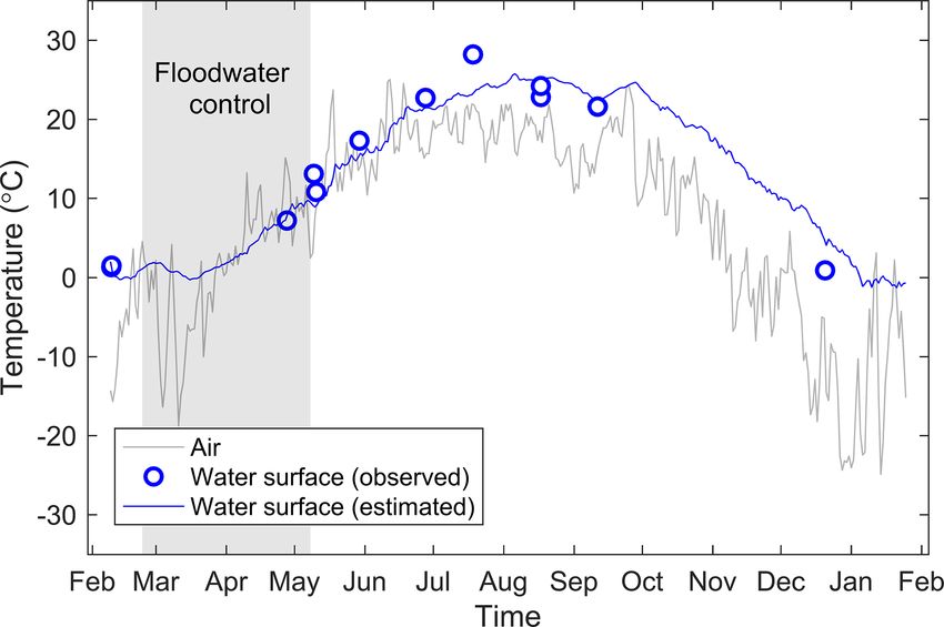
J. Masse-Dufresne et al.: Quantifying floodwater impacts on a lake water budget                                                        3733

Figure 1. (a–c) Location of the study site, relative to the Ottawa River watershed, lake Deux Montagnes (DM), and the area of Greater
Montreal. (d) Location of lake A and lake B relative to lake DM and a schematic representation of the hydrogeological context. The grey
dashed lines illustrate the approximative extent of the paleo valley. LA-S1 and LB-S1 are surface water sampling points at lake A and lake B,
respectively. LA-P1 to LA-P4 correspond to vertical profile sampling locations at lake A. The maps were created from openly available data
and used in accordance with the Open Government Licence – Canada, or the Open Data Policy, M-13-13 of the United States Census Bureau.
Detailed source information is provided in Appendix A.

   Lake A (2.79 × 10⁵ m2 ) and lake B (7.6 × 10⁴ m2 ) are two               Lake A is connected to a small stream (S1) with a mean
small artificial lakes created from sand-dredging activities             and maximum annual discharge of 0.32 and 1.19 m3 s−1 , re-
and are located at approximately 1 km from the shore of                  spectively (Ageos, 2010). Maximum discharge typically oc-
lake DM. The dredging is still ongoing at lake A, while it               curs during the month of April as S1 drains snowmelt wa-
ceased a few decades ago at lake B. Both lakes are approx-               ter from a small watershed (14.4 km2 ; Centre d’expertise hy-
imately 20 m deep (Masse-Dufresne et al., 2019) and were                 drique du Québec, 2019), whereas low flow is recorded for
excavated within alluvial sands which were deposited in a pa-            the rest of the hydrological year. For the springtime in 2017,
leo valley extending in the NE–SW direction and carved into              the surface water flows from S1 are deemed negligible com-
the Champlain Sea clays (Ageos, 2010). Lithostratigraphic                pared to the floodwater inputs and are thus not considered in
data (i.e. well logs) suggest that the paleo valley is approxi-          this study.
mately 600 m wide and has a maximum depth of 25 m. Be-                      In total, two channelized outlet streams (S2 and S3) allow
tween lake DM and lake A, a thin layer (few centimetres to               water to exit lake A and flow towards lake DM. The direc-
roughly 2 m) of alluvial sands are deposited on top the clayey           tion of the surface water fluxes at S2 can be reversed if wa-
sediments (Fig. S1 in the Supplement; Ageos, 2010).                      ter level at lake DM exceeds both a topographic threshold

https://doi.org/10.5194/hess-25-3731-2021                                              Hydrol. Earth Syst. Sci., 25, 3731–3757, 2021
3734                                        J. Masse-Dufresne et al.: Quantifying floodwater impacts on a lake water budget

                                                                     lar pattern from late February to late July 2017 (R 2 = 0.93
                                                                     and p value < 0.01). Considering the above and a visible hy-
                                                                     draulic connection between the lake DM and lake A, the data
                                                                     indicate that the daily water level variations at observation
                                                                     well VP were controlled by lake DM from late February to
                                                                     late July 2017. The lake A water level was also presumably
                                                                     controlled by lake DM until late July 2017, but technical is-
                                                                     sues prevented confirmation (i.e. the logger in lake A broke
                                                                     on 17 May 2017).
                                                                        Then, from August to late October 2017, the water level
                                                                     in lake DM was below the topographical threshold, and
                                                                     there is no similarity between the evolution of the water
Figure 2. Daily mean water levels at lake A, lake DM, and obser-
                                                                     level at lake DM and observation well VP (R 2 = 0.11 and
vation well VP from 9 February 2017 to 25 January 2018. The grey
shaded area corresponds to the floodwater control period. Qmax and
                                                                     p value > 0.01). It is, thus, possible to infer that the lake A
Qmin indicate the timing of the adjusted maximum and minimum         water level was not controlled by lake DM from August to
output from the lake.                                                late October 2017. This is also supported by the manual mea-
                                                                     surement of the lake A water level in September.
                                                                        The water level of lake DM exceeded the topographic
at 22.12 m a.s.l. (above sea level; determined from a topo-          threshold again from November 2017 to January 2018,
graphic land survey along S2) and the water level at lake A          but the daily mean water levels at lake DM and observa-
(Ageos, 2010). Flow reversal also occurs in S3, but the ele-         tion well VP show a moderate correlation (R 2 = 0.63 and
vation of the topographic threshold is unknown.                      p value < 0.01). The manual measurements also indicate a
   Lake A and lake B both contribute to the supply of a              discrepancy between lake DM and lake A water levels in De-
bank filtration system which is composed of eight wells and          cember 2017 and January 2018. The weaker correlation be-
is designed to supply drinking water for up to 18 000 peo-           tween the water level measurements suggests that lake DM
ple (Ageos, 2010). Typically, two to three wells are oper-           was not controlling the dynamics of the lake A water level. It
ated on a daily basis at a total pumping rate ranging from           is, thus, likely that lake A received little to no surface water
4000 m3 d−1 (in wintertime) to 7500 m3 d−1 (in summer-               inputs from lake DM from November 2017 to January 2018.
time; Masse-Dufresne et al., 2019). Although the operation           In this context, surface water inflows from lake DM during
of the bank filtration system does not form a complete hy-           autumn and winter are considered negligible in this study and
draulic barrier between the two artificial lakes, it does lead to    not included in the developed stable isotope mass balance
a lowering of the lake B water level to below that of lake A         model (Sect. 4.2).
(Ageos, 2010).
                                                                     2.3   Conceptual model of lake A water balance
2.2    Hydrodynamics of the major flood event
                                                                     Based on the geological and hydrological setting of the study
In 2017, a major flood event occurred in the peri-urban re-          site (Sect. 2.1) and flood-specific considerations (Sect. 2.2),
gion of Montreal and was caused by the combination of                we established a conceptual model of the lake A water bal-
intense precipitation and snowpack melting over the Ot-              ance, as described below.
tawa River watershed (Teufel et al., 2019). Rapid water                 Considering that lake A is sitting in alluvial sands (i.e. a
level rise at lake DM occurred in late February, early April,        highly permeable material), it is assumed that groundwater
and early May at rates of approximately 0.11, 0.19, and              inputs (IG ) and outputs (QG ) contribute to the water budget.
0.16 m d−1 , respectively. A historical maximum water level          Although it is difficult to interpret the location of IG , it ap-
(i.e. 24.77 m a.s.l.) was reached on 8 May 2017, correspond-         pears evident that QG occur along the NE bank of lake A.
ing to a net water level rise of > 2.7 m compared to early           In fact, there are subsurface fluxes across the sandy bank
February (Fig. 2). High water levels at lake DM resulted             that contribute to the bank filtration system or discharge into
in the inundation of the area between lake A and lake DM             lake B, as its water level has been lower since the initia-
(Fig. 1d), and the surface water fluxes were not constrained         tion of the bank filtration system (Masse-Dufresne et al.,
in S2 and S3 but occurred over a 1 km wide area.                     2019). Given the regional groundwater flow in the NE to SW,
   The water level in lake A was equivalent to lake DM               QG can also presumably occur along the SW bank of lake A.
during the flood peak (on 8 May 2017) and daily mean                 Besides, it is likely that little to no subsurface fluxes exist in
water levels at lake A and lake DM show good correla-                the area between lake A and lake DM, where clayey sedi-
tion (R 2 = 0.98 and p value < 0.01) for the observed pe-            ments are found.
riod (27 April to 17 May 2017). Daily mean water levels                 For the study period, it is conceptualized that the direc-
at observation well VP and lake DM also follow a simi-               tion of the surface water fluxes in S2 and S3 is from lake A

Hydrol. Earth Syst. Sci., 25, 3731–3757, 2021                                         https://doi.org/10.5194/hess-25-3731-2021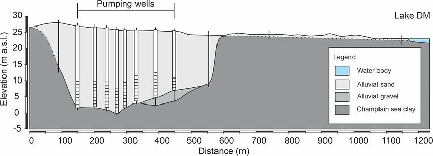
J. Masse-Dufresne et al.: Quantifying floodwater impacts on a lake water budget 3735
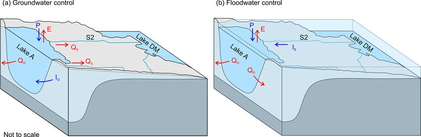
Figure 3. Schematic representation of the hydrological processes at lake A during (a) groundwater control and (b) floodwater control
periods. Inputs include precipitation (P ), surface water (IS ), and groundwater (IG ), while outputs include evaporation (E), surface water
outflow (QS ), and groundwater outflow (QG ). The area between lake DM and lake A is flooded in (b), and IS from lake DM contribute to
the water balance of lake A.
to lake DM, except from 27 February to 8 May 2017. Dur- 3 Methods
ing this period (hereafter referred to as the floodwater con-
trol period), the water level of lake DM exceeds the to- 3.1 Field measurements
pographic threshold, and lake A receives surface water in-
flow (IS ) from lake DM. Also, it is likely that the high wa- Pressure–temperature loggers (Diver® ; TD-Diver and CTD-
ter level in lake A imposed a hydraulic gradient at the lake– Diver; Van Essen Instruments B.V., Delft, the Netherlands)
aquifer interface, which allowed for QG from the lake and in- were used to measure surface water levels at lake A and
hibited IG . Then, as lake A and lake DM water levels started groundwater levels at observation well VP on a 15 min time
to decrease (from 8 May 2017), it is assumed that water ex- step. Water levels were recorded from 27 April 2017 (af-
its lake A as surface water outputs (QS ) towards lake DM or ter the ice cover melted) to 17 May 2017 at lake A and
as QG . Although lake DM’s water level again exceeded the from 29 March 2017 to 25 January 2018 (except between
topographic threshold from November 2017 to January 2018, 19 July and 6 August 2017) at observation well VP. All
the weaker correlation between the water levels suggests that the level loggers’ clocks were synchronized with the com-
the lake A water level was not controlled by lake DM. In this puter’s clock when launching automatic measurements. This
context, we conceptualized that lake A water level variations procedure was done via the Diver-Office 2018.2 software.
are mainly controlled by groundwater flows (IG and QG ). Manual measurements of the water level were regularly per-
Surface water inputs (IS ) are set to zero during this period formed to calibrate (relative to a reference datum) and vali-
(see Sect. 2.2). date the automatic water level measurements. A level logger
To summarize, for the year 2017, the lake A water budget was also used to measure on-site atmospheric pressure and
can be conceptualized with two distinct hydrological periods, perform barometric compensation on water level measure-
i.e. (a) the groundwater control period and (b) the floodwater ments. Also note that water levels in lake A were not contin-
control period (Fig. 3). While the groundwater control period uously recorded after 17 May 2017 due to a logger failure,
concerns most of the hydrological year, the floodwater con- but manual water level measurements (in September 2017,
trol period only applies from 23 February to 8 May 2017. December 2017, and January 2018) depict the general evolu-
During the groundwater control period (Fig. 3a), it is as- tion of lake A’s water level.
sumed that groundwater inflows (IG ) and precipitation (P ) Mean daily water levels at lake DM were retrieved with
constitute the total water inputs to lake A, while surface wa- permission from the Centre d’expertise hydrique du Que-
ter inflows (IS ) are negligible. During this period, the outputs bec database (Centre d’expertise hydrique du Québec, 2020).
are occurring through evaporative fluxes (E), surface water Meteorological data were measured at land-based meteo-
outflows (QS ), and groundwater outflows (QG ). In contrast, rological stations near the study site and obtained from
it is assumed that IS and P represent the total water inputs to the Environment and Climate Change Canada database
lake A during the floodwater control period (Fig. 3b). High (available online at https://www.weatherstats.ca/, last access:
water levels at lake A impose a hydraulic gradient at the lake– 30 September 2019). Daily air temperature, relative humid-
aquifer interface, which allows for QG and inhibits IG . ity, wind speed, dew point, and atmospheric pressure were
measured at the Montréal–Mirabel International Airport sta-
tion (45.68◦ N, −74.04◦ E; 18 km from the study site). Daily
precipitation and solar radiation were measured at Sainte-
Anne-de-Bellevue station (45.43◦ N, −73.93◦ E; 10 km from
https://doi.org/10.5194/hess-25-3731-2021 Hydrol. Earth Syst. Sci., 25, 3731–3757, 2021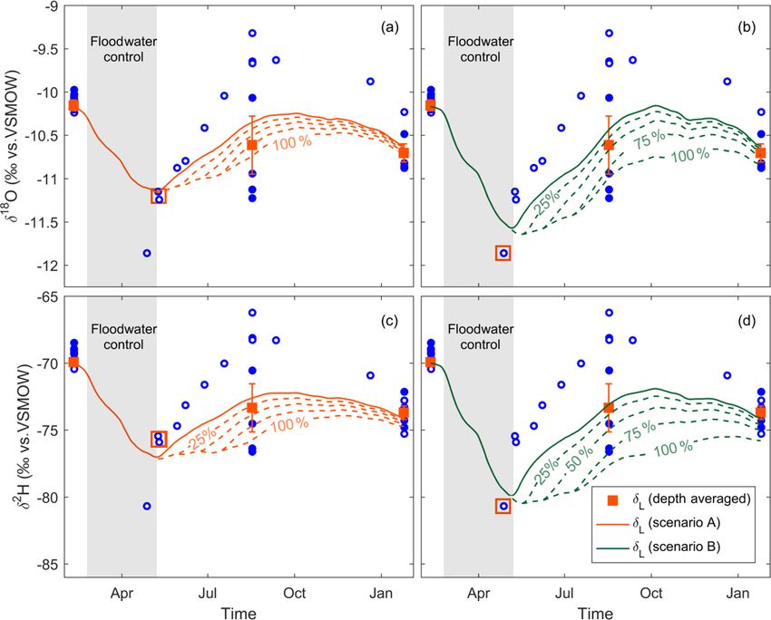
3736                                       J. Masse-Dufresne et al.: Quantifying floodwater impacts on a lake water budget

the study site) and Montréal–Trudeau International Airport          Quebec). In total, 1 mL of water was pipetted in a 2 mL
station (45.47◦ N, −73.75◦ E; 17 km from the study site), re-       vial and closed with a septum cap. Each sample was in-
spectively.                                                         jected (1 µL) and measured 10 times. The first two injec-
                                                                    tions of each sample were rejected to limit memory effects.
3.2    Water sampling and analytical techniques                     A total of three internal reference waters (δ 18 O = 0.23 ±
                                                                    0.06 ‰, −13.74 ± 0.07 ‰ and −20.35 ± 0.10 ‰; δ 2 H =
Physico-chemical parameter measurements and water sam-              1.28 ± 0.27 ‰, −98.89 ± 1.12 ‰, and −155.66 ± 0.69 ‰)
pling were performed at lake A at approximately 0.3 m be-           were used to normalize the results on the Vienna Standard
low the surface and 1 m from the lake shoreline (at LA-             Mean Ocean Water–Standard Light Antarctic Precipitation
S1) on a weekly to monthly basis from 9 February 2017               (VSMOW–SLAP) scale. A fourth reference water (δ 18 O =
to 25 January 2018. Physico-chemical parameters (including          −4.31 ± 0.08 ‰; δ 2 H = −25.19 ± 0.83 ‰) was analysed as
temperature, electrical conductivity, pH, and redox poten-          an unknown to assess the exactness of the normalization. The
tial) were measured using a multiparameter probe (YSI Pro           overall analytical uncertainty (1σ ) is better than ±0.1 ‰ for
Plus 6051030 and Pro Series pH/ORP/ISE and Conductivity             δ 18 O and ±1.0 ‰ for δ 2 H. This uncertainty is based on the
Field Cable 6051030-1; YSI Incorporated, Yellow Springs,            long-term measurement of the fourth reference water and
OH, USA). Additionally, vertical profile measurements and           does not include the homogeneity nor the representativity of
depth-resolved water sampling were conducted on 9 Febru-            the sample.
ary 2017, 17 August 2017, and 25 January 2018 (at LA-P1
to LA-P4). Lake A water sampling was performed in the               3.3   Stable isotope mass balance
northern part of the lake for logistical reasons and due to ease
of accessibility. As horizontal homogeneity has been previ-         Stable isotope mass balances for lakes can either be per-
ously demonstrated by Pazouki et al. (2016), the water sam-         formed based on (i) a well-mixed single layer model or (ii) a
ples were deemed representative of the whole waterbody.             depth resolved multi-layered model. Arnoux et al. (2017c)
   Floodwater was sampled at two locations (near S2 and S3)         performed a comparison of both methods and reported that
on 19 April 2017 and at lake DM on 10 May 2017. Water               well-mixed and depth-resolved multi-layered models yielded
samples were also collected at the surface and at depth within      similar results and showed that groundwater inputs and out-
lake B and at observation well Z16, which is upstream of            puts play an important role in lake water budgets. Arnoux
lake B and, thus, representative of the regional groundwater        et al. (2017c) further highlighted that the multi-layer model
contributing to the latter (Ageos, 2016).                           additionally allowed for the determination of groundwater
   Water samples were analysed for major ions, alkalinity,          flow with depth but required a temporally and depth-resolved
and stable isotopic compositions of water (δ 18 O and δ 2 H).       sampling in order to ensure a thorough understanding of the
Water was filtered in the field using 0.45 µm hydrophilic           stability/mixing of the different layers. Such time-consuming
polyvinylidene fluoride (PVDF) membranes (Millex-HV;                sampling and monitoring efforts are, however, often unreal-
Millipore, Burlington, MA, USA) prior to sampling for               istic in remote and/or flood-affected contexts. Additionally,
major ions and alkalinity. From December to March, cold             Gibson et al. (2017) showed that the timing of the lake water
weather prevented field filtration, so this procedure was per-      sampling may introduce greater bias in a well-mixed isotopic
formed in the laboratory on the same day. All samples were          mass balance model than the uncertainty related to the lake
collected in 50 mL polypropylene containers and cooled dur-         stratification. For these reasons, we opted to develop a well-
ing transport to the laboratory. The samples were then kept         mixed model in the context of this study. Note that, despite
refrigerated at 4 ◦ C until analysis, except for stable isotopes,   the biases underlying well-mixed models, this approach re-
which were stored at room temperature. Major ions were              mains adequate for characterizing the relative importance of
analysed within 48 h via ionic chromatography (ICS 5000             hydrological processes and is particularly useful for giving
AS-DP Dionex; Thermo Fisher Scientific, Saint-Laurent,              first-order estimates of water fluxes in ungauged basins.
QC, Canada) at Polytechnique Montréal (Montreal, Que-                  The water and stable isotope mass balance of a well-mixed
bec). The limit of detection was ≤ 0.2 mg L−1 for all ma-           lake can be described, respectively as Eqs. (1) and (2) as fol-
jor ions. Bicarbonate concentrations were derived from al-          lows:
kalinity, which was measured manually in the laboratory ac-         dV
cording to the Gran method (Gran, 1952) at Polytechnique                 = I −E−Q                                              (1)
                                                                     dt
Montréal (Montreal, Quebec). On samples with measured                 dδL       dV
alkalinity (n = 12), the ionic balance errors were all be-          V      + δL    = I δI − EδE − QδQ ,                        (2)
                                                                        dt      dt
low 8 %. The mean and median ionic balance errors were
1 %. Stable isotopes of oxygen and hydrogen were measured           where V is the lake volume, t is time, I is the instantaneous
with a water isotope analyser with off-axis integrated cavity       inflow, E is evaporation, and Q is the instantaneous out-
output spectroscopy (LGR-T-LWIA-45-EP; Los Gatos Re-                flow. I corresponds to the sum of surface water inflow (IS ),
search, San Jose, CA, USA) at Geotop-UQAM (Montreal,                groundwater inflow (IG ), and precipitation (P ). Similarly,

Hydrol. Earth Syst. Sci., 25, 3731–3757, 2021                                        https://doi.org/10.5194/hess-25-3731-2021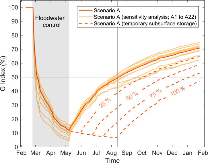
J. Masse-Dufresne et al.: Quantifying floodwater impacts on a lake water budget                                                3737

Q is the sum of surface water outflow (QS ) and groundwater           suming bank slopes of 20 or 30◦ , a typical range for sat-
outflow (QG ). δL , δI , δE , and δQ are the isotopic composi-        urated sands (Holtz and Kovacs, 1981), would result in an
tions of the lake, I , E, and Q, respectively. In the context         estimated initial lake volume of 4.84 × 10⁶ m3 (+3 %) and
of this study, the balance equations can be simplified based          4.32 × 10⁶ m3 (−8 %). Lake A volume variations are esti-
on the conceptual model. During the groundwater control pe-           mated from daily water level changes and assuming a con-
riod, IS = 0 and, thus, I = IG +P and δI = (δG IG +δP IP )/I .        stant lake area. As water level measurements are only avail-
In contrast, IG = 0 during the floodwater control period,             able for a short period at lake A, water levels at lake DM
I = IS +P and δI = (δIs IS +δP IP )/I . Note that δG and δIs are      and observation well VP are used as proxies. Water levels
the isotopic signatures of groundwater and surface water in-          at observation well VP were used as a proxy from 24 Au-
puts, respectively.                                                   gust to 30 October 2017, while water levels at lake DM were
   The application of Eqs. (1) and (2) for both δ 18 O and δ 2 H      assumed representative of lake A for the rest of the study
is valid during the ice-free period and also assumes the con-         period (i.e. from 9 February to 23 August 2017 and from
stant density of water (Gibson, 2002). In this study, the po-         31 October 2017 to 25 January 2018). This approximation is
tential impacts of the ice cover formation and melting are ne-        deemed acceptable because the simulation of δL depends on
glected, as the ice volume is likely to represent only a small        the remaining fraction of lake water f (not the absolute wa-
fraction (< 2 %) of the entire water body. Moreover, consid-          ter level), and daily variations in the water levels at lake A,
ering the ice water isotopic separation factor, i.e. 3.1 ‰ for        lake DM, and observation well VP were shown to be similar
δ 18 O and 19.3 ‰ for δ 2 H (O’Neil, 1968) and assuming well-         (see Sect. 2.2).
mixed conditions, the lake water isotopic variation would be             Evaporative fluxes (E) are calculated using the stan-
comprised within the analytical uncertainty. Also, floodwater         dardized Penman-48 evaporation equation, as described in
inputs from lake DM were expected to be much more impor-              Valiantzas (2006), as follows:
tant and occurring simultaneously with ice melt during the                            1   Rn    γ    6.43f (u)D
freshet period.                                                       EPenman-48 =      ·    +     ·            ,                (5)
                                                                                     1+γ λ     1+γ       λ
   Thus, a volume-dependent model is applied, as described
in Gibson (2002). The change in the isotopic composition of           where Rn is the net solar radiation (megajoules per square
the lake (δL ) with f (i.e. the remaining fraction of lake water)     metre per day), 1 is the slope of the saturation vapour
can be expressed as Eq. (3) as follows:                               pressure curve (kilopascals per degree Celsius; hereafter
                              h
                                  −(1+mX)
                                            i                         kPa ◦ C−1 ), γ is the psychrometric coefficient (kPa ◦ C−1 ),
δL (f ) = δS − (δS − δ0 ) f        1−X−Y
                                                ,              (3)    λ is the latent heat of vaporization (megajoules per kilo-
                                                                      gram), f (u) is the wind function (see Appendix B), and D is
where X = E/I is the fraction of lake water lost by evapora-          the vapour pressure deficit. For comparative purposes, esti-
tion, Y = Q/I is the fraction of lake water lost to liquid out-       mation of the daily evaporative fluxes was also conducted
flows, m is the temporal enrichment slope (see Appendix B),           with the Linacre-OW equation (Linacre, 1977) and the sim-
δ0 is the isotopic composition of the lake at the beginning of        plified Penman-48 equation (Valiantzas, 2006). These meth-
the time step, and δS is the steady-state isotopic composition        ods yielded similar evaporation estimates from April to Au-
the lake would attain if f tends to 0 (see Appendix B).               gust but underestimated total evaporation by 24 % to 33 %
   A step-wise approach is used to solve Eq. (3) on a daily           compared to the standardized Penman-48 equation. The dis-
time step. At each time step, recalculation of f = V /V0 is           crepancy between the models is restricted to late summer and
needed, where V is the residual volume at the end of the              autumn (see Appendix C; Fig. C1) and is attributed to the dif-
time step and V0 the original volume at the beginning of the          ference between the air and water surface temperature, which
time step (or V t−dt ). Hence, Eq. (3) is based on the water          was estimated based on the equilibrium method as described
level difference between 2 d. The water flux parameters (E,           by de Bruin (1982; see Appendix D). Note that E and P are
I, and Q) and isotopic signatures (δE , δA , δI , and δQ ) are thus   set to zero during the ice cover period (i.e. from 1 January to
evaluated on a daily time step.                                       31 March, based on meteorological data and field observa-
   The flushing time (tf ) is defined as the ratio of the volume      tions).
of water in a system to the rate of renewal (Monsen et al.,              For well-mixed conditions, the δQs and δQg are assumed
2002). In this study, tf by groundwater inputs is considered          to be equal to δL . Hence, no separation of these two fluxes
and is expressed as follows:                                          is attempted, and they are merged into one variable, i.e. the
                                                                      outflow (Q). The direction and intensity of the water flux
tf = V /IG .                                                   (4)
                                                                      at the lake–aquifer interface can be conceptually described
3.4   Daily volume changes at lake A and water fluxes                 by Darcy’s law, which states that Q = KAi, where K is the
                                                                      hydraulic conductivity, A is the cross-sectional area through
The initial lake volume (4.7 × 10⁶ m3 ) was estimated from            which the water flows, and i is the hydraulic gradient. Given
the observed lake surface area (2.79 × 10⁵ m2 ) and the max-          the significant depth of lake A (i.e. 20 m) in comparison to
imal depth (20 m) and assuming bank slopes of 25◦ . As-               the maximum water level change during the flooding event

https://doi.org/10.5194/hess-25-3731-2021                                          Hydrol. Earth Syst. Sci., 25, 3731–3757, 2021
3738 J. Masse-Dufresne et al.: Quantifying floodwater impacts on a lake water budget
(i.e. 2.7 m), the variations in A and K are expected to have
a minor impact on Q. Hence, the change in outflows from
the lake is expected to be mainly controlled by i changes
and, consequently, to be roughly proportional to the change
in lake water level. Considering the above, it was assumed
that the daily outflow flux from lake A varied linearly ac-
cording to the lake water level; the minimum and maximum
outflow (Qmin and Qmax ) correspond to the minimum and
maximum water level, respectively. The outflow range (i.e.
minimum and maximum values) was adjusted to obtain the
best fit between the calculated and observed δL .
Total daily inflow (sum of daily P , IS , and IG ) into lake A
compensates for the adjusted daily outflow and daily lake
volume difference. The precipitation (P ) is evaluated from
the available meteorological data (see Sect. 3.1), while direct
measurement of IS and IG was not possible in this hydro-
geological context (see Sect. 2.1). Consequently, further as-
sumptions are needed to apportion these contributions. Con-
sidering the proposed conceptual model of the groundwater–
surface water interactions (see Sect. 2.2), IS is set to zero,
while IG is contributing to the lake during the groundwa-
ter control period. On the other hand, during the floodwater
control period (i.e. from 23 February to 8 May 2017), it is
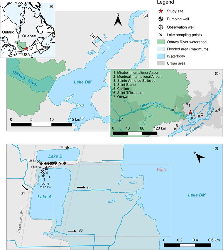
Figure 4. Isotopic composition of precipitation, lake A water, and
assumed that the rising water level at lake A results in a hy- floodwater from March 2017 to January 2018. Hollow and solid
draulic gradient forcing the lake water to infiltrate into the blue circles correspond to samples collected at ≤ 2 and > 2 m depth,
aquifer, inhibiting IG . respectively. Analytical precision is 0.15 ‰ and 1 ‰ at 1σ for δ 18 O
and δ 2 H. Precipitation data are retrieved from the research infras-
tructure on groundwater recharge database (Barbecot et al., 2019).
4 Results
outputs, the inflows to lake A must therefore be greater than
From 23 February to 8 May 2017, the net water fluxes are the net water fluxes.
mainly positive, and an overall volume increase is observed For that reason, the development of a volume-dependent
at lake A. The maximum volume change of lake A was transient stable isotope mass balance was required to cor-
7.6 × 10⁵ m3 , which represents 16 % of the lake’s initial vol- rectly depict the importance of the floodwater inputs on the
ume. The maximum net water flux was 1.2×10⁵ m3 d−1 , cor- water mass balance of the lake.
responding to a water level rise of 0.43 m (on 5 April 2017
only). From 9 May to mid-August 2017, lake A volume was 4.1 Isotopic and geochemical framework
decreasing, and the daily net water fluxes were mainly neg-
ative. In early August 2017, lake A regained its initial vol- The isotopic composition of precipitation (δP ), lake A, and
ume. Then, in autumn and winter, the volume of lake A floodwater are depicted in Fig. 4. The local meteoric water
was oscillating, and the net water fluxes were ranging from line (LMWL) was defined using an ordinary least squares re-
−6.4 × 10⁴ to 5.3 × 10⁴ m3 d−1 . At the end of the study gression (Hughes and Crawford, 2012) using isotope data in
period (i.e. on 25 January 2018), a net volume difference precipitation from the Saint-Bruno station RIGR (Research
of 1.5 × 10⁵ m3 remained at lake A compared to 9 Febru- Infrastructure on Groundwater Recharge) database (n = 27;
ary 2017. from December 2015 to June 2017).
However, the evolution of lake A volume and the net For the study period, the isotopic composition of bulk pre-
water fluxes are not representative of the surface water– cipitation was available on a biweekly to monthly time step
groundwater interactions. Indeed, gross water fluxes are (n = 15) and ranged from −19.19 ‰ to −6.85 ‰ for δ 18 O
likely to exceed net water fluxes at natural and dredged and −144 ‰ to −38 ‰ for δ 2 H. Interpolation was used to
lakes sitting in permeable sediments (Zimmermann, 1979; simulate the δP on a daily time step for the isotope mass bal-
Arnoux et al., 2017a; Jones et al., 2016). In the context of ance model computation.
this study, we conceptualized two main hydrological periods Isotopic compositions of lake A water samples (n = 39)
during which the lake water can either drain towards lake DM are linearly correlated (see solid blue line) and all plotted
or exit the lake as groundwater output. To balance out these below the LMWL, which confirms that lake A is influenced
Hydrol. Earth Syst. Sci., 25, 3731–3757, 2021 https://doi.org/10.5194/hess-25-3731-2021J. Masse-Dufresne et al.: Quantifying floodwater impacts on a lake water budget 3739
by evaporation. Linear regression of lake A water samples
defines the local evaporation line (LEL), which is δ 2 H =
5.68(±0.27) · δ 18 O − 12.80(±2.83) (R 2 = 0.92). Some sam-
ples from the surface of lake A are plotted below the LEL,
likely indicating snowmelt water inputs as noted in previous
studies of Canadian lakes (Wolfe et al., 2007).
The isotopic composition of the floodwater samples (n =
3) is indeed more depleted than lake A waters (i.e. δ 18 O from
−11.85 ‰ to −11.18 ‰ and δ 2 H from −81 ‰ to −78 ‰)
and is most likely reflecting the significant contribution from
heavy isotope-depleted snowmelt waters. The floodwater
samples are also linearly correlated and are plotted along a
line (δ 2 H = 5.33δ 18 O − 18.82) for which the slope is similar
to lake A LEL, suggesting that the sampled floodwater evap-
orated under the same conditions as lake A water samples.
For simplification purposes, the isotopic composition of the
surface water inflow (δIs ) was set to the intersection between
the floodwater LEL and the LMWL (δ 18 O = −12.00 ‰ and
δ 2 H = −83 ‰). The long-term (1997–2008) average and
minimum and maximum isotopic signatures of Ottawa River Figure 5. Geochemical facies of lake A (n = 23) and floodwater
water at Carillon (∼ 34 km upstream from lake DM; see (n = 1). Mean values for lake B (n = 42) and regional groundwa-
Fig. 1b) for the month of April are −11.19 ‰, −12.01 ‰ and ter (GW) (n = 11) geochemical facies are also plotted. Lake A and
floodwater are characterized by Ca-HCO3 water types, while lake B
−10.23 ‰ for δ 18 O and −81 ‰, −85 ‰ and −77 ‰ for δ 2 H,
and regional GW correspond to Na-Cl water types. Note that re-
respectively (Rosa et al., 2016). The mean and minimum val- gional GW was sampled upstream of lake B.
ues compare well with the observed isotopic signatures at
lake DM during springtime in 2017.
The isotopic composition of groundwater (δG ) can be de- and reveals a depth-wise homogeneity. The geochemistry of
termined from direct groundwater samples or indirectly from lake B is distinct from lake A and appears to be influenced by
the amount-weighted mean δP . However, in highly seasonal regional groundwater characterized by a Na-Cl water type.
climates, there is a widespread cold season bias to ground-
water recharge (Jasechko et al., 2017), and estimating δG via 4.2 Evaluation of the water budget
groundwater samples or an amount-weighted mean δP may
be misleading. In fact, it has been argued that the LMWL– 4.2.1 Volume dependent isotopic mass balance model
LEL intersection better represents the isotopic composition
of the inflowing water to a lake and is, thus, commonly used As described in Sect. 3.3, the isotopic mass balance model
to depict the δG in isotopic mass balance applications (Gib- was solved iteratively by recalculating δL on a daily time
son et al., 1993; Wolfe et al., 2007; Edwards et al., 2004). step. This model was developed assuming (1) well-mixed
Concerning the study site, the estimated δG is −11.26 ‰ for conditions and (2) that the outflow flux changes are roughly
δ 18 O and −77 ‰ for δ 2 H (i.e. the Saint-Bruno LMWL and proportional to the lake’s water level changes. We adjusted
lake A LEL intersection). The latter compares well with the the minimum and maximum outflow fluxes (Qmin and Qmax )
mean isotopic signature of groundwater at Saint-Télesphore so that they corresponded to the minimum and maximum wa-
station (−11.1 ‰ for δ 18 O and −78.5 ‰ for δ 2 H; Barbe- ter levels (see Fig. 3).
cot et al., 2018) and is more depleted than the long-term In total, three sampling campaigns (i.e. on 9 Febru-
amount-weighted mean δP at Ottawa (−10.9 ‰ for δ 18 O and ary 2017, 17 August 2017, and 25 January 2018) were con-
−75 ‰ for δ 2 H; IAEA/WMO, 2018). Note that the loca- ducted at lake A in order to collect water samples for iso-
tions of Saint-Télesphore station and Ottawa are depicted in topic analyses from the epilimnion, metalimnion, and hy-
Fig. 1b. polimnion (Fig. 6; Appendix E; Fig. E1) to account for the
The geochemical facies of lake A and lake DM sam- vertical stratification of the isotopic signature (Gibson et al.,
ples are illustrated in Fig. 5 by the means of a Piper di- 2017). The vertical isotopic profiles were volume-weighted
agram. Mean values for lake B and regional groundwa- according to the representative layer for each discrete mea-
ter (GW) geochemical facies are also plotted for compar- surement in order to obtain the observed δL for each cam-
ison purposes. Both lake A and floodwater were found to paign (Table 1). The depth-averaged isotopic composition
be Ca-HCO3 types, which is typical for precipitation- and of the lake on 9 February 2017 (i.e. δ 18 O = −10.15 ‰ and
snowmelt-dominated waters (Clark, 2015). The geochem- δ 2 H = −70 ‰) was used as the initial modelled δL .
istry of lake A is relatively constant throughout the year
https://doi.org/10.5194/hess-25-3731-2021 Hydrol. Earth Syst. Sci., 25, 3731–3757, 20213740 J. Masse-Dufresne et al.: Quantifying floodwater impacts on a lake water budget
Figure 6. Observed and modelled depth-average isotopic composition of the lake (δL ) for δ 18 O (a, b) and δ 2 H (c, d) from 9 February 2017
to 25 January 2018 for scenarios A and B. The hollow and solid blue circles correspond to lake A water samples collected at ≤ 2 and
> 2 m, respectively. The modelled δL is fitted against the three depth-averaged δL and an additional sample collected at ≤ 2 m depth on
9–10 May 2017 (scenario A) and 27 April 2017 (scenario B). These samples are marked by the hollow red squares. The grey shaded area
corresponds to the floodwater control period. The error bars correspond to the standard error in the samples for each campaign. The dashed
lines represent the modelled δL when considering that 25 % to 100 % of the outputs from the lake during the floodwater control period were
temporally stored in the aquifer and discharged to the lake as floodwater-like inputs (δIs ).
Table 1. Observed depth averaged (or mean) and standard deviation (SD) of isotopic composition of lake A for the sampling campaigns in
February 2017, August 2017, and January 2018 and all samples. The isotopic composition of the samples collected at the surface of lake A
on 9–10 May and 27 April 2017 are also listed. The asterisks (∗ ) indicate that a mean value was calculated (instead of a depth-averaged
value).
Period Date n δ 18 O (‰) δ 2 H (‰)
Depth SD Depth SD
averaged averaged
Groundwater control 9 Feb 2017 9 −10.15 0.11 −69.92 0.41
9–10 May 2017 (scenario A) 2 −11.20 0.05 −75.68 0.23
Floodwater control
27 April 2017 (scenario B) 1 −11.86 – −80.68 –
Groundwater control 17 Aug 2017 7 −10.61 0.82 −73.33 4.41
Groundwater control 25 Jan 2018 6 −10.70 0.26 −73.70 1.22
All samples 34 −10.32∗ 0.62 −71.35∗ 3.69
While depth-averaged δL was not available during the riod, and that the water samples collected at the surface of
floodwater control period (i.e. late February to early May), lake A on 27 April or 9–10 May 2017 are representative
water samples from the surface of lake A provide rele- of the whole water body. Indeed, the observed surface wa-
vant evidence to better constrain the model. It is likely that ter temperature was < 5 ◦ C until early May (see Fig. C1)
lake A was fully mixed during the floodwater control pe- and suggests a limited density gradient along the water col-
Hydrol. Earth Syst. Sci., 25, 3731–3757, 2021 https://doi.org/10.5194/hess-25-3731-2021J. Masse-Dufresne et al.: Quantifying floodwater impacts on a lake water budget 3741
umn which does not allow for the development of ther- ios, despite the intensity of the flood event. For scenarios A
mal stratification. In this context, we opted to simulate two and B, tf , as defined in Eq. (4), is similar (i.e. 135 and 110 d).
scenarios (A and B) for which the isotopic mass balance Precipitation is contributing 1 % of the total annual inputs
model is either constrained at δ 18 O = −11.20 ‰ andδ 2 H = and evaporation only accounts for 2 % of the total annual
−76 ‰ on 9–10 May 2017 or at δ 18 O = −11.86 ‰ and outputs. Although the establishment of a hydraulic connec-
δ 2 H = −80.68 ‰ on 27 April 2017. tion between lake DM and lake A is a recurring yearly hy-
The results of the volume-dependent isotopic mass bal- drological process, it is important to note that the magnitude
ance for δ 18 O and δ 2 H are illustrated in Fig. 6. The fit- and duration of the flooding event of 2017 was particularly
ted Qmin and Qmax from lake A are 3.7 × 10⁴ and 8.0 × important and, thus, had a greater impact on the dynamic of
104 m3 d−1 for scenario A and 1.0×10³ and 2.8×10⁵ m3 d−1 lake A in comparison to other years.
for scenario B. These first-order water flux estimates repre-
sent equivalent water level variations ranging from 0.004 and 4.2.2 Sensitivity analysis
1.0 m d−1 . From 23 February to 8 May 2017 (see the grey
shaded area), hydraulic conditions allowed for surface in- A one-at-a-time (OAT) sensitivity analysis was performed to
puts (IS ) from lake DM to lake A at a mean rate of 6.61 × grasp the relative impact of the input parameters’ uncertain-
104 m3 d−1 , with a total floodwater volume of 4.82 × 10⁶ m3 ties on the model outputs. For each parameter, we tested two
for scenario A. The total floodwater volume was twice scenarios which delimit the uncertainty for each parameter.
as important (9.96 × 10⁶ m3 ) for scenario B. Then, from First, we tested the sensitivity of the model for V + 3 % and
9 May 2017, we considered that these floodwater inputs V − 8 % (i.e. estimated with slopes of 30 and 20◦ ). Con-
stopped as the lake water level started to decrease. As a con- cerning δIs and δG , the model was tested for ±0.5 ‰ for
sequence, the model yielded a gradual enrichment of δL due δ 18 O and ±4 ‰ for δ 2 H, assuming they would both evolve
to the combined contribution from IG and E for both sce- along the LMWL (see Fig. 3). Then, we assessed the sen-
narios. From 9 May 2017 to 25 January 2018, the total IG sitivity of the model to δA by fixing the seasonality fac-
were 1.16 × 10⁷ and 1.48 × 10⁷ m3 for scenario A and B, re- tor k at 0.5 and 0.9. Evaporation was computed with ±20 %,
spectively. Overall, the δ 18 O and δ 2 H models were better at whereas the meteorological parameters (i.e. relative humid-
reproducing the January 2018 and August 2017 observed δL , ity (RH), Tair , U , P , and Rs) were tested for ±10 %. As
respectively. This is likely linked to the uncertainties and rep- E and δA are dependent on the water surface temperature,
resentativeness of the meteorological data, which is control- we also tested the sensitivity of the model when consider-
ling the isotopic fractionation due to evaporation. ing that T is equal to the daily mean air temperature (Tair ).
While the computed flows for scenario A are within a plau- Finally, we tested for the uncertainties concerning the defi-
sible range for the combination of surface and groundwater nition of the LMWL. For the reference scenario, the LMWL
outflow processes (i.e. minimum and maximum equivalent (δ 2 H = 8.13 · δ 18 O + 14.78) was estimated using an ordinary
water level variations of 0.13 and 0.29 m d−1 ), scenario B least square regression (OLSR). For the sensitivity analysis,
yielded less realistic results (i.e. minimum and maximum we estimated the LMWL via a precipitation amount weighted
equivalent water level variations of 0.004 and 1.0 m d−1 ). least square regression (PWLSR), which was developed by
As mentioned above, scenario B was constrained at δ 18 O = Hughes and Crawford (2012). Using the PWLSR method, the
−11.86 ‰ and δ 2 H = −80.68 ‰ in late April (Fig. 6), based LMWL is defined as δ 2 H = 8.28 · δ 18 O + 17.73, and δIs and
on a surface water sample which was taken during a tem- δG are estimated at −12.39 ‰ and −11.74 ‰ for δ 18 O and
porarily decreasing water level period (Fig. 3) and is, thus, at −85 ‰ and −79 ‰ for δ 2 H, respectively. Recalculation
likely less representative of the overall lake’s dynamics com- of δIs and δG was needed, as they were both assumed to be
pared to scenario A. This demonstrates the limit of the ap- plotted on the LMWL (see Sect. 4.1).
proach and shows that it is important to correctly constrain The results of this sensitivity analysis are listed in Ta-
the model during flood events in order to perform precise es- bles F1 and F2 (Appendix F) for scenarios A and B. Overall,
timations of the water balance. the model was found to be highly sensitive to the uncertain-
The water mass balance of lake A from 9 February 2017 ties associated with δIs , δG , and E, as the annual mean water
to 23 January 2018 is summarized in Table 2 for both scenar- fluxes (Q and I ) varied up to −31 % and +46 % compared
ios. The difference between the total inputs and total outputs to the reference scenarios A and B. A negligible to slight
correspond to the lake volume difference (1.48×10⁵ m3 ) be- change in the modelled δL was found when considering the
tween the start and the end of the model run. Groundwater uncertainties for V , δA , RH, Tair , U , P , and Rs. For these
inputs (IG ) and surface water inputs (IS ) account for 71 % variables, the mean flux estimate (Q and I ) changes ranged
and 28 % of the total water inputs to the lake for scenario A. from −8 % to +4 % compared to the reference scenarios A
While IS are twice as important for scenario B, they only ac- and B. As expected, the value of δIs affects the modelled δL
count for 39 % (+11 %) of the total inputs, and the IG are exclusively during the floodwater control period. Similarly,
60 % (−11 %). It thus appears that the annual dynamic of the values of δG and E particularly influence the modelled δL
lake A is dominated by groundwater inputs for both scenar- from late summer to early winter. This is due to the fact that
https://doi.org/10.5194/hess-25-3731-2021 Hydrol. Earth Syst. Sci., 25, 3731–3757, 20213742 J. Masse-Dufresne et al.: Quantifying floodwater impacts on a lake water budget
Table 2. Water mass balance of lake A for scenarios A and B. The difference between the total inputs and total outputs corresponds to the
lake volume difference over the study period. The total inputs (I ) correspond to the sum of precipitation (P ), surface water inflow (IS ), and
groundwater inflow (IG ). The total outputs (Q) correspond to the sum of evaporation (E) and surface water and groundwater outflow (Q).
The mean flushing time (tf ) is the ratio of the lake volume to the mean groundwater inputs (IG ).
Scenario Inputs (×106 m3 ) Total I Outputs (×106 m3 ) Total Q tf
P IS IG (×106 m3 ) E Q (×106 m3 ) (Days)
A 0.2 4.8 12.2 17.3 0.4 16.8 17.2 135
B 0.2 10.0 15.1 25.3 0.4 24.8 25.2 110
0.0 5.1 2.9 8.0 0.0 8.0 8.0 −25
Difference
0% +107 % +24 % +46 % 0% +48 % +47 % −19 %
Q and E are the dominant fluxes during this period. When the importance of floodwater inputs in the water balance par-
considering that T is equal to Tair , despite the significantly tition.
different maximum and minimum values for Q, the mean Q Assuming that 25 % to 100 % of the outputs (Q) from the
was relatively similar to the reference scenarios, and only a lake during the floodwater control period were temporally
small change for tf (+3 % and +2 % compared to reference stored in the aquifer and did eventually discharge back to
scenarios A and B) was found. Finally, the model is highly the lake, the modelled δL diverges more or less from the ref-
sensitive to the uncertainties associated with the LMWL, as a erence scenarios A and B (Fig. 6; see the dashed lines). It
translation of the LMWL implies an enrichment or depletion is noteworthy that a better fit between the modelled δL and
of both the δIs , δG at the same time. Such modifications result depth-averaged δL is obtained when considering that 25 %
in mean flux estimate (Q and I ) changes of up to −38 % and to 50 % of the outputs (Q) from the lake during the flood-
−43 % compared to reference scenarios A and B. water control period discharge back to the lake. In fact, it is
likely that part of the potential stored floodwater could have
4.3 Importance of temporary floodwater storage on the effectively discharged back to the lake. For instance, part of
water balance partition the floodwater-like groundwater could have been abstracted
by the pumping wells at the adjacent bank filtration site or
The developed isotopic mass balance model yielded signif- could have been discharged to lake B. These results illustrate
icant floodwater inputs during springtime to be a best fit to the importance of considering temporary subsurface flood-
the observed δL . A first-order estimate of the total floodwater water storage when assessing water balances, especially as
volume summed to 4.82 × 10⁶ m3 (for scenario A), which is the magnitude and frequency of floods are likely to be more
nearly equal to the lake’s initial volume (i.e. 4.70 × 10⁶ m3 ). important in the future (Aissia et al., 2012).
Similar results were obtained by Falcone (2007), who stud-
ied the hydrological processes influencing the water balance 4.4 Temporal variability in the water balance partition
of lakes in the Peace–Athabasca Delta, Alberta (Canada) us-
ing water isotope tracers. They reported that a springtime The water balance presented in Table 2 provides an overview
freshet (in 2003) did replenish the flooded lakes from 68 % of the relative importance of the hydrological processes at
to > 100 % (88 % on average). lake A for the study period (i.e. February 2017 to Jan-
As mentioned in Sect. 2.3, it was conceptualized that the uary 2018). As the surface water inputs (as floodwater) only
high surface water elevation of lake A during springtime re- occurred during springtime at lake A, it is also important to
sulted in hydraulic gradients that forced lake water to infil- decipher the temporal variability in the water fluxes. The de-
trate into the aquifer and induce local recharge (see Fig. 3). pendence of a lake on groundwater can be quantified via the
An important volume of flood-derived water could, thus, be G index, which is the ratio of cumulative groundwater in-
stored during the increasing water level period and eventu- puts to the cumulative total inputs (Isokangas et al., 2015).
ally discharged back to the lake as its water level decreased. Figure 7 shows the temporal evolution of the G index from
Hence, the groundwater inputs to lake A following the flood- 9 February 2017 to 25 January 2018 for scenario A and the
ing event likely corresponded to flood-derived surface water associated scenarios (A1 to A22) considered in the sensitiv-
originating from lake DM. Considering that these fluxes are ity analysis. Note that the G index is calculated at a daily
characterized by a floodwater-like isotopic signature (δIs ), time step, based on the cumulative water fluxes. It is used
rather than the isotopic signature of groundwater (δG ), the to understand the relative importance of groundwater inputs
temporal evolution of the modelled δL would be modified. over the studied period and does not consider the initial state
Such a consideration is noteworthy for a better depiction of of the lake. In early February, the G index was 100 % be-
Hydrol. Earth Syst. Sci., 25, 3731–3757, 2021 https://doi.org/10.5194/hess-25-3731-2021You can also read