Integrated land and water-borne geophysical surveys shed light on the sudden drying of large karst lakes in southern Mexico
←
→
Page content transcription
If your browser does not render page correctly, please read the page content below
Solid Earth, 12, 439–461, 2021
https://doi.org/10.5194/se-12-439-2021
© Author(s) 2021. This work is distributed under
the Creative Commons Attribution 4.0 License.

Integrated land and water-borne geophysical surveys shed light on
the sudden drying of large karst lakes in southern Mexico
Matthias Bücker1,2 , Adrián Flores Orozco2 , Jakob Gallistl2 , Matthias Steiner2 , Lukas Aigner2 ,
Johannes Hoppenbrock1 , Ruth Glebe1 , Wendy Morales Barrera3 , Carlos Pita de la Paz4 , César Emilio García García4 ,
José Alberto Razo Pérez4 , Johannes Buckel1 , Andreas Hördt1 , Antje Schwalb5 , and Liseth Pérez3,5
1 Institute of Geophysics and Extraterrestrial Physics, TU Braunschweig, 38106 Braunschweig, Germany
2 Department   of Geodesy and Geoinformation, Research Unit Geophysics, TU Wien, 1040 Vienna, Austria
3 Instituto de Geología, Universidad Nacional Autónoma de México, Mexico City, 04510, Mexico
4 Geotem Ingeniería S.A. de C.V., Mexico City, 14640, Mexico
5 Institute of Geosystems and Bioindication, TU Braunschweig, 38106 Braunschweig, Germany

Correspondence: Matthias Bücker (m.buecker@tu-braunschweig.de)

Received: 6 May 2020 – Discussion started: 27 May 2020
Revised: 30 November 2020 – Accepted: 7 January 2021 – Published: 24 February 2021

Abstract. Karst water resources play an important role in        undisturbed sediment sequences on the bottom of both lakes,
drinking water supply but are highly vulnerable to even slight   which are suitable for future paleoenvironmental drilling
changes in climate. Thus, solid and spatially dense geological   campaigns, (2) develop a comprehensive geological model
information is needed to model the response of karst hydro-      implying a strong interconnectivity between surface water
logical systems to such changes. Additionally, environmental     and karst aquifer, and (3) evaluate the potential of the ap-
information archived in lake sediments can be used to un-        plied geophysical approach for the reconnaissance of the ge-
derstand past climate effects on karst water systems. In the     ological situation of karst lakes. This methodological eval-
present study, we carry out a multi-methodological geophys-      uation reveals that under the given circumstances, (i) SBP
ical survey to investigate the geological situation and sed-     and TDIP phase images consistently resolve the thickness of
imentary infill of two karst lakes (Metzabok and Tzibaná)        the fine-grained lacustrine sediments covering the lake floor,
of the Lacandon Forest in Chiapas, southern Mexico. Both         (ii) TEM and TDIP resistivity images consistently detect the
lakes present large seasonal lake-level fluctuations and ex-     upper limit of the limestone bedrock and the geometry of
perienced an unusually sudden and strong lake-level decline      fluvial deposits of a river delta, and (iii) TDIP and SRT im-
in the first half of 2019, leaving Lake Metzabok (maximum        ages suggest the existence of a layer that separates the la-
depth ∼ 25 m) completely dry and Lake Tzibaná (depth ∼           custrine sediments from the limestone bedrock and consists
70 m) with a water level decreased by approx. 15 m. Before       of collapse debris mixed with lacustrine sediments. Our re-
this event, during a lake-level high stand in March 2018, we     sults show that the combination of seismic methods, which
collected water-borne seismic data with a sub-bottom pro-        are most widely used for lake-bottom reconnaissance, with
filer (SBP) and transient electromagnetic (TEM) data with a      resistivity-based methods such as TEM and TDIP can sig-
newly developed floating single-loop configuration. In Octo-     nificantly improve the interpretation by resolving geological
ber 2019, after the sudden drainage event, we took advantage     units or bedrock heterogeneities, which are not visible from
of this unique situation and carried out complementary mea-      seismic data. Only the use of complementary methods pro-
surements directly on the exposed lake floor of Lakes Met-       vides sufficient information to develop comprehensive geo-
zabok and Tzibaná. During this second campaign, we col-          logical models of such complex karst environments
lected time-domain induced polarization (TDIP) and seismic
refraction tomography (SRT) data. By integrating the multi-
methodological data set, we (1) identify 5–6 m thick, likely

Published by Copernicus Publications on behalf of the European Geosciences Union.
440                                 M. Bücker et al.: Integrated land and water-borne geophysical surveys on karst lakes

1   Introduction                                                     Recent studies using direct-current (DC) electrical resis-
                                                                  tivity for water-borne investigations on freshwater bodies
                                                                  include surveys with floating (e.g., Befus et al., 2012; Or-
About 7 %–12 % of the world’s continental area is covered         lando, 2013; Colombero et al., 2014) or underwater elec-
by karst (e.g., Hartmann et al., 2014) and up to one-quarter      trode chains (e.g., Toran et al., 2015) and provide evidence
of the earth’s population at least partially depends on drink-    for the potential of this method for shallow-water applica-
ing water from karst systems (e.g., Ford and Williams, 2007).     tions. Electrical resistivity can also be assessed by electro-
Even though continued population growth and industrializa-        magnetic methods, which, compared to DC resistivity mea-
tion put pressure on these important resources in terms of        surements, offer a more compact experimental layout. Elec-
both water quantity and quality, the response of karst systems    tromagnetic surveys are often carried out as transient electro-
to expected future climate change is still not well understood    magnetic (TEM) soundings with floating magnetic sources
(Hartmann et al., 2014). Groundwater models offer one op-         and receivers. Hatch et al. (2010), for example, used an in-
portunity to estimate future changes in water availability but    loop configuration with a ∼ 7.5 m × 7.5 m transmitter and a
heavily depend on reliable and spatially dense geological in-     ∼ 2.5 m × 2.5 m receiver to map river bed salinization in an
formation. Where direct geological information, e.g., from        Australian river with an average water depth of 5–10 m. Mol-
drillings, is not dense enough or not available at all, geo-      lidor et al. (2013) used a similar but slightly larger setup
physical methods can be used to provide quasi-continuous          (∼ 18 m × 18 m transmitter, ∼ 6 m × 6 m receiver) to map
indirect information on the subsurface geology in karst areas     a thick conductive sediment layer below the bottom of a
(Bechtel et al., 2007).                                           20 m deep maar lake in Germany. More recently, Yogeshwar
   Another possibility to understand climatic effects on karst    et al. (2020) used the system developed by Mollidor et al. to
water systems relies on the analysis of paleoenvironmental        image a volcanic lake hydrothermal system on the Azores,
records (e.g., Medina-Elizalde and Rohling, 2012; Vázquez-        whereas Lane et al. (2020) introduced a compact floating
Molina et al., 2016). In particular, lake sediments are impor-    TEM system, designed for the rapid electrical mapping of the
tant archives of freshwater and terrestrial environmental in-     subsurface of rivers and estuaries. Some older relevant case
formation, and sediment cores can be used to reconstruct past     studies with shallow-water applications of both techniques,
climate and ecological changes in the lakes (Cohen, 2003;         DC resistivity and electromagnetic soundings, were reviewed
Schindler, 2009; Pérez et al., 2020). Thus, paleoenvironmen-      by Butler (2009).
tal studies give insight into the local links between climate        In a previous study, we successfully used geoelectrical
variations and the availability (and quality) of water in lakes   and electromagnetic methods to investigate the sedimentary
and the connected karst aquifer system. To identify suitable      infill of two desiccated lakes in a volcanic area (Bücker
drilling locations providing continuous paleoenvironmental        et al., 2017; Lozano-García et al., 2017). To extend our in-
records at a high temporal resolution, knowledge about sedi-      vestigations, in this study, we evaluate the potential of land
ment thickness and composition, depth to bedrock, and possi-      and water-borne resistivity-imaging methods to complement
ble heterogeneities within the lake sediments is needed (Last     seismic methods for the investigation of karst lakes in the
and Smol, 2002).                                                  Lacandon Forest, southern Mexico. Recent biological and
   Geophysical methods can efficiently provide such in-           abiotic studies have highlighted the great potential of sedi-
formation from the local scale up to the lake-basin scale         mentary sequences from the lakes of this remote area as con-
and can (principally) be employed on both land and wa-            tinuous paleoenvironmental and paleoclimatic records dur-
ter. Due to the usually sharp contrast between seismic ve-        ing the late Quaternary (e.g., Díaz et al., 2017; Echeverría-
locities of sediment layers and the underlying bedrock,           Galindo et al., 2019; Charqueño-Celis et al., 2020). In this
(reflection-)seismic methods are often given priority over        study, we focus on Lakes Metzabok and Tzibaná, two of the
other geophysical methods for lake-bottom reconnaissance          largest lakes of the Lacandon Forest, which experienced a
(Scholz, 2002). In particular, low-frequency echo sounders        sudden and catastrophic lake-level drop in the first half of
(e.g., Dondurur, 2018), also referred to as sub-bottom profil-    2019. While large seasonal lake-level variations are part of
ers (SBPs), allow sediment deposits of several tens of me-        the nature of both lakes, it remains unclear whether such par-
ters to be quickly mapped based on single-channel seismic         ticular events as the one observed in 2019, which left Lake
data. Nevertheless, electrical-resistivity images provided by     Metzabok completely dry, are also recurrent with a frequency
electrical resistivity tomography (e.g., Binley and Kemna,        of several decades or rather linked to recent climate change.
2005) or electromagnetic soundings (e.g., Kaufman et al.,         To better understand possible draining mechanisms and their
2014) complement the mostly geometrical information ob-           triggers, besides further paleoenvironmental investigations,
tained from reflection-seismic or sub-bottom profiling mea-       a comprehensive geological picture of the lakes’ geological
surements (Butler, 2009). Under certain conditions such as        situation is essential.
high lake-bed reflectivity and/or low reflectivity of targeted       In 2018, roughly one year before the drainage event and
boundaries, seismic methods may, however, provide insuffi-        when the lakes were filled, we collected seismic data with a
cient results, and therefore alternative methods are needed.      SBP and carried out TEM soundings to assess the electrical

Solid Earth, 12, 439–461, 2021                                                        https://doi.org/10.5194/se-12-439-2021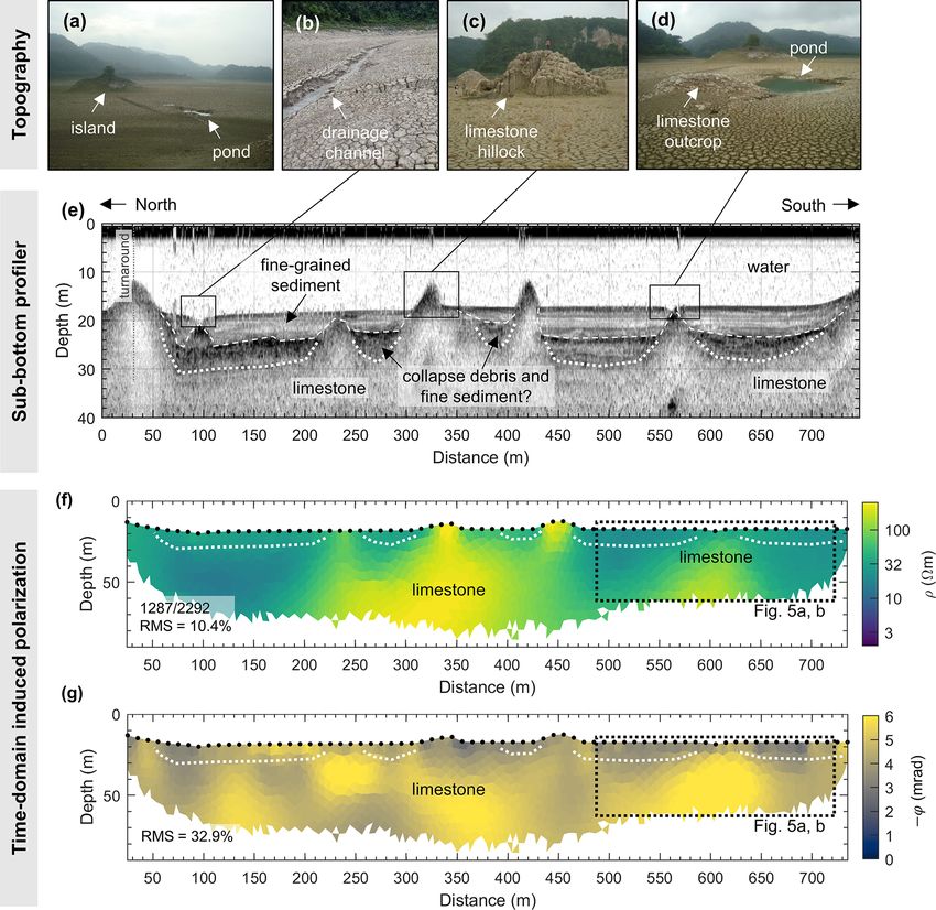
M. Bücker et al.: Integrated land and water-borne geophysical surveys on karst lakes                                             441

resistivity of the lake bottom and obtain information on the
thickness of the sedimentary infill. The sudden drainage of
the investigated lakes in 2019 provided us with the unique
opportunity to collect additional data directly on the dry lake
bed. Seismic data were then recollected with a seismic refrac-
tion tomographic (SRT) setup in order to provide information
on both refractor geometry and seismic velocities of the dif-
ferent geophysical units. Additional electrical imaging data
were measured with the time-domain induced polarization
(TDIP) method, which has fewer limitations regarding the
detectability of thin near-surface layers and heterogeneities
than the transient electromagnetic method. Furthermore, the
polarization properties of the subsurface materials assessed
by TDIP measurements provide additional information and
can improve the interpretation of TEM and TDIP resistivity
results.
   Based on the above considerations, our study has three
main objectives: (1) identify suitable drilling locations to
obtain undisturbed and far-reaching sedimentary sequences
for paleoenvironmental reconstructions, (2) provide basic
knowledge on the geological situation of the studied lakes
                                                                     Figure 1. (a) Location of the study area in southern Mexico (from
(sediment cover, limestone bedrock and possible connectiv-           d-maps.com). (b) Layout of the geophysical survey on lakes Met-
ity with the karst aquifer), and (3) develop and apply a multi-      zabok and Tzibaná during high-level stands in March 2018. Black
methodological geophysical approach with a special focus on          lines show the sub-bottom profiler (SBP) survey grid, bold lines
the evaluation of the potential of water-borne TEM sound-            highlight those profiles discussed in detail in this paper, white
ings for lake-bottom reconnaissance.                                 circles represent individual transient electromagnetic soundings
                                                                     (TEM). The optical satellite image in the background (©Microsoft)
                                                                     shows lake water surface similar to the high-level stands encoun-
2   Study area                                                       tered during March 2018.

The study area is located in the Lacandon Forest (16–
17.5◦ N, 90.5–92◦ W; 500–1500 m a.s.l.), which occupies the          25 m) (see Fig. 1b). The river Nahá is the principal superfi-
northeastern part of the state of Chiapas, Mexico (Fig. 1a).         cial tributary connecting the lake system of Metzabok with
The region belongs to the Chiapas fold belt with its WNW-            the one of Nahá (∼ 830 m a.s.l.); a superficial outlet of the
trending folds and thrusts, which mainly developed in mas-           lake system does not exist. Although the (additional) wa-
sive Cretaceous limestone (García-Gil and Lugo Hupb,                 ter supply and discharge through the underlying karst sys-
1992). The orogeny of the Chiapas fold belt is related to            tem is unknown, fast lake-level changes indicate substan-
the collision of the Tehuantepec Transform/Ridge on the Co-          tial groundwater–surface-water connections. Usually, sea-
cos plate with the Middle America Trench during the Mid-             sonal lake-level changes amount to ∼ 10 m and can be traced
dle Miocene (Mandujano-Velazquez and Keppie, 2009). The              back to pre-Hispanic times (Lozada Toledo, 2013). Between
resulting anticlines and synclines dominate the topography           March and August 2019 an extreme lake-level drop occurred
in the study area forming long WNW-directed valleys and              that left Lake Metzabok completely dry and decreased the
mountain ranges. The tectonically fractured limestone geol-          water level of Lake Tzibaná by ∼ 15 m.
ogy, in conjunction with the humid subtropical climate, fa-
vor an intensive karstification (García-Gil and Lugo Hupb,
1992). In the valleys, lakes formed by bedrock dissolution,
such as dolines (or sinkholes), uvalas (formed by two or more        3   Data acquisition and processing
dolines) and poljes (larger karst depressions), are mostly
aligned in the main fold direction.                                  With the primary goal of mapping sediment thicknesses be-
   The lake system of Metzabok (17◦ 60 3000 –17◦ 80 3000 N,          low the lake floor of various lakes of the karst lake systems of
91◦ 360 3000 –91◦ 380 5000 W, ∼ 550 m a.s.l.) consists of 21 lakes   Metzabok and Nahá, we carried out a first geophysical cam-
of different sizes, the majority of which are interconnected         paign employing seismic (SBP) and TEM methods, when
when water levels are high (Lozada Toledo, 2013). The                lake levels were maximum in March 2018 (Fig. 2a). Imme-
two largest lakes of the system are Lake Tzibaná (area               diately after the dramatic lake-level decline, we revisited the
1.24 km2 ; max. depth 70 m) and Lake Metzabok (0.83 km2 ;            study site in October 2019 to collect SRT data and perform

https://doi.org/10.5194/se-12-439-2021                                                             Solid Earth, 12, 439–461, 2021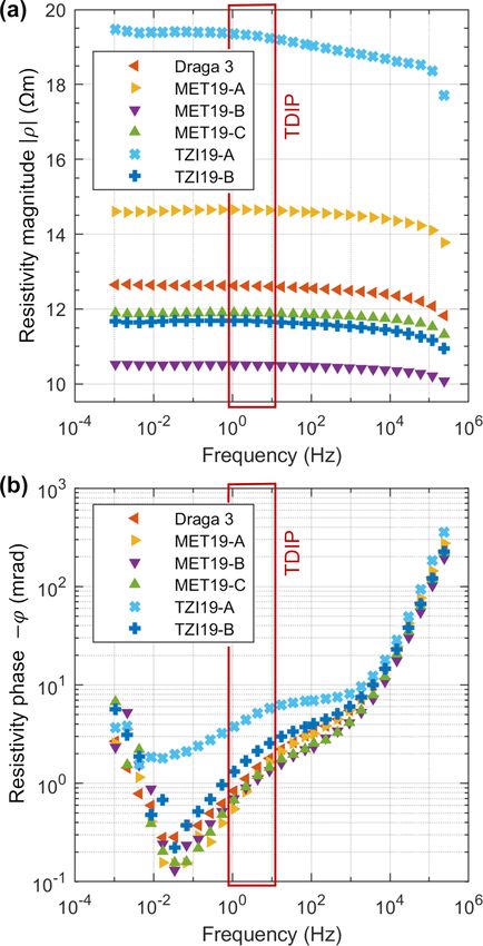
442                                     M. Bücker et al.: Integrated land and water-borne geophysical surveys on karst lakes

                                                                         cations for laboratory analyses (see sampling locations in
                                                                         Fig. 2a and b). On the dry lake bottom, sediment samples
                                                                         were collected using a small spade, whereas an Ekman grab
                                                                         sampler was used to retrieve sediment samples from water-
                                                                         covered areas. Sediment samples were stored in sealed plas-
                                                                         tic bags in order to prevent the loss of moisture; water sam-
                                                                         ples were stored in plastic bottles. All samples were kept cool
                                                                         during transport and storage in order to prevent an increased
                                                                         degradation of organic matter. The electrical conductivity of
                                                                         the water samples (at 20 ◦ C) was measured with a laboratory
                                                                         probe. The frequency-dependent complex electrical resistiv-
                                                                         ity of the samples was measured using a Chameleon I mea-
                                                                         suring device (Przyklenk et al., 2016) in the frequency range
                                                                         from 1 mHz to 240 kHz. To this end, the unconsolidated sed-
                                                                         iments were filled into four-point measuring cells with non-
                                                                         polarizing potential electrodes as used by Kruschwitz (2007)
                                                                         and Bairlein et al. (2014). Prior to and during the measure-
                                                                         ment, the measuring cell was stored in a climate chamber
                                                                         to keep the sample at a constant temperature of 20 ◦ C. Mea-
                                                                         surements were repeated over a period of 4 to 5 d after filling
                                                                         the cell and inserting it into the climate chamber in order to
                                                                         assure equilibrium conditions in the sample. Measurements
                                                                         on relatively dry samples (MET19-A and TZI19-A) resulted
                                                                         in comparably high phase values. These samples were re-
                                                                         moved from the measuring cell, saturated with water of the
                                                                         corresponding lake (using one of the two water samples), and
                                                                         filled again into the measuring cell. This procedure led to
                                                                         more consistent phase measurements compared to the other
                                                                         samples.

                                                                         3.2   Collection of sub-bottom profiler (SBP) lines

                                                                         Low-frequency echo-sounders, often referred to as sub-
                                                                         bottom profilers, are single-channel seismic reflection sys-
                                                                         tems, which are used to obtain bathymetric profiles and pro-
Figure 2. Layout of the geophysical survey on lakes Metzabok
                                                                         vide a high-resolution stratigraphic display of the uppermost
(a) and Tzibaná (b) in October 2019 (after the sudden lake-level         sediments (e.g., Dondurur, 2018). In March 2018, SBP lines
drop) including sub-bottom profiler (SBP), transient electromag-         were collected with the 10 kHz transducer StrataBox HD
netic (TEM), time-domain induced polarization (TDIP), and seis-          (SyQwest), which has an output power of 300 W, mounted
mic refraction tomography (SRT) measurements. The geophysical            on a motor boat. Data were recorded with a record length of
measurements discussed here are grouped into six profiles; black         200 ms and a 1024 Hz sampling frequency. The SBP device
triangles next to the profile names indicate the profile orientations.   was mounted mid-ship in a side mount configuration, with
Yellow and blue triangles indicate sampling locations for sediment       the transducer positioned at 0.4 m below the water surface.
and water samples analyzed in the laboratory, respectively. The          Prior to each survey, the acoustic wave velocity profiles of
dashed black line in (b) indicates the dry part of the river delta ex-   the water columns of the two studied lakes were measured
posed during October 2019.
                                                                         with a Digibar S (Odom Hydrographic). SBP lines were laid
                                                                         out in a regular NS- and EW-oriented grid with separations
TDIP measurements directly on the dry lake bottom (Fig. 2a               of 100 and 300 m, respectively (see Fig. 1b). Navigation data
and b).                                                                  were measured with a differential GPS and stored along with
                                                                         the SBP data.
3.1   Electrical resistivity measurements in the                            During processing, the SBP acoustic traces were read in
      laboratory                                                         using code provided by Kozola (2011) and visualized us-
                                                                         ing a MATLAB script available with this paper. The aver-
In October 2019, a total of six surface sediment samples (top            age value of the acoustic wave velocity of the water column
10 cm) and two water samples were collected at different lo-             (1486.6 m s−1 for both lakes) was used to convert the two-

Solid Earth, 12, 439–461, 2021                                                               https://doi.org/10.5194/se-12-439-2021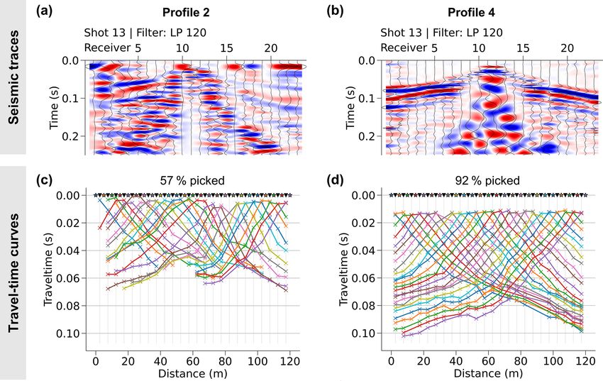
M. Bücker et al.: Integrated land and water-borne geophysical surveys on karst lakes                                             443

way travel time of the acoustic pulse into a depth scale for         bedrock not covered by conductive sediments), constraining
the seismic profiles.                                                the resistivity of the water layer significantly improved the
                                                                     imaging results. Multidimensional effects, as investigated in
3.3   Transient electromagnetic (TEM) soundings                      detail by Mollidor et al. (2013) for TEM data from a lake with
                                                                     steep bathymetric slopes, were not considered in the inter-
TEM soundings were carried out from the water surface us-            pretation as the bathymetric variation along our survey lines
ing a single-loop configuration in March 2018. The loop with         was relatively gentle. Following the approach by Yogeshwar
a diameter of 22.9 m (surface area: ∼ 412 m2 ) consisted of a        et al. (2020), which is based on the one by Spies (1989), we
single, insulated copper wire attached to a floating ring made       estimate the depth of investigation of our TEM soundings
of 24 PVC tubes (diameter 1 in). The ring was towed by an            based on transmitter area and current, average subsurface re-
inflatable boat equipped with an electric motor, which was           sistivity (of the smooth models), and late-time induced volt-
only turned on for navigation between sounding sites. Dur-           age.
ing the measurements, the loop was separated by 5 m from
the inflatable boat. Depending on the specific wind condi-           3.4   Time-domain induced polarization (TDIP)
tions, the unanchored system slowly drifted during the mea-
surements resulting in maximum displacements of approxi-             Time-domain induced polarization (TDIP) data were ac-
mately 2 times the loop diameter (i.e., ∼ 40 m). Due to the          quired with a SyscalPro Switch 48 device (IRIS Instruments)
comparably low measurement velocity (ca. 3 min per sound-            using 48 stainless-steel electrodes separated by 5 or 10 m
ing) and the poor maneuverability of the experimental setup,         depending on the target. The soft and wet mud on the ex-
TEM data were acquired along a limited number of irregu-             posed lake bed provided a good contact between the elec-
larly distributed lines of interest (Fig. 2a).                       trodes and the ground. Where TDIP profiles crossed lime-
   A simple echo-sounder (Garmin Fishfinder series) was              stone outcrops, electrodes were inserted into sediment-filled
used to measure the water depth at each sounding site. A             fractures in order to keep contact resistances as low as pos-
TEM-FAST48 (manufactured by Applied Electromagnetic                  sible. Measurements were carried out with injection currents
Research) was used for the acquisition of TEM sounding               between 0.5 and 1 A, one single stack and a 50 % duty cy-
data. Transients were recorded using a transmitter current           cle with 500 ms pulse length (i.e., duration of off time is also
of 1 A and 32 time gates between 3.6 and 1024 µs after cur-          500 ms). After an initial delay of 20 ms after current shut-off,
rent shut-off. For this transient length, the measuring device       the voltage decay was sampled in 20 time windows with a
records 64 transients, which are analogously averaged by the         constant length of 20 ms. We used a dipole–dipole configu-
hardware. For one sounding measurement, this basic measur-           ration combining short dipole lengths of one electrode spac-
ing cycle is repeated n × 13 times. For n = 4, which we used         ing for superficial measurements with longer dipole lengths
for our measurements, this results in 52 repetitions of the ba-      of 2 and 4 times the electrode spacing for moderate and large
sic cycle and a total of 3328 effective stacks, which are used       depths, respectively. To prevent loss of data quality due to
to compute the impulse response by digital averaging and to          remnant electrode polarization (e.g., Dahlin et al., 2002), the
determine the measurement error as the standard error of the         measurement protocol avoids potential readings using elec-
mean (SEM). For times around 200 µs (the latest time gates           trodes that had been used as current electrodes before (Flo-
used for the inversion), the SEM is 5×10⁻⁹ V Am−2 . For ex-          res Orozco et al., 2012, 2018a). TDIP lines of varying length
emplary TEM data and errors, see Fig. A1 of the Appendix.            were laid out along (and parallel to) selected 2018 SBP and
   During the processing, all transients were truncated to           TEM lines on both lakes (Fig. 2a and b). In order to cover
times from 21.4 and 174.5 µs and inverted using the soft-            the full length of the north–south-running SBP line L4 NS,
ware ZondTEM1d (Alex Kaminsky, personal communi-                     TDIP lines MET19-1 and MET19-2 were carried out as a
cation, 2020). A conventional 1D smoothness-constrained              roll-along profile with an electrode spacing of 10 m and an
modeling approach was used to obtain a one-dimensional               overlap of 12 electrodes.
multilayer model (20 layers) for each sounding position sepa-           During the processing, we removed erroneous measure-
rately. ZondTEM1d supports arbitrarily shaped loops, whose           ments defined as those associated with negative appar-
vertices can be defined independently for transmitter and re-        ent resistivity and/or integral chargeability readings (Flores
ceiver to ensure the correct interpretation of the coincident-       Orozco et al., 2018b). After the removal of erroneous mea-
loop data. The same software was also used to adjust lay-            surements, raw-data pseudo-sections were inspected and ad-
ered models (five layers). In both cases (smooth and layered         ditional outliers were defined as those readings with inte-
model), the water depth measured with the echo-sounder was           gral chargeability values above 8 mV V−1 . Based on an ex-
used as a priori information by fixing the thickness of the          emplary data set, this processing approach is further dis-
first layer to this value. The electrical resistivity of the water   cussed the Appendix. Integral chargeability values were then
layer was fixed to 25 m. This value was manually adjusted           linearly converted to frequency-domain phase shifts assum-
to provide a good overall fit for all soundings. Especially for      ing a constant phase angle response (i.e., no frequency de-
sites with shallow-water depths and a resistive lake bed (i.e.,      pendence) following the approach outlined by Van Voorhis

https://doi.org/10.5194/se-12-439-2021                                                            Solid Earth, 12, 439–461, 2021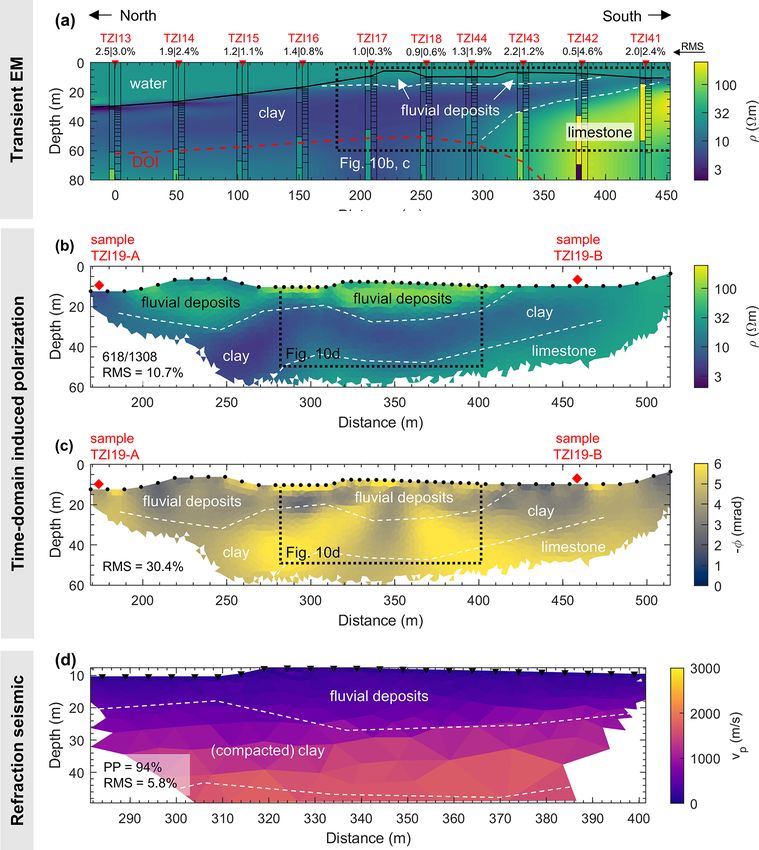
444                                 M. Bücker et al.: Integrated land and water-borne geophysical surveys on karst lakes

et al. (1973) and implemented by Kemna et al. (1999). Fi-
nally, 2D complex-resistivity sections were reconstructed
from the filtered data using the smoothness-constrained least-
squares algorithm CRTomo (Kemna, 2000). 2D sections are
only visualized down to an estimated depth of investigation
by blanking model cells with cumulated sensitivity values
2 orders of magnitude smaller than the maximum cumulated
sensitivity (i.e., the sum of absolute, data-error weighted
sensitivities of all considered measurements; e.g., Weigand
et al., 2017).

3.5    Seismic refraction tomography (SRT)

SRT data were acquired with the 24-channel seismograph
Geode (Geometrics) and 24 28 Hz geophones installed along
a line at 5 m spacing in October 2019. To generate the seismic
signal, a 7.5 kg sledgehammer hitting a steel plate was used
at 25 shot points between the geophone positions as well as
at distances of 2.5 m from the first and last geophone, respec-
tively. At each shot point, five shots were stacked to improve
the signal-to-noise ratio. Due to the limited length (115 m be-
tween the first and the last geophone) and investigation depth,
SRT data were only collected in the central parts of selected
TDIP profiles (Fig. 2a and b).
    During the processing, we applied a 120 Hz low-pass fil-
ter on the seismic traces to remove high-frequency noise and
allow for a more accurate picking of first break travel times.
A tomographic inversion scheme then determines the two-
dimensional velocity structure below the SRT profile based
on the first-arrival travel times (e.g., White, 1989). For the
filtering of the seismic traces and picking of the first ar-
rivals, we used a Python toolbox developed at the TU Wien.
                                                                  Figure 3. Frequency-dependent complex resistivity of six lake-
The observed travel times were inverted with the pyGIMLi          bottom sediment samples retrieved from Lake Metzabok (triangles)
framework (Rücker et al., 2017) following a smoothness-           and Lake Tzibaná (crosses). Complex-resistivity values are given in
constrained scheme. Based on the ray paths computed for           terms of (a) magnitude and (b) phase. The highlighted frequencies
the resolved velocity model (e.g., Ronczka et al., 2017), we      between 1 and 10 Hz roughly correspond to the range tested by our
also determine the so-called ray coverage, which permits the      time-domain induced polarization measurements in the field.
depth of investigation to be illustrated by blanking models
cells that are not covered by any ray.
                                                                  frequency range. We attribute the atypical behavior of the
4     Results and interpretation                                  sample TZI19-A to its fluvial nature (coarse grains and high
                                                                  organic content), while the remaining samples are clearly la-
4.1    Laboratory measurements – electrical properties of         custrine (fine grains and lower organic content). The elevated
       sediment and water samples                                 phase values at high (> 1 kHz) frequencies, which can be ob-
                                                                  served for all six samples, are typical electromagnetic cou-
The complex-resistivity measurements on the six sediment          pling effects (Pelton et al., 1978) but do not affect our TDIP
samples carried out in the laboratory (Fig. 3a) show that         measurements, due to the long initial delay before the sam-
most resistivity values vary within a relatively narrow range     pling of the voltage decay starts.
between 10 and 15 m. Only the resistivity of one sample             The resistivity of the two water samples from the remain-
(TZI19-A) from the river delta in Lake Tzibaná reached val-       ing water bodies used to improve the readings of two dry
ues between 18 and 20 m. Figure 3b shows that phase val-         samples (MET19-A and TZI19-A) were 11.9 m (Metz-
ues (here −ϕ) in the frequency range from 1 to 10 Hz, which       abok) and 26.8 m (Tzibaná), respectively. They are signifi-
is mainly tested by our TDIP measurements, roughly range          cantly lower than the average water resistivity of ∼ 34.5 m
between 0.5 and 4 mrad. Again, the only exception is sample       reported by Rubio Sandoval (2019) for water samples col-
TZI19-A with phase values of up to 6 mrad in the relevant         lected from Lake Metzabok during high lake-level stands in

Solid Earth, 12, 439–461, 2021                                                          https://doi.org/10.5194/se-12-439-2021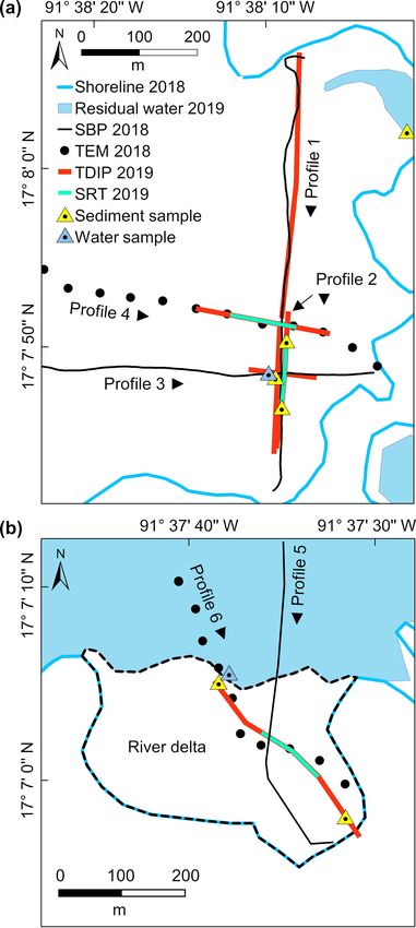
M. Bücker et al.: Integrated land and water-borne geophysical surveys on karst lakes 445
2016. This reduction of electrical resistivity (i.e., increase in fractured and dissolved limestone. Particularly in the flat ar-
conductivity) is probably due to the larger effect of evapora- eas, the sediment cover might also be underlain by blocks
tion on the salinity of small (and shallow) water bodies. In- of collapsed limestone with sediment filling the spaces be-
deed, the remaining water body in Lake Metzabok was much tween blocks and debris. The lakes of the study area show all
smaller (∼ 50 m2 ) than the one in Lake Tzibaná (∼ 5000 m2 ). characteristics of karst lakes, which are expected to originate
However, a comprehensive understanding of the strong varia- from collapsed karst cavities, and the collapse debris should
tion of water conductivity with respect to both sampling loca- still be present below the sediment cover.
tion and time is the subject of ongoing limnological research The electrical images obtained from the co-located TDIP
in the study area. line support this interpretation. The resistivity image (Fig. 4f)
The average resistivity of the sediment samples for the fre- shows a gross separation into two main units: the (i) sed-
quency range between 1 and 117 Hz (and excluding sample iments as well as the supposed limestone debris–sediment
TZI19-A) is 12.25 m, which is typical for saturated clayey mixture stand out with low resistivity values between 10 and
sediments (e.g., Reynolds, 2011). Note that due to the contri- 20 m, while the (ii) limestone outcrops and the deep part
bution of surface conduction along the charged clay-mineral of the section are characterized by higher resistivity values
surfaces (Waxman and Smits, 1968), the bulk resistivity of of up to 300 m. The phase image (Fig. 4g) also shows a
the sediments is even lower than the average resistivity of the separation into units with low and intermediate phase values.
water (25–35 m during high lake-level stands). In our case, Here, a much thinner top layer (compared to the conduct-
this resistivity contrast between lake water and sediments by ing layer in Fig. 4f) stands out with phase values between 0
a factor of 2 to 3 is of particular relevance as it allows us, and 5 mrad, while the limestone bedrock shows phase val-
in principle, to detect the two materials as separate units. To ues > 5 mrad. The capability to separate the pure sediments
our best knowledge, this is the first time that the phase spec- from the limestone–sediment mixture underlines the benefit
tra of fresh lake-bed sediments have been measured in the of evaluating the TDIP phase. Due to the relatively low data
laboratory. cover after outlier removal for large dipole separations, we
do not interpret the phase values at depths > 50 m.
4.2 Field measurements on Lake Metzabok For the sediment infill, both the resistivity values of 10–
20 m and the phase values below 5 mrad are in agreement
In October 2019, Lake Metzabok (average depth 15 m) was with our laboratory measurements on the sediment samples
completely dry, except for some residual ponds. Its sediment- of Lake Metzabok, corresponding to an average resistivity
covered bottom is mostly flat with steep walls (> 50 % slope) of ∼ 12 m and phase values (here −ϕ) < 4 mrad. In con-
and some cliffs along the shore line (Fig. 4a). Only some trast, resistivity and phase values associated with the lime-
drainage channels, steep limestone hillocks, and small ponds stone bedrock are significantly higher than those of the fine-
(Fig. 4a–d) eventually disrupt the smooth lake-bottom topog- grained sediment cover. The intermediate layer, which we in-
raphy. terpret as mixture of fine-grained sediments and the collapse
debris, seems to inherit the low resistivity of the supposed
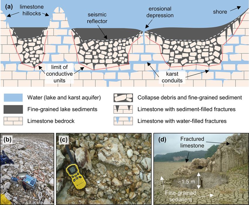
4.2.1 Profile 1 – SBP and TDIP results reveal three clay-rich matrix, while the phase or polarization response is
distinct geological units increased by the limestone debris.
The north–south-oriented SBP line on Profile 1 crosses a 4.2.2 Profile 2 – SRT measurements confirm the
number of these limestone hollocks and depressions, which presence of three geological units identified in the
are well resolved by the first reflector in the seismogram TDIP images
(Fig. 4e). Within the depressions between the limestone out-
crops, a second reflector can be resolved, the geometry of The north–south-oriented Profile 2 runs parallel to the last
which shows a certain consistency with the surface of the part of Profile 1 but is shifted ∼ 10 m east. It is centered at
limestone outcrops. This reflector can be interpreted as the the small pond (Fig. 4d) and has a smaller electrode spac-
lower limit of the sediment cover. The SBP data show that ing (5 m instead of 10 m) to better resolve the sediment-
not only the elevations (outcrops) but also the depressions in limestone contact below the bottom of the pond. The elec-
the sediment cover are influenced by the topography of the trical images (Fig. 5a and b) show the same characteristics as
underlying limestone: both depressions, the drainage chan- seen in the corresponding part of Profile 1. Due to the higher
nel in the northern as well as the small pond in the south- resolution, here, we observe an internal layering of the shal-
ern part, are associated with local risings of the limestone low conductive units with a less conductive (30–50 m) top
surface. Based on the SBP images, the sediment thickness layer of ∼ 10 m thickness and a more conductive (< 20 m)
mostly varies between 5 and 7 m along Profile 1. layer that extends down to 30 m in the northern and southern
Below the surface of the limestone outcrops and the lower parts of the line. The separation into two units becomes more
limit of the sediment cover, respectively, we observe zones obvious in the phase image, where the superficial layer is less
of diffuse reflectivity. These might be related to the heavily polarizable (well below 4 mrad) than the deeper part. A few
https://doi.org/10.5194/se-12-439-2021 Solid Earth, 12, 439–461, 2021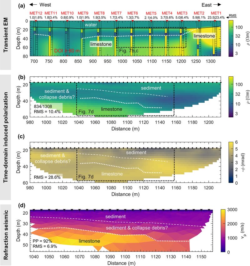
446                                     M. Bücker et al.: Integrated land and water-borne geophysical surveys on karst lakes

Figure 4. Topographic features and geophysical sections along Profile 1 of Lake Metzabok. Photographs taken in October 2019: (a) lake
basin with flat bottom, (b) drainage channel, (c) limestone hillock, (d) deep fracture and pond next to shallow limestone outcrop. (e) Sub-
bottom profiler (SBP) section with dashed lines highlighting the main reflector encountered below the lake floor and dotted lines outlining
a zone of high diffuse reflectivity.(f, g) Electrical resistivity and phase images, respectively, including electrode positions (black dots along
the surface) and dotted lines taken from SBP section. Electrical sections are shifted by 25 m with respect to the SPB section. Labels in the
lower-left corners of (f and g) represent the amount of data points used for the inversion compared to the total measured data (same for
resistivity and phase) and the respective percentage root mean square (RMS) deviations of the inversion.

meters east of the center of the profile, the resistive limestone          gree of fracturing and dissolution of the karst bedrock. The
bedrock crops out, which might explain the significantly in-               seismic velocities of the intermediate layer do not provide
creased resistivity (> 100 m) and phase values (> 6 mrad)                 any additional information on its nature but could well be
over the first 20 m of depth below this part of the profile.               explained by limestone debris or heavily fractured and dis-
   The p-wave velocity structure in the SRT image (Fig. 5c)                solved limestone with sediment-filled open spaces.
confirms the presence of these three units: the shallowest
layer, corresponding with the sediment infill characterized                4.2.3    Profile 3 – comparison of SBP and TDIP
by velocities between 200 and 1000 m s−1 , which is in agree-                       corroborates low phase response of lake
ment with values for unconsolidated fine-grained sediments                          sediments
reported in the literature (Uyanık, 2011); the second layer,
where velocities increase to 1500–2000 m s−1 ; and depths                  The comparison of the SBP line along the west–east-directed
between 15 and 20 m, where a sudden increase to values >                   Profile 3 with the corresponding electrical resistivity images
2500 m s−1 is observed. The p-wave velocities of the deepest               (Fig. 6) confirms the interpretation of the electrical images:
unit agree with the lower limit of typical ranges for limestone            the step in the lower limit of the sediment layer around 490 m
(Reynolds, 2011), which can be explained by the high de-                   along the SBP profile is also reflected in the resistivity struc-
                                                                           ture, and it is clearly resolved in the phase image. Again,

Solid Earth, 12, 439–461, 2021                                                                    https://doi.org/10.5194/se-12-439-2021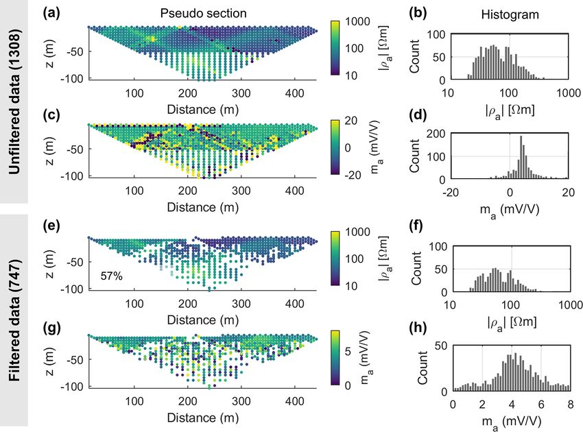
M. Bücker et al.: Integrated land and water-borne geophysical surveys on karst lakes                                                  447

Figure 5. Geophysical sections along Profile 2 of Lake Metzabok (same coordinates as in Fig. 4): (a and b) electrical resistivity and phase
images, respectively, including electrode positions (black dots along the surface), sampling locations of sediment samples (red diamonds
at the surface), and the main lithological units interpreted from the SBP image (dotted lines). Labels in the lower-left corners represent
the amount of data points used for the inversion compared to the total measured data (same for resistivity and phase) and the respective
percentage root mean square (RMS) deviations of the inversion. (c) Seismic refraction tomogram with main lithological units including
picking percentage (PP) and RMS of the inversion.

the conductive unit extends far below the SBP reflector, in             infill across the entire basin. This layer only disappears close
particular between 440–490 m along the profile. We inter-               to the shoreline (i.e., towards the eastern end of the profile),
pret this reflector as the contact between pure sediments and           where the resistive limestone bedrock is in direct contact with
the mixed sediment–collapse debris. Thus, the mixed layer               the water body. According to the layered model, the resis-
has a lower resistivity than the superficial fine-grained sedi-         tive bedrock itself is encountered at depths of approx. 15–
ment layer. Along this profile, both sediment-bearing layers            20 m below the lake bed and only disappears below sounding
are characterized by low phase values. The sediment-covered             MET10, where a possible fracture zone might be responsible
limestone bedrock between 440 and 530 m is characterized                for a lower resistivity at depth.
by high phase values, while phase values decrease as this                  At both ends of the profile, and in particular at stations
unit approaches the surface and crops out at the end of the             MET1 and MET2, a conductor is indicated below the resis-
profile. The low phase values of the limestone outcrop do not           tive bedrock, which could point to a more fractured bedrock
fit the previously stated general characteristics of this unit but      or a lithological contact, e.g., with a shaly geological unit.
might be related to variations in composition and/or degree             However, in the absence of complementary information, such
of fracturing of the limestone bedrock.                                 as a detailed geological map or borehole data, we can also
                                                                        not discard artifacts due to distorted late-time transient data.
4.2.4   Profile 4 – water-borne TEM and terrestrial                     Especially close to the shoreline, where the lake bottom rises
        TDIP measurements reveal consistent resistivity                 steeply, the TEM transients might be affected by multidimen-
        models                                                          sional effects (e.g., Mollidor et al., 2013), which are not taken
                                                                        into account by the chosen one-dimensional inverse model-
Figure 7a shows the electrical resistivity image reconstructed          ing approach.
from 12 TEM soundings along the profile crossing Lake Met-                 Due to the relatively high average resistivity of the sub-
zabok from west to east. Both smooth and layered models                 surface along this profile, the depth of investigation com-
recover a conductive layer of varying thickness below the               puted after Spies (1989) and Yogeshwar et al. (2020) is
lake floor indicating the presence of fine-grained sediment

https://doi.org/10.5194/se-12-439-2021                                                                 Solid Earth, 12, 439–461, 2021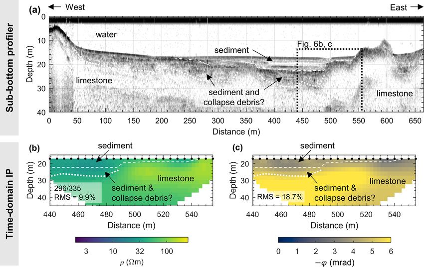
448 M. Bücker et al.: Integrated land and water-borne geophysical surveys on karst lakes
Figure 6. Geophysical sections along Profile 3 of Lake Metzabok: (a) sub-bottom profiler section with dashed lines highlighting the main
reflector found below the lake floor, dotted lines outlining a zone of high diffuse reflectivity including main reflectors and the dashed box
showing the section with TDIP resistivity and phase data; (b) electrical-resistivity image; and (c) phase image including electrode positions
(black dots along the surface) and lines taken from SBP seismogram. Labels in the lower-left corners represent the amount of data points
used for the inversion compared to the total measured data (same for resistivity and phase) and the respective percentage root mean square
(RMS) deviations of the inversion.
mostly larger than the 80 m shown here. Possibly due to the on the assumption that the lakes in the study area are formed
large resistivity and thickness of the limestone bedrock, no by the coalescence of a number of dolines that resulted from
changes of the modeled resistivity have been observed at the collapse of karst cavities. The remains of the collapsed
depths > 80 m. limestone are expected to have formed a debris layer cover-
Between stations MET3 and MET7, the TEM image re- ing the floor of the former caves. Subsequently, the fluvial
covers a resistivity distribution similar to the one of the co- input of fine-grained lake sediments has first filled up the in-
located TDIP profile (Fig. 7b). Taking into account that the terspaces between the blocks and then buried the collapse re-
water-borne TEM survey was carried out with an average of mains, forming the two uppermost units observed below all
15 m water column, the consistency with the TDIP resistivity profiles. Figure 8b and c show pictures of such mixed mate-
results from the lake bed clearly indicates the good quality rials exposed on the surface of the drained Lake Metzabok.
and reliability of the obtained TEM imaging results. Table 1 summarizes the physical properties of the main
As observed before, the phase image (Fig. 7c) shows a units of this geological interpretation. The electrical resis-
non-polarizable top layer, which at a depth of ∼ 10 m is un- tivity of the fine-grained sediments and the mixed collapse
derlain by a unit with a higher polarization response (abso- debris and sediment layer is comprised within a relatively
lute phase values around 10 mrad and higher), corresponding narrow range. In the TEM and TDIP resistivity images, these
with the debris–sediment unit. The SRT tomogram (Fig. 7d) two units may appear as one conductive unit (see red dotted
shows a sharp increase in p-wave velocity at depths between lines in Fig. 8a). It is not clear why the addition of the more
20 m (in the western part) and 30 m (in the eastern part). This resistive lime stone debris should decrease the resistivity of
southeast-dipping surface correlates with a similar structure the mixed unit compared to the pure fine-grained sediments.
in the TDIP resistivity model, which we again interpret as the In terms of the phase values, the distinction between these
contact with the limestone bedrock. units is clearer and the increase in the phase response in the
mixed layer is straightforward (because the limestone is more
4.2.5 Geological interpretation of the geophysical polarizable than the fine-grained sediments based on our field
survey on Lake Metzabok measurements). The clearest indication of the inner structure
of the conductive unit comes from the collocated SBP sec-
The schematic sketch presented in Fig. 8a summarizes our tions, which show a clear seismic reflector at the correspond-
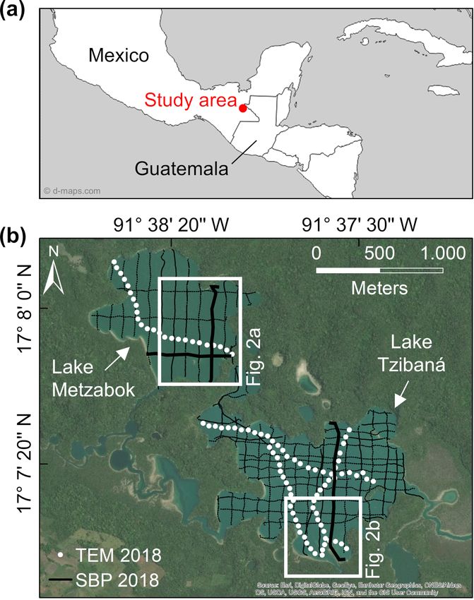
geological interpretation of the geophysical profiles of Lake ing depth. The limestone bedrock becomes detectable by its
Metzabok and the observations made on the exposed bed of high p-wave velocity in the SRT images and its high resistiv-
the drained lake (Figs. 4a–d and 8b and d). The model rests
Solid Earth, 12, 439–461, 2021 https://doi.org/10.5194/se-12-439-2021M. Bücker et al.: Integrated land and water-borne geophysical surveys on karst lakes 449
Figure 7. Geophysical sections along Profile 4 of Lake Metzabok: (a) interpolated TEM image based on smooth 1D models; left bar
graphs show layered, right bar graphs smooth models, and individual percentage RMS deviations are given for layered and smooth models,
respectively. The black solid line in the section indicates the water–sediment contact, the dotted line the top of the limestone bedrock inferred
from this image. (b) Electrical resistivity and (c) phase images including electrode positions (black dots along the surface), and the main
lithological units as interpreted from the SRT image in (d) (dotted lines). Labels in the lower-left corners of (b) and (c) represent the amount
of data points used for the inversion compared to the total measured data (same for resistivity and phase) and the respective percentage RMS
of the inversion. (d) Seismic refraction tomogram with main lithological units including picking percentage (PP) and RMS of the inversion.
ity (TEM and TDIP), while its phase response varies over a along the shoreline and flat parts with the typical three-layer
larger range and is not as unambiguous. It is worth mention- structure consisting of fine-grained sediment cover, collapse
ing that wherever the fine-grained sediments are underlain debris, and limestone bedrock. Unlike in the case of Lake
by the collapse-debris layer, the limestone bedrock does not Metzabok, the flat parts of Lake Tzibaná are found at two
appear as an additional reflector in the SBP sections. different levels, which are separated from one another by a
steep limestone cliff. Additionally, the southern part of the
4.3 Field measurements on Lake Tzibaná profile crosses the delta of the Nahá river, where we expect
a higher fraction of coarser material (sand and gravel) in the
fluvial deposits in comparison to the well sorted sediments,
While the 2019 lake-level decrease left Lake Metzabok (max.
mainly composed of clay and silt, covering the flat parts of
depth 25 m) completely drained, the deeper Lake Tzibaná
the lake bottom. In the SBP profile, these delta deposits stand
(max. depth 70 m) always preserved a water cover on at
out by a highly reflective lake bottom, which results in strong
least two-thirds of its maximum surface area. The long N–
multiple reflections between lake bottom and water surface.
S-oriented SBP section in Fig. 9 crossing the entire Lake Tz-
Yet, such reflections inhibit the recovery of any information
ibaná (Profile 5) shows a similar lake-bottom architecture to
on the internal structure of the delta.
the one derived for Lake Metzabok: steep limestone walls
https://doi.org/10.5194/se-12-439-2021 Solid Earth, 12, 439–461, 2021450 M. Bücker et al.: Integrated land and water-borne geophysical surveys on karst lakes
Figure 8. (a) Schematic sketch summarizing the geological conditions below Lake Metzabok interpreted from the geophysical survey (details
not drawn to scale). The limit between the fine-grained lake sediments and the collapse debris with sediment-filled interspaces indicated by
the white dashed line stands out as a strong reflector in all sub-bottom profiler images. All units containing fine-grained sediment are
characterized by low electrical resistivity values; a strong resistivity increase marks the upper limit of the limestone bedrock as indicated by
the red dotted line. Photographs show (b and c) limestone debris with fine-grained sediment as well as (d) fractured limestone and fine lake
sediments exposed during the low-level stands in October 2019.
Table 1. Ranges of physical properties of the geological units interpreted from our geophysical profiles and laboratory measurements.
Resistivity data based on TEM, TDIP resistivity, and laboratory measurements. Phase data (absolute value) according to TDIP images and
laboratory data between 1 und 10 Hz; p-wave velocity from SRT images.
Material/geological unit Resistivity Phase p-Wave velocity
(m) (mrad) (m s−1 )
Fine-grained sediments 5–30 5–6 1500–2000
Limestone bedrock > 100 > 4–5 > 2000
The TEM, TDIP, and SRT measurements carried out along TZI41 indicates a conducting unit below the resistive lime-
Profile 6, which roughly covers the last 450 m of Profile 5 stone bedrock, which could be related to a lithological con-
(see survey layout in Fig. 2b), fill in this missing informa- tact, a fracture zone, distorted late-time data, or multidimen-
tion. The resistivity images of both TEM and TDIP measure- sional effects. The low average resistivity below soundings
ments presented in Fig. 10a and b consistently show three TZI13–44 result in a significantly reduced depth of inves-
main units: (1) the resistive (> 100 m) limestone bedrock at tigation (approx. 55–60 m). The lack of borehole data hin-
depth, (2) a highly conductive (< 10 m) clay layer on top, ders a conclusive interpretation of this conductive anomaly
and (3) a layer of intermediate resistivity (∼ 30–100 m), at depth.
in particular between 200 and 400 m, corresponding to the Probably due to the highly heterogeneous composition of
sand banks and possible interbedded strata of clay, sand, the river delta, these deposits also show a heterogeneous dis-
and gravel associated with the delta deposits. As observed tribution of phase values (Fig. 10c). As observed before, the
above along Profile 4, the resistivity model of TEM sounding clay and limestone units below the fluvial deposits show low
Solid Earth, 12, 439–461, 2021 https://doi.org/10.5194/se-12-439-2021M. Bücker et al.: Integrated land and water-borne geophysical surveys on karst lakes 451
Figure 9. Long N–S-oriented sub-bottom profiler section crossing the entirety of Lake Tzibaná (Profile 5). The last approx. 450 m roughly
coincides with the TEM section along Profile 6 in Fig. 10a (indicated by the dotted rectangle). The white dashed lines highlight the main
reflector below the lake floor, which is interpreted as the lower limit of a fine-grained sediment layer. The white dotted lines enclose the
zone of diffuse reflectivity associated with the collapsed, sediment-filled limestone. The black dashed line indicates the approximate lake
level during the second field season in October 2019. The last 500 m of the profile correspond to the delta of the Nahá river, where a high
reflectivity of the sand-covered lake floor results in the occurrence of strong multiples in the seismogram.
and high phase values, respectively. The relatively high phase erably higher, due to the larger water column at this location
values in the clay layer below the fluvial deposits are prob- (approx. 30 m during water-level high stand in 2019).
ably inversion artifacts caused by the relatively noisy TDIP With a thickness of > 40 m according to our electrical
data along this line. imaging results, the sedimentary cover along Profile 5 of
The SRT image (Fig. 10d) shows p-wave velocities as low Lake Tzibaná (particularly between 250 and 400 m) is much
as 100–200 m s−1 within the fluvial deposits, which are in thicker than the sediments covering the flat parts of both
agreement with literature values for partially saturated, un- lakes. However, our results also indicate that these sediments
consolidated sand (e.g., Barrière et al., 2012). The p-wave rather correspond to fluvial deposits of the river delta. In this
velocities increase with depth across the thick (and proba- depositional regime, we expect much higher rates of sedi-
bly compacted) clay layer. According to the electrical im- mentation and thus not necessarily an older paleoenviron-
ages, the surface of the bedrock lies below the lower limit mental record. Additionally, river deltas are much more dy-
of the SRT image. Accordingly, the highest velocities of namic systems, in which sediments are deposited, eroded,
< 2000 m s−1 , seen in the SRT image, do not reach the high and redeposited repeatedly, which decreases the probability
values (> 2500 m s−1 ) typical for limestone bedrock. to obtain undistorted sediment records as encountered farther
offshore.
5 Discussion
5.2 Geological situation of the studied lakes and
5.1 Identification of suitable drilling locations hydrogeological implications
Our geophysical investigations delineate a 5–6 m thick and Our field observations and geophysical imaging results also
nearly undisturbed layer of fine-grained lacustrine sediments have important implications for the general understanding
covering the flat parts of Lake Metzabok. Such a layer is rel- of the geological situation of the two studied karst lakes:
evant for the conduction of paleolimnological perforations. large areas of both lakes are covered by a layer of clayey
Suitable drilling locations can be defined between 450 and sediments, which have a low hydraulic permeability. Thus,
550 m, as well as between 600 and 700 m along Profile 1 where this layer is thick enough (up to 5–6 m across large ar-
(SBP profile in Fig. 4e). The large variation of the sedi- eas), it acts as a hydrological barrier between the lakes and
ment thickness observed along Profile 3, which is perpen- the underlying karst. However, the remaining heavily frac-
dicular to Profile 1, underlines the need for a comprehen- tured and uncovered limestone outcrops (e.g., Fig. 8b–d) ef-
sive pre-drilling investigation and an accurate positioning of fectively connect the lakes with the karst water system. This
the drilling equipment. The sediment layer between 100 and conclusion is underscored by the high velocity at which the
200 m along Profile 5 represents a suitable drilling location two lakes drained practically simultaneously between Febru-
for Lake Tzibaná (sediment thickness also 5–6 m). Although ary and July 2019. Accordingly, the sudden drainage of both
the deeper part of Lake Tzibaná is covered by sediments (be- lakes might be related to the same hydrogeological process.
tween 400 and 600 m along Profile 5), too, sediment thick- While the interconnectivity between surface water and
nesses in this part of the lake are smaller (only 3–4 m accord- karst aquifer is well documented by field observations and
ing to the SBP image) and drilling efforts would be consid- further supported by the interpretation of our geophysical re-
https://doi.org/10.5194/se-12-439-2021 Solid Earth, 12, 439–461, 2021452 M. Bücker et al.: Integrated land and water-borne geophysical surveys on karst lakes
Figure 10. Geophysical sections along Profile 6 of Lake Tzibaná: (a) interpolated TEM image based on smooth 1D models; left bar graphs
show layered, right bar graphs smooth models, and individual percentage RMS deviations are given for layered and smooth models, respec-
tively. The black solid line indicates the water–sediment contact, the dashed line the main lithological contacts inferred from this image.
(b) Electrical resistivity and (c) phase images including electrode positions (black dots along the surface) and main lithological units. Red
diamonds on the surface indicate the location of the sediments sampled for laboratory analyses. Labels in the lower-left corners of (b) and
(c) represent the amount of data points used for the inversion compared to the total measured data (same for resistivity and phase) and the
respective percentage root mean square (RMS) deviations of the inversion. (d) Seismic refraction tomogram including picking percentage
(PP) and RMS of the inversion, contacts of main lithological units (white dashed lines) taken from TDIP resistivity image.
sults (see Fig. 8), the specific cause(s) and mechanism(s) of 5.3 Lessons learned from implementing a
the sudden drainage of Lakes Metzabok and Tzibaná remain multi-methodological approach for lake-bottom
unrevealed. The suddenness of the drainage suggests that one reconnaissance
or more previously clogged karst conduits were unplugged
around these dates. Planned time-series analyses of hydro-
logical and meteorological data in combination with paleoen- Only the combination of complementary methods employed
vironmental studies on sediment cores will possibly provide in the present study allowed us to produce comprehensive
more detailed insight into the mechanism and its triggers and geological models of the lake-bottom geology of the studied
thus shed light on the question of whether such catastrophic karst lakes. Table 2 summarizes the characteristics of the four
drainage events as the one observed during 2019 are linked field methods (SRT, TEM, TDIP, and SRT), the individual
to recent climate change or another geodynamic process. contributions of each method, and their respective limitations
identified in this study. In the following, we will discuss some
important aspects of this overview in more detail.
Solid Earth, 12, 439–461, 2021 https://doi.org/10.5194/se-12-439-2021You can also read