Towards end-to-end (E2E) modelling in a consistent NPZD-F modelling framework (ECOSMO E2E_v1.0): application to the North Sea and Baltic Sea - GMD
←
→
Page content transcription
If your browser does not render page correctly, please read the page content below
Geosci. Model Dev., 12, 1765–1789, 2019
https://doi.org/10.5194/gmd-12-1765-2019
© Author(s) 2019. This work is distributed under
the Creative Commons Attribution 4.0 License.

Towards end-to-end (E2E) modelling in a consistent NPZD-F
modelling framework (ECOSMO E2E_v1.0): application to the
North Sea and Baltic Sea
Ute Daewel1 , Corinna Schrum1,2 , and Jed I. Macdonald3,4
1 Helmholtz  Centre Geesthacht, Institute of Coastal Research, Max-Planck-Str. 1, 21502 Geesthacht, Germany
2 Geophysical  Institute, University of Bergen, Allegaten 41, 5007 Bergen, Norway
3 Faculty of Life and Environmental Sciences, University of Iceland, 101 Reykjavík, Iceland
4 Oceanic Fisheries Programme, Pacific Community (SPC), Noumea BP D5 98848, New Caledonia

Correspondence: Ute Daewel (ute.daewel@hzg.de)

Received: 24 September 2018 – Discussion started: 21 November 2018
Revised: 14 March 2019 – Accepted: 10 April 2019 – Published: 6 May 2019

Abstract. Coupled physical–biological models usually re-            period. Additionally, we performed scenario tests to analyse
solve only parts of the trophic food chain; hence, they run         the new role of the zooplankton mortality closure term in the
the risk of neglecting relevant ecosystem processes. Addi-          truncated NPZD and the fish mortality term in the end-to-end
tionally, this imposes a closure term problem at the respec-        model, which summarises the pressure imposed on the sys-
tive “ends” of the trophic levels considered. In this study,        tem by fisheries and mortality imposed by apex predators.
we aim to understand how the implementation of higher                  We found that the model-simulated macrobenthos and fish
trophic levels in a nutrient–phytoplankton–zooplankton–             spatial and seasonal patterns agree well with current system
detritus (NPZD) model affects the simulated response of             understanding. Considering a dynamic fish component in the
the ecosystem using a consistent NPZD–fish modelling ap-            ecosystem model resulted in slightly improved model perfor-
proach (ECOSMO E2E) in the combined North Sea–Baltic                mance with respect to the representation of spatial and tem-
Sea system. Utilising this approach, we addressed the above-        poral variations in nutrients, changes in modelled plankton
mentioned closure term problem in lower trophic ecosystem           seasonality, and nutrient profiles. Model sensitivity scenarios
modelling at a very low computational cost; thus, we provide        showed that changes in the zooplankton mortality parame-
an efficient method that requires very little data to obtain spa-   ter are transferred up and down the trophic chain with little
tially and temporally dynamic zooplankton mortality.                attenuation of the signal, whereas major changes in fish mor-
   On the basis of the ECOSMO II coupled ecosystem model            tality and fish biomass cascade down the food chain.
we implemented one functional group that represented fish
and one group that represented macrobenthos in the 3-D
model formulation. Both groups were linked to the lower
trophic levels and to each other via predator–prey relation-        1   Introduction
ships, which allowed for the investigation of both bottom-up
processes and top-down mechanisms in the trophic chain of           The majority of spatially resolved marine ecosystem mod-
the North Sea–Baltic Sea ecosystem. Model results for a 10-         els are dedicated to a specific part of the marine food web.
year-long simulation period (1980–1989) were analysed and           These models can be differentiated into lower-trophic-level
discussed with respect to the observed patterns. To under-          nutrient–phytoplankton–zooplankton models (so-called NPZ
stand the impact of the newly implemented functional groups         models or LTL models – e.g. Blackford et al., 2004; Daewel
for the simulated ecosystem response, we compared the per-          and Schrum, 2013; Maar et al., 2011; Schrum et al., 2006;
formance of the ECOSMO E2E to that of a respective trun-            Skogen et al., 2004) and, on the other end of the trophic
cated NPZD model (ECOSMO II) applied to the same time               chain, higher-trophic-level models (HTL models). The lat-

Published by Copernicus Publications on behalf of the European Geosciences Union.
1766                                                                                   U. Daewel et al.: ECOSMO E2E_v1.0

ter mainly simulate fish on the species level, including both     which are often vital for advising ecosystem management,
single-species individual-based models (IBMs; e.g. Daewel         a clear weakness of these models is the huge amount of data
et al., 2008; Megrey et al., 2007; Politikos et al., 2018;        needed for model parameterization (Peck et al., 2015) and
Vikebø et al., 2007) and multi-species models. Although           the sensitivity of the models to assumptions made regard-
some of these models are complex and already include many         ing the food web structure and functioning. Another draw-
food web components such as OSMOSE (Shin and Cury,                back of the recent end-to-end models is the lack of spa-
2004, 2001) and ERSEM (Butenschön et al., 2016), the sep-         tial resolution. They are either solved in 2-D (such as EwE)
aration of trophic levels often constrains such models’ abil-     or are resolved in predefined (based on environmental con-
ity to simulate and distinguish between major control mech-       ditions) larger area polygons (such as Atlantis). This con-
anisms on marine ecosystems (Cury and Shannon, 2004).             sequently excludes the dynamic resolution of ecologically
The difficulty of resolving trophic feedback mechanisms in-       highly relevant hydrographical structures such as tidal fronts
creases the uncertainties when modelling the impacts of ex-       or the thermocline, and it implies that future changes in rele-
ternal controls on the trophic food chain (e.g. Daewel et al.,    vant hydrodynamics and their impacts cannot be considered
2014; Peck et al., 2015).                                         using these models. To our knowledge, the first approach
   In the last 10 to 15 years, major efforts have been made       that attempted to resolve the trophic food web more con-
to link the different trophic levels together to cover the ma-    sistently in a functional group framework with the spatial
rine ecosystem from the lowest to the uppermost “end” (end-       and temporal resolution of a state-of-the-art physical model
to-end: E2E) (Christensen and Walters, 2004; Fennel, 2009;        was the food web model presented by Fennel (2010, 2008)
Fulton, 2010; Heath, 2012; Shin et al., 2010; Travers et al.,     and Radtke et al. (2013). The above-mentioned research
2007; Watson et al., 2014). Although some models such as          proposed a nutrient-to-fish model where fish is consistently
Atlantis (Fulton et al., 2005), StrathE2E (Heath, 2012), and      included in a NPZD (nutrient–phytoplankton–zooplankton–
Ecopath with Ecosim (EwE; Christensen and Walters, 2004)          detritus) model framework using a Eulerian approach. In
consider more trophic levels (from phytoplankton to marine        these studies they chose a species-specific way of introducing
mammals and birds and/or fisheries) consistently within the       fish, using size-structured formulations for the three major
model formulation, the majority of approaches couple con-         fish species in the Baltic Sea. The model has been proven to
ceptually different model types – either “one-way”, with no       work well in the Baltic Sea, which is characterised by a rel-
feedback on the lower trophic levels (e.g. Daewel et al., 2008;   atively simple food web (Casini et al., 2009; Fennel, 2008),
Rose et al., 2015; Utne et al., 2012), or “two-way” (e.g.         but it is likely more difficult to parameterise in other, more
Megrey et al., 2007; Oguz et al., 2008) – when linking the        complex structured food webs involving more key species
trophic levels. All of these approaches work reasonably well      such as those in the North Sea.
in serving a specific purpose or scientific question, but are         Here, we aim to address these conceptual limitations in
accompanied by different uncertainties and conceptual lim-        end-to-end modelling and present a different approach based
itations to model ecosystem structuring under external forc-      on the assumption that food availability and correspond-
ing. While one-way coupled approaches neglect feedbacks           ing energy and mass fluxes are the major controls on the
and therefore imply difficulties at the model interfaces, com-    higher trophic production and spatial and temporal distri-
prehensive food web models like Atlantis resolve food webs        bution of fish biomass. A physical–biological coupled 3-D
on the basis of species or specific groups and are difficult to   NPZD ecosystem model is extended to include fish and mac-
parameterise, especially in complex ecosystems. One of the        robenthos (MB). Although our idea is inspired by the model
most commonly used food web modelling tools is the Eco-           presented by Fennel (2010, 2008) and Radtke et al. (2013),
path with Ecosim (EwE) modelling software (Christensen            it is substantially different to their concept which is based on
and Walters, 2004), which provides an instantaneous snap-         three key species. We used a functional group approach in-
shot of the trophic mass balance in marine food webs. The         stead, which represents the entire fish population and aims
combination of the software’s dynamical modelling capabil-        to be consistent with the functional group approach used
ity (Ecosim) and a tool that replicates the model on a spatial    for phytoplankton and zooplankton. This enables the esti-
grid (Ecospace) allows for 2-D estimates of the system’s re-      mation of the total fish production potential and allows for
sponse to e.g. policy measures. However the approach still        the structuring impacts on the ecosystem to be resolved. The
falls short when simulating ecosystem dynamics at high tem-       advantage of this generic approach is its broad applicability.
poral and 3-D spatial resolutions. In Peck et al. (2015),         It allows for general and comparative studies on changing
a number of different ecosystem models used in the Eu-            ecosystem structure and is not limited by unknown changes
ropean VECTORS project (http://www.marine-vectors.eu/,            in key species for the respective ecosystems. The approach
last access: 2 May 2019) were reviewed. Besides discussing        we use cannot address changes in ecosystem structure related
statistical and physiology-based life cycle models, Peck et       to variations in the fish assemblage or selected fishing activ-
al. (2015) identified strengths and weaknesses in food web        ities. However, it does provide the potential for further de-
models like Atlantis. While the strength of these models          velopments towards a more complex food web (e.g. by dis-
is the explicit consideration of species-specific responses,

Geosci. Model Dev., 12, 1765–1789, 2019                                             www.geosci-model-dev.net/12/1765/2019/
U. Daewel et al.: ECOSMO E2E_v1.0 1767
tributing fish into separate feeding guilds), which will then (Ekeroth et al., 2016) and salinity (Gogina et al., 2010). Be-
allow us to address specific changes in food web structure. sides their role as prey and predator in the marine food web,
We present the first application of a Eulerian end-to-end macrobenthos additionally influences nutrient effluxes from
model for the shelf sea system of the North Sea and the Baltic the sediments and can therefore modify the temporal and spa-
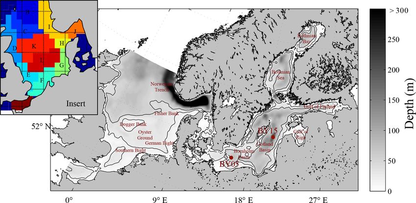
Sea. The coupled North Sea–Baltic Sea system (Fig. 1) is lo- tial patterns of nutrient concentrations (Ekeroth et al., 2016).
cated adjacent to the North Atlantic Ocean. Despite the close Here we present a functional type, E2E modelling ap-
proximity of these seas, they are very different with respect to proach, which relates food availability to potential fish
their physical and biogeochemical characteristics. The North growth and biomass distributions. In this paper we intro-
Sea features pronounced co-oscillating tides combined with duce the conceptual basis of the model, discuss its charac-
a major inflow from the North Atlantic. The Baltic Sea in teristics, and explore its performance with respect to the ob-
contrast, only has a narrow opening to the North Sea which served fish and MB distributions. Furthermore, we analyse
leads to an almost enclosed, brackish system with weak tidal model performance at the lower trophic levels in comparison
forcing (Müller-Navarra and Lange, 2004). The restricted ex- to the NPZD modelling approach, and discuss the potential
change capacity and fresh water excess of the Baltic Sea lead of our model for understanding and comparing basic regional
to an estuarine-type circulation with strong stratification and ecosystem characteristics.
relatively low salinities in addition to a relatively long wa-
ter residence time of about 30 years (Omstedt and Hansson,
2006; Rodhe et al., 2006). Due to its brackish waters, win- 2 Methods
ter sea ice regularly develops in the Baltic Sea, which can,
2.1 Model description
in severe winters, cover almost the entire surface (Seinä and
Palosuo, 1996). The E2E model builds on the coupled hydrodynamic–lower-
The two systems also differ substantially in terms of trophic-level ecosystem model ECOSMO II (Barthel et al.,
ecosystem dynamics. The North Sea is known as a highly 2012; Daewel and Schrum, 2013; Schrum et al., 2006;
productive area inhabited by more than 26 zooplankton taxa Schrum and Backhaus, 1999), which is further expanded
(Colebrook et al., 1984) and over 200 fish species (Daan for the present study. The latter model has been shown to
et al., 1990), with the majority of the biomass distributed accurately reproduce lower-trophic-level ecosystem dynam-
among demersal gadoids, flatfish, clupeids, and sand eel ics in the coupled North Sea–Baltic Sea system. The model
(Ammodytes marinus) (Daan et al., 1990). Consequently, the equations and a model validation on the basis of nutrients
North Sea is economically highly relevant with nine nations were presented in detail by Daewel and Schrum (2013), who
fishing in the area and current landings of about 2 × 10⁶ t showed that the model is able to reasonably simulate ecosys-
annually (ICES, 2018b). Compared with the North Sea, the tem productivity in the North Sea and the Baltic Sea on
species composition in the Baltic Sea is primarily limited seasonal up to decadal timescales. The NPZD module was
by the low salinities and encompasses only a few key zoo- designed to simulate different macronutrient limitation pro-
plankton (Möllmann et al., 2000) and fish (Fennel, 2010) cesses in targeted ecosystems and comprises 16 state vari-
species. Thus, compared to the North Sea, commercial fish- ables. Besides the three relevant nutrient cycles (nitrogen,
ing in the Baltic Sea is limited to a few stocks with total phosphorus, and silica), three functional groups of primary
landings of over 0.6 ×10⁶ t annually (ICES, 2018a). In both producers (diatoms, flagellates, and cyanobacteria) and two
regions, landings peaked in the 1970s and have substantially zooplankton (herbivore and omnivore) groups were resolved.
(ca. 50 %) declined since then. Thus, fishing has a substantial Additionally, oxygen, biogenic opal, detritus, and dissolved
impact on the overall fish biomass in the region. organic matter were considered. Sediment is implemented in
Studies on the food web dynamics of the North Sea and the model as an integrated surface sediment layer, which ac-
Baltic Sea have additionally highlighted the relevance of ben- counts for the consideration of sedimentation as well as re-
thic fauna for fish consumption (Greenstreet et al., 1997; suspension. Biogeochemical remineralisation is considered
Tomczak et al., 2012). The term benthos generally refers to in surface sediments leading to inorganic nutrient fluxes into
all organisms inhabiting the sea floor. A comprehensive re- the overlying water column. To allow for nutrient-specific
view on the topic is given in Kröncke and Bergfeld (2003). processes in the sediment, the organic silicate content of the
The faunal components encompass over 5000 species which sediment is estimated in a separate state variable. A third
are generally divided by size into microfauna, meiofauna, sediment compartment is considered for iron-bound phos-
and macrofauna. Additional differentiation can be made by phorus in the sediment (Neumann and Schernewski, 2008).
considering the vertical habitat structure, with infauna in- To estimate total fish production and biomass in a consis-
habiting the inner part of the sediment and epifauna liv- tent manner compared with lower-trophic-level production,
ing above the sediments. While macrobenthos assemblages we expanded the NPZD-type model via the implementation
in the North Sea are structured based on the spatial distri- of a wider food web in the system (Fig. 2).
bution of sediment characteristics and depth, the Baltic sea
community is additionally influenced by oxygen availability
www.geosci-model-dev.net/12/1765/2019/ Geosci. Model Dev., 12, 1765–1789, 2019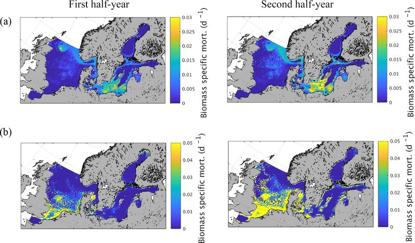
1768                                                                                          U. Daewel et al.: ECOSMO E2E_v1.0

Figure 1. Model area and bathymetry. Black lines indicate depths of 30 and 60 m respectively. The insert represents the area subdivision in
the ICES boxes for model comparison to ICES data (see Fig. 10).

Figure 2. Schematic diagram of biological–geochemical interactions in ECOSMO E2E.

   Although zooplankton in ECOSMO II could in princi-                   compartment in ERSEM (Butenschön et al., 2016), where
ple also grow at the bottom, its parameterization as a pas-             the benthic predators are distributed into three different func-
sive tracer and the choice of parameterization for the func-            tional types, in this study we neglect different functional
tional groups makes it unsuitable for representing benthic              traits of infauna and epifauna and only consider one func-
production. Hence, the parameterisation of a specific func-             tional group, which we, for convenience, will refer to as mac-
tional group representing benthic (meio- and macro-) fauna              robenthos (MB).
remains necessary. The group was designed in a similar fash-               Each state variable C in ECOSMO II is estimated follow-
ion to the zooplankton groups, but with the additional restric-         ing prognostic equations in the form of
tion that benthos only grows at the bottom and is not ex-
posed to advection or diffusion. Benthic fauna has been ob-             Ct + (V · ∇) C + (wd ) Cz = (Av Cz )z + Rc                     (1)
served to exhibit little tolerance to hypoxic and anoxic con-
ditions (Kröncke and Bergfeld, 2003); therefore macroben-               with Ct = ∂C           ∂C
                                                                                    ∂t , Cz = ∂z , where t is time and z is the ver-
thos growth was only estimated for positive oxygen concen-              tical coordinate. The equation includes advective transport
trations in the model framework. In contrast to the benthic             (V · ∇)C(V = (u, v, w) the current velocity vector), verti-
                                                                        cal turbulent sub-scale diffusion (Av Cz )z (Av is the turbulent

Geosci. Model Dev., 12, 1765–1789, 2019                                                    www.geosci-model-dev.net/12/1765/2019/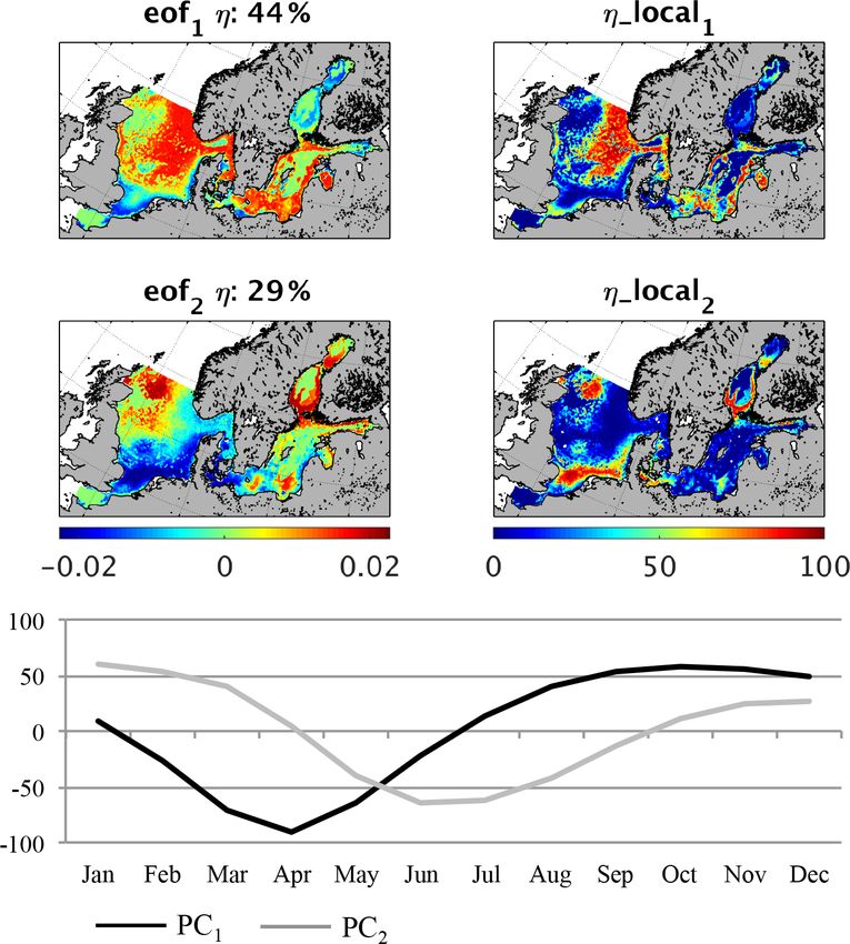
U. Daewel et al.: ECOSMO E2E_v1.0                                                                                                      1769

sub-scale diffusion coefficient), sinking rates (wd )Cz (the wd    Table 1. Parameters used for the MB functional group reaction
sinking rate is non-zero for detritus, opal, and cyanobacteria),   terms.
and chemical and biological reactions (Rc ). As MB produc-
                                                                    Abbreviation     Definition                      Value     Units
tion occurs locally at the bottom and the group is not exposed
to mechanical displacement, Eq. (1) is simplified for MB:           rMB              MB half-saturation constant        0.5    mmol C m−3
                                                                    mMB              MB mortality rate               0.001     d−1
dCMB                                                                εMB              MB excretion rate               0.025     d−1
     = [RMB ]z = zbottom                                    (2)
 dt                                                                 γMB              Assimilation efficiency          0.75
                                                                    σMB,X            Grazing rate                      0.1     d−1
Concurrently chemical and biological interactions are em-
ployed in the biological reaction term RC , which is different
for each variable (C) based on the relevant biochemical pro-       Table 2. Feeding preferences for macrobenthos (MB) and fish (Fi)
cesses. For MB it is divided into production, which is a func-     aY,X .
tion of consumption (RMB_Cons ) and assimilation efficiency
(γMB ), and a MB loss term as follows:                               Y    X    P       Z1         Z2     D         DOM        Sed. 1   MB

RMB = γMB RMB_Cons − RMB_Loss                               (3)      MB        0.2     0.2        0.3    0.1       0.1        0.1      -
                                                                     Fi        –       0.25       0.45   0.05      –          –        0.25
The production of zooplankton in the model depends on the
available food resources, which include phytoplankton, detri-
tus, and (for the omnivorous zooplankton group) also herbiv-         The MB loss term consists of excretion (εMB CMB ), natural
orous zooplankton. For the macrobenthos functional group,          mortality (mMB CMB ), and predation mortality from the fish
we assume a much wider range of potential prey items. The          functional group (CFi GFi (CMB )). Values for excretion (εMB )
benthic community can be divided into the following groups:        and mortality rate (mMB ) are given in Table 1.
benthic suspension-/filter-feeders that mainly feed on phyto-
plankton, detritus, and bacteria; benthic deposit-feeders that     RMB_Loss = CFi GFi (CMB ) + mMB CMB + εMB CMB                         (6)
ingest bottom sediments; and larger individuals that exert
predation pressure (among others) on the available zooplank-       We assume that “fish” is a prognostic variable, which is, in
ton (Kröncke and Bergfeld, 2003). Thus, the prey spectrum          contrast to the other prognostic state variables in the ecosys-
of the simulated MB functional group also includes, besides        tem model, not exposed to passive transport processes and
phyto- and zooplankton, detritus, and organic sediments. As        does not actively move horizontally. This can be translated
we assume that benthic suspension-/filter-feeders would also       into the assumption that characteristic fish migration is re-
indirectly ingest dissolved organic matter, we chose to add        stricted to a spatial scale below the model grid size – of
the latter to the MB diet.                                         the order of 10 km. Larger-scale migration behaviour is ne-
   Consumption of the MB group is estimated as the sum             glected here. As we know that neglecting larger horizontal
of the consumption rates of the single prey items: herbivo-        migrations places major constraints on the model’s ability to
rous zooplankton (Z1 ), omnivorous zooplankton (Z2 ), flagel-      estimate the spatial distribution of the overall fish biomass,
lates (P1 ), diatoms (P2 ), detritus (D), dissolved organic mat-   we believe that the assumption is still valid for calculating
ter (DOM), and organic sediment (Sed. 1).                          the overall fish production potential and its spatial distribu-
                     2
                     X                2                            tion in the system. Thus, in the following we will refer to
                                    X
RMB_Cons = CMB              GMB CZj +   GMB CPl             (4)    “fish” as a functional group that comprises the fish biomass
                     j =1               l=1                        that emerges based on the lower trophic production at each
                                                                  horizontal grid cell. For clarification it needs to be noted that,
          + GMB (CD ) + GMB (CDOM ) + GMB (CSed. 1 )               even when referred to as “fish production potential”, the fish
                                                                   biomass is a state variable in the model that interacts dy-
Grazing rates (GMB ) on prey type X (X [Z1 ; Z2 ; P1 ; P2 ; D;    namically with the lower-trophic-level components and that
DOM; Sed. 1]) are estimated using the Michaelis–Menten             will be used in the following to confirm the models ability to
equation (Michaelis and Menten, 1913; Monod, 1942):                simulate spatial and temporal patterns of carbon transfer to
                                                                   higher trophic levels. By constraining the horizontal migra-
                       aMB,X CX                                    tion capabilities of the fish group to one grid cell we will
GMB (CX ) = σMB,X               ,                           (5)
                      rMB + FMB                                    likely underestimate the local fish production potential by
               P                                                   confining it to the locally available fish biomass.
where FMB =        aMB,X CX .
               X                                                      The potential “fish” still needs to be considered more
   The half-saturation constant (rMB ) and values for grazing      mobile than the other ecosystem components in the model;
rates (σMB,X ) are given in Table 1, and feeding preferences       therefore, the vertical distribution of the fish group is as-
(aMB,X ) are given in Table 2.                                     sumed to result from fish active movement and varies based

www.geosci-model-dev.net/12/1765/2019/                                                  Geosci. Model Dev., 12, 1765–1789, 2019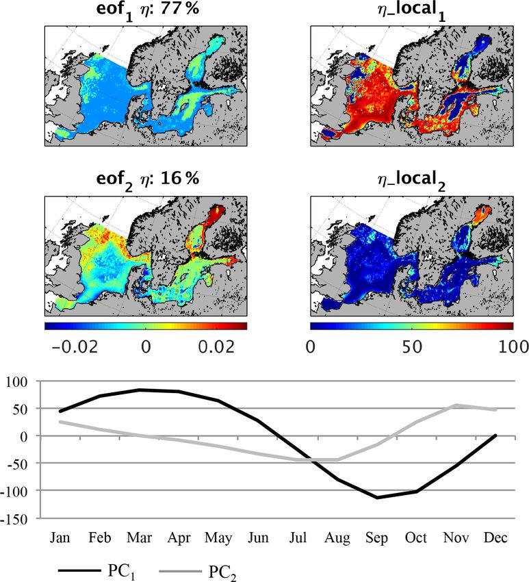
1770                                                                                                    U. Daewel et al.: ECOSMO E2E_v1.0

on food availability. This leads to the following principles               In a second step, fish consumption in each grid box (m, n,
being applied for the fish functional group:                            k) is estimated by weighting the prey-specific components of
                                                                        the consumption in each vertical layer based on the vertical
  1. We neglect horizontal fish migration at spatial scales             distribution of the prey biomass with CX (m, n, k)/PX (m, n)
     larger than one grid cell.                                         such that
  2. The fish group is mobile and, within the given time step           RFiCons (m, n, k) =                                           (9)
     (20 min), able to search the water column for food be-                    2
     yond the vertical extent of a single grid cell. Therefore,
                                                                               X            CZj                     CD
                                                                        PFi         GFi PZj ×          + GFi (PD ) ×
     we assume that the fish group is able to utilise the food                 j =1
                                                                                                 PZj                 PD
     resources available at all depth levels within the water
     column. Consequently, the fish group is not (as other                    + [GFi (PMB )]k = bottom
     variables are) calculated within one sole grid cell, but
     depends on the vertically integrated food resources.               Note that, as fish do not tolerate anoxic conditions, only grid
                                                                        cells featuring positive oxygen concentrations were consid-
  3. The vertical distribution of the fish group and fish pro-
                                                                        ered for the estimate of fish consumption.
     duction depends on the food availability in each grid
                                                                           The loss term for fish includes mortality and excretion.
     cell. This means that during each time step the inte-
     grated fish biomass in the water column is vertically re-          RFiLoss = mFi CFi + εFi CFi                                  (10)
     distributed based on the vertical prey distribution after
     consumption has been estimated.                                    Mortality is considered as a linear mortality rate including
                                                                        biomass losses due to natural mortality and predation. Fish-
   Following these three principles implies that Eq. 1 is sim-          eries mortality was not considered for the standard simula-
plified to ∂C  Fi         ∂CFi
             ∂t + wm (z) ∂z = RFi , where wm (z) is the verti-          tion, but was explicitly addressed in additional scenario ex-
cal migration speed, which is given implicitly by the vertical          periments as described in Sect. 2.4. Excretion is considered
distribution of the fish biomass and is dependent on the ver-           to be related to fish metabolism and consequently to respira-
tical prey distribution. In each grid cell the biological inter-        tion (see the equation for oxygen in Table 4) and hence has
action term (RFi ) is estimated and contains fish consumption           been parameterised as dependent on temperature (Clarke and
(RFiCons ), assimilation efficiency γFi , and a loss term (RFiLoss ):   Johnston, 1999; Gillooly et al., 2001). Reaction kinetics vary
                                                                        with temperature according to the Boltzmann factor k, and
RFi = γFi RFiCons − RFiLoss                                      (7)    we formulated the fish excretion as follows:

                                                                                          θFi
Following principle 2 and 3, RFi is estimated via a two-step                               k ×T K
                                                                                                                 T − T0
                                                                        εFi = µFi e                     ; TK =                       (11)
process. First, total fish consumption at the horizontal loca-                                                   T × T0
tion (m, n) is estimated based on the vertically integrated val-        , where T is given in K and T0 = 273.15 K. All rates are given
ues for fish and prey biomass:                                          in Table 3.
                                                                           Fish and macrobenthos predation, excretion, and mortal-
                   kX
                    max
                                                                        ity are considered in addition to the pelagic lower-trophic-
RFiprod (m, n) =          (RFiCons (m, n, k) × 1zk )             (8)
                   k=1
                                                                        level biological reaction terms (see Daewel and Schrum,
                   X                                                    2013) for nutrients, phytoplankton, zooplankton, detritus,
               =    (GFi (PX ) × PFi ),                                 dissolved organic matter, or sediment (Table 4). While fe-
                    X
                                                                        cal matter is accounted for through the use of assimilation
where PX (X is one of four prey types – herbivorous zoo-                efficiency, the excretion term from both fish and MB di-
plankton Z1 , omnivorous zooplankton Z2 , detritus D, and               rectly contributes to the nutrient reaction terms (see equa-
macrobenthos MB – available for fish in the model) is de-               tion for phosphate and ammonia in Table 4). The new zoo-
fined as the integrated biomass of the prey type X (PX =                plankton mortality term consists of fish predation and ad-
kP
 max                                                                    ditional background mortality, which is 80 % of the back-
     (CXk × 1zk )) over all vertical levels (k = 1 : kmax ) at          ground mortality term used in ECOSMO II. In situ and lab-
k=1
the respective horizontal location (m, n). PFi is the cor-              oratory studies indicate that predation mortality accounts for
responding vertically integrated biomass of fish. Grazing               67 %–75 % of the total mortality (Hirst and Kiørboe, 2002).
rates GFi are estimated using the Michaelis–Menten equation             Other sources of mortality are parasitism, disease, and star-
                   a   PFi                                              vation. However, including fish and macrobenthos as preda-
GFi (PX ) = σFi,X Fi,X
                                    P
                     r+F   with F = aFi,X PX , and aFi,X is
                                            X                           tors in the model does not account for the overall predation
the feeding preference of fish on prey type X (values in Ta-            exerted on zooplankton. By analysing the pelagic food web
ble 2), in a similar manner as for the zooplankton and MB               of the North Sea, Heath (2005) identified the fish consump-
groups.                                                                 tion of omnivorous zooplankton to be 6.7 g C m−2 year−1 on

Geosci. Model Dev., 12, 1765–1789, 2019                                                        www.geosci-model-dev.net/12/1765/2019/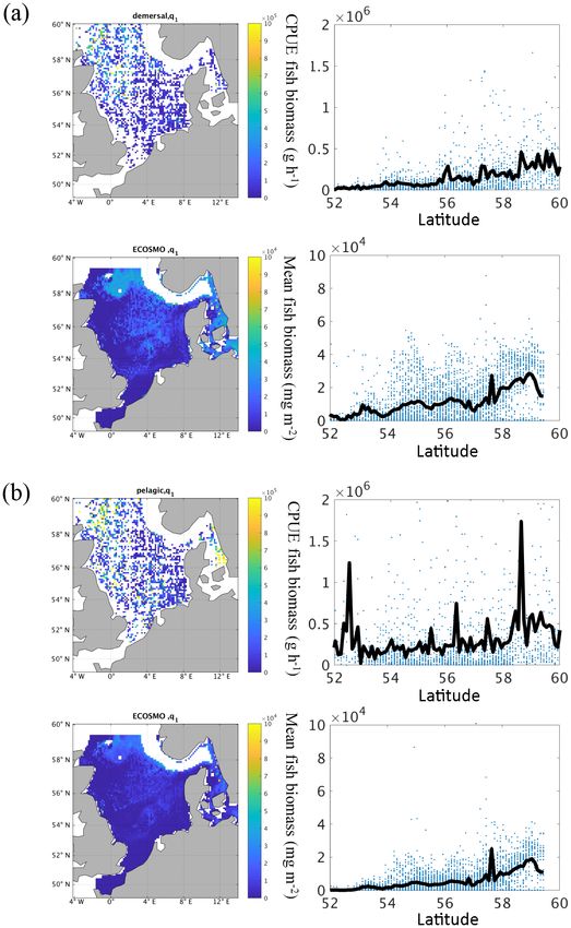
U. Daewel et al.: ECOSMO E2E_v1.0                                                                                                1771

Table 3. Parameters used for the fish functional group.

                       Abbreviation    Definition                                              Value    Units
                       rFi             Fish half-saturation constant                              0.7   mmol C m−3
                       rFi,MB          Fish half-saturation constant (MB prey)                    0.9   mmol C m−3
                       mFi             Fish mortality rate                                     0.001    d−1
                       µFi             Fish excretion rate                                     0.002    d−1
                       θFi             T control parameter excretion                              0.5
                       γFi             Assimilation efficiency                                    0.7
                       σFi,X           Grazing rates F on MB, Z1,2                               0.01   d−1
                       σFi,D           Grazing rates F on D                                    0.005    d−1
                       k               Boltzmann factor                             8.6173324 × 10⁻⁵    eV K−1

Table 4. Changes in the biogeochemical reaction terms (R) of ECOSMO due to the macrobenthos (MB) and fish functional groups.

           State variable              Reaction term
                                                      h             i
           Phytoplankton               RP1,2 = RP1,2 − CMB GMB CP1,2
                                                                                n = bottom
                                                                  CZ
                                               = RZ1,2 − GFi PZ1,2 × P 1,2 − CMB GMB (CX ) /1z n = bottom

           Zooplankton                 RZ1,2
                                                                         Z1,2

           Detritus                    RD = RD − PFi GFi (PD ) × CD
                                                                 PD − [CMB GMB    (CD )]n = bottom

                                              +0.6 (1 − γFi ) RFiCons + mFi CFi

           Dissolved organic matter    RDOM = RDOM − CMB GMB (CDOM ) n = bottom + 0.4 × (1 − γFi ) RFiCons + mFi CFi

                                                + (1 − γMB ) RMBCons + mMB CMB

           Sediments                   RSed. 1 = RSed. 1 − CMB GMB (CSed. 1 ) + 0.6 × (1 − γMB ) RMBCons + mMB CMB

           Phosphate/ammonia           RPO4 /NH4 = RPO4 /NH4 + εFi CFi + MB CMB /1z n = bottom

           Oxygen                      RO2 = RO2 − cC:O2 εFi CFi + MB CMB /1z n = bottom ,
                                       cC:O2 : conversion factor

average. This value was recalculated in Heath (2007), af-               parameter, we performed scenario experiments described in
ter the role of fish pre-recruits feeding on zooplankton was            Sect. 2.4. The degradation products from MB, fish mortality,
more specifically considered, and was reported to amount                and food consumption contribute to particulate organic mat-
to ∼ 7.6 g C m−2 year−1 , whereas the average consumption               ter (POM) and dissolved organic matter (DOM), and it is dis-
by carnivorous zooplankton (euphausids and macroplankton)               tributed between the two partitions POM and DOM with a ra-
was considerably higher at 11 g C m−2 year−1 . As the zoo-              tio 60 % / 40 % (for an explanation see Daewel and Schrum,
plankton groups in the model are not stage resolving, intra-            2013b). As MB species live at the sea floor we assume that
guild predation is not explicitly prescribed as a mortality             the POM generated directly contributes to the sediment pool
term, but is implicitly included in the background mortal-              (Sed. 1), which might contribute to the suspended particulate
ity. Although our model results also suggest that a substan-            matter (D) via resuspension depending on bottom stress. The
tial amount of zooplankton is consumed by macrobenthos in               fish contribution to the POM is added to the detritus pool.
the shallow regions of the North Sea, assuming that about
20 %–30 % of zooplankton mortality stems from the com-                  2.2      Experimental set-up
bined fish and benthos group seems to be a good first guess.
The fact that the reduction of the background mortality rate            To evaluate the model performance after including two new
to 80 % of its initial value does not necessary imply that the          functional groups, we chose to analyse model results from
background mortality is 80 % of the total mortality should be           a 10-year-long simulation period (1980–1989) based on two
taken into consideration. By including a spatially and tempo-           key requirements. First, as the characteristic timescale of the
rally variable mortality term in the model, this term can lo-           Baltic Sea is in the range of 3 decades, and the model results
cally play a much larger (or smaller) role for the overall mor-         also indicate an adaptation period of about 20–30 years for
tality. To evaluate the model sensitivity to the choice of this         fish and MB in the Baltic Sea (not shown), the simulation

www.geosci-model-dev.net/12/1765/2019/                                                       Geosci. Model Dev., 12, 1765–1789, 2019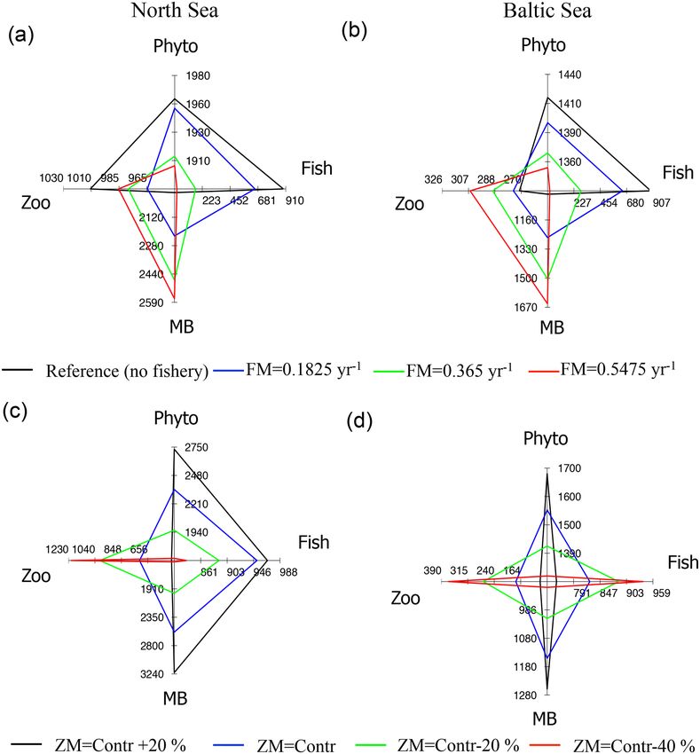
1772 U. Daewel et al.: ECOSMO E2E_v1.0
was started in 1948 to allow for a sufficiently long spin-up onto a 1 m vertical grid to allow for the best local comparison
period with a realistic forcing. Second, we wanted to analyse to the observations, whereas the observations where consid-
a relatively undisturbed period with respect to hydrodynamic ered at the actual sampling depth. The statistical measures
and biogeochemical conditions. Therefore, we chose a period chosen for model analysis were the Pearson correlation co-
prior to the observed regime shift at the end of the 1980s and efficient, the standard deviation and the root mean square
the major Baltic inflow in 1993. deviation presented in a Taylor diagram (Taylor, 2001), and
The model set-up is similar to that described by Daewel the empirical orthogonal functions (EOFs) as described in
and Schrum (2013) for long-term simulations using a hy- von Storch and Zwiers (1999). The EOF analysis is a sta-
drodynamic core model based on HAMSOM (Hamburg tistical method used to understand the major modes of vari-
Shelf Ocean Model), as described in Schrum and Back- ability in multidimensional data fields. A detailed description
haus (1999), with additional modification of the advection on how this method has been applied is given in Daewel et
scheme (Barthel et al., 2012). The model is formulated on al. (2015): “The annual values of the spatially explicit PLS
a staggered Arakawa-C grid with a horizontal resolution of field form an N × M matrix χ (N: number of years; M:
60 × 100 (∼ 10 km) and a 20 min time step. The vertical di- number of wet grid points). The empirical modes are given
mension was resolved with 20 vertical levels; within these by the K eigenvectors of the covariance matrix with non-
levels, the upper 40 m has a layer thickness of 5 m, and the zero eigenvalues. Those modes are temporally constant and
resolution becomes coarser below this point. The model re- have the spatially variable pattern pk (m = 1, . . ., M) where
quires boundary conditions at the atmosphere–ocean bound- k = 1, . . ., K. The time evolution Ak (t = 1, . . ., N ) of each
ary (NCEP/NCAR reanalysis; Kalnay et al., 1996) and at the mode can then be obtained by projecting pk (m) onto the
open boundaries to the North Atlantic. Transport of freshwa- K
P
original data field χ such that: χ (t, m) = pk (m)Ak (t). In
ter and nutrient loads from land is considered. Details on the k=1
boundary and forcing data utilised are given by Daewel and the following sections we will refer to Ak (t) as the principal
Schrum (2013), who also provided a detailed description of components (PCs) and to pk (m) as the EOF. The percentage
analysis methods and validation datasets. of the variance of the field χ explained by mode k is deter-
mined by the respective eigenvalues and is referred to as the
2.3 Datasets and statistical methods for model analysis global explained variance ηg (k). Before using the method to
analyse the spatio-temporal dynamics of the field, the data
As described in Daewel and Schrum (2013), we used ob- were demeaned (to account for the variability only) and nor-
servational data on surface (depth < 10 m) nutrients (nitrate malised (to allow an analysis of the variability independent
and phosphate) in the North Sea, which are made available of its amplitude). The identified modes are not necessarily
by the ICES (International Council for the Exploration of equally significant in all grid points of the data field. Thus,
the Seas, http://www.ices.dk/Pages/default.aspx, last access: the local explained variance ηlocal,k (m) could provide addi-
30 November 2011), for nutrient validation. Observations tional information about the regional relevance of an EOF
and modelled surface nutrients were averaged over the up- mode and the corresponding PC in percent:
per 10 m of the water column and co-located in space and " #
Var χ (m, t) − p k (m)Ak (t)
in time, and corresponding statistics were calculated for the k
ηlocal (m) = 1 − ×100, (12)
sub-areas specified in Fig. 1. The seasonal cycle was not Var (χ (m, t))
removed prior to the analysis. The reason for this was the
N
sparse data situation, which did not allow for the estima- P 2
where Var(X) = X − X(t) denotes the variance of the
tion of a reliable seasonal cycle at each location, in addi- t=1
tion to the seasonal cycle changes from year to year. Thus, field X(t).” In Daewel et al. (2015), the method was applied
removing an average seasonal cycle from the data would to the potential larval survival (PLS) of Atlantic cod (Gadus
add a bias to the data and subsequently increase the level morhua), while in this study it is used on estimated MB and
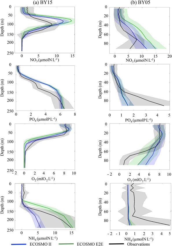
of uncertainty. In the Baltic Sea, we used vertical nutrient fish biomass.
profiles (NO3 , PO4 , and O2 ) at two distinct locations in Information on the North Sea fish community were col-
the Baltic proper: BY05 (lat/long: (∼ 55.1◦ N/15.59◦ E) and lected during the North Sea international Bottom Trawl Sur-
BY15 (lat/long: ∼ 57.2◦ N/20.03◦ E) (see Fig. 1); these loca- vey (NS-IBTS) (ICES, 2012) and are freely available at the
tion were from the Baltic Sea monitoring network (see e.g. International Council for the Exploration of the Sea (http:
http://www.helcom.fi/, last access: 29 April 2019) and have //www.ices.dk/Pages/default.aspx, last access: May 2012).
been continuously sampled since 1970. The data are avail- The NS-IBTS dataset contains spatially resolved, species-
able for download at http://www.ices.dk (last access: Novem- specific information on fish length (for some target species
ber 2016). To account for inconsistencies in sampling fre- also age) and catch per unit effort (CPUE: in numbers cap-
quencies, we co-located model data and observations prior to tured per hour). Given that our model estimated state vari-
estimating average vertical profiles and standard deviations. ables on the base of carbon biomass, we converted fish
For this purpose, the model values were linearly interpolated length and abundance data to fish biomass (in grams cap-
Geosci. Model Dev., 12, 1765–1789, 2019 www.geosci-model-dev.net/12/1765/2019/
U. Daewel et al.: ECOSMO E2E_v1.0 1773
tured per hour) based on published length–weight relation- web parameterisations. We study the structuring effects of
ships (LWRs) for each species sampled in the NS-IBTS be- the new model closure term (higher trophic levels/fisheries)
tween 1980 and 1989 (inclusive of these years). and the effects of changes in background zooplankton
LWRs were derived from Coull et al. (1989), Froese et mortality. The first set of scenario experiments addresses
al. (2014), and FishBase (Froese and Pauly, 2000) for teleost the carbon loss through apex predators and fisheries by
species; McCully et al. (2012) and Templeman (1987) for adding another source of mortality in addition to the nat-
rays and skates; Klaoudatos et al. (2013) for crabs; and Pierce ural fish mortality term. Following the fisheries overview
et al. (1994) and Guerra and Rocha (1994) for squids. Total of the North Sea and Baltic Sea regions as published by
body weight (W ) is a function of total length (L) following ICES (2018a, b), biomass losses due to fisheries are in
the relationship W = aLb , where b is a parameter indicat- the range of 20 %–50 % of the total fish biomass per year
ing isometric growth in body proportions if b ∼ 3, and a is a in both regions. Therefore, for convenience we decided to
parameter describing body shape and condition if b ∼ 3. calculate the fisheries mortality rate by scaling the natural
Calculations were made at the species level, where species mortality rate (= 0.001 d−1 = 0.365 years−1 ) by 0.5, 1, and
names were available, with the a and b parameter estimates 2. As such, three different scenarios were calculated with
taken from published sources in the following order: an average (0.1825 years−1 ), high (0.365 years−1 ), and ex-
treme (0.5475 years−1 ) loss rate. Note that the latter two loss
1. Studies specific to the North Sea (i.e. Coull et al., 1989; rates were chosen to provoke extreme responses in the fish
Froese and Pauly, 2000). biomass, and do not represent realistic catch rates in the ar-
2. If information was not available in the abovemen- eas.
tioned research, studies specific to the British Isles were The second set of experimental scenarios was designed to
utilised (i.e. Coull et al., 1989; Froese and Pauly, 2000; understand the ecosystem response to changes in the zoo-
McCully et al., 2012). plankton natural mortality. This term previously formed the
sole closure term of the system, and the rate has been re-
3. If information was not available in the abovementioned duced by 20 % to account for the additional mortality in-
research, studies specific to the North Atlantic (i.e. duced to the system by MB and fish predation. Here, we
Coull et al., 1989; Froese and Pauly, 2000; McCully et chose four scenarios for the experiment: (1) the control run,
al., 2012; Templeman, 1987). which considered the unchanged zooplankton mortality rate
from ECOSMO II; (2) control −20 %, which is the reference
4. If information was not available in the abovementioned set-up for ECOSMO E2E; (3) control −40 %; and (4) control
research, posterior mean estimates of a and b from a +20 %; scenarios (3) and (4) were used for comparison.
Bayesian hierarchical analysis for the species across all
credible LWR studies were utilised, regardless of loca-
tion (see Froese et al., 2014; Froese and Pauly, 2000).
3 Results and discussion
For some species, e.g. herring, sprat, and mackerel, Coull
et al. (1989) provided mean parameter estimates for each In the following, we discuss the basic characteristics of the
month, or at least some months throughout the year, in ad- model and assess its performance based on 10-year averages
dition to annual estimates. In these cases, we used annual of the model variables. Specifically, we (i) present and dis-
estimates only. If information was only available for genus, cuss the spatial dynamics of the newly introduced functional
family, or order, the a and b parameter estimates for all groups, (ii) discuss the seasonality of the ecosystem compo-
species within that genus, family, or order captured during nents and introduce the MB and fish diet composition emerg-
the surveys were averaged to give a genus-, family-, or order- ing from the model, (iii) present the comparison of the sim-
specific value. If no information was available at any species ulated fish biomass distribution to observed data and repeat
level within a genus, family, or order, the geometric mean the nutrient validation analysis as previously presented for
of that genus, family, or order was computed from the data ECOSMO II in Daewel and Schrum (2013), and (iv) dis-
file accompanying Froese et al. (2014). The data were sorted cuss the model sensitivity with respect to ecosystem model
onto the horizontal model grid based on their sampling lo- closure.
cation. For the data–model comparison we only considered
data from the first quarter of the year, as this was the only 3.1 Description of modelled spatial pattern
systematically surveyed quarter in the considered time pe-
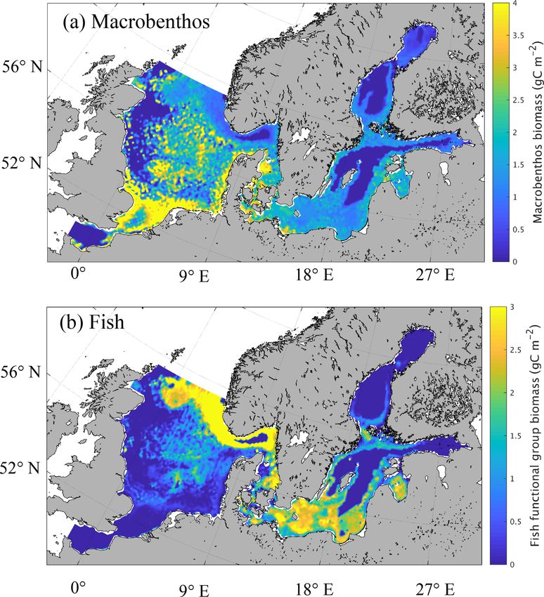
riod (1980–1989) in the survey. The mean spatial patterns of calculated MB and fish verti-
cally integrated biomass for the period from 1980 to 1989
2.4 Scenario definition are presented in Fig. 3. On average, estimated MB biomass
(Fig. 3a) in the North Sea is 1.98 g C m−2 for the time pe-
Two sets of scenarios were performed to evaluate the sim- riod considered. As we will see later, this value is highly
ulated food web response to specific changes in the food sensitive to the parameterisation of zooplankton mortality
www.geosci-model-dev.net/12/1765/2019/ Geosci. Model Dev., 12, 1765–1789, 2019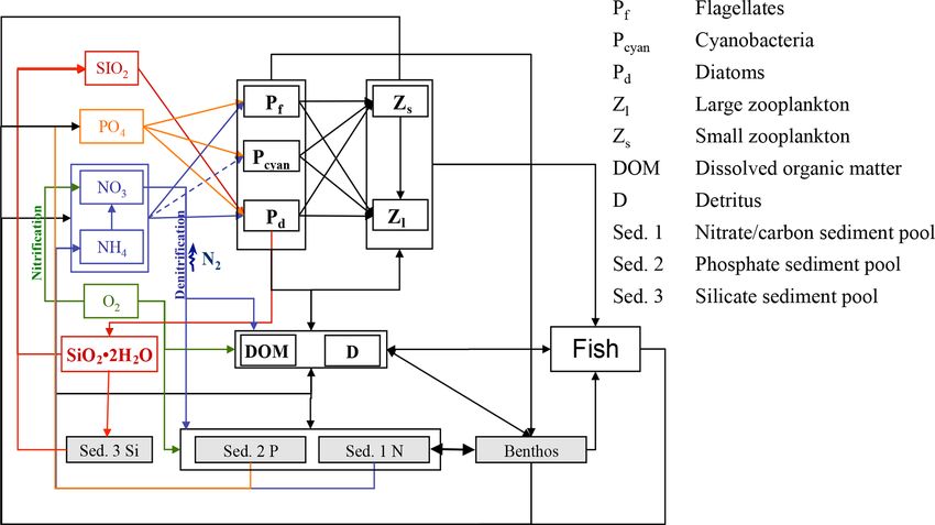
1774                                                                                       U. Daewel et al.: ECOSMO E2E_v1.0

                                                                     100 g WWt m−2 (approx. 0.25–5 g C m−2 ) were reported; it
                                                                     is also within the range of values published by Tomczak et
                                                                     al. (2012), who estimated macrobenthos biomass of about
                                                                     30 t km−2 (which equals 1.5 g C m−2 using an Ecopath with
                                                                     Ecosim Baltic Proper food web model). Furthermore, the
                                                                     spatial distribution of MB modelled using our simplified
                                                                     model is consistent with the spatial distribution of major
                                                                     MB species in the Baltic Sea as presented by Gogina and
                                                                     Zettler (2010) based on species-specific model estimates
                                                                     and observations. This applies specifically to the high abun-
                                                                     dances in the southern Baltic Sea, the near coastal areas, and
                                                                     the Gulf of Riga.
                                                                        Our model estimates the highest MB biomass in both
                                                                     the North Sea and the Baltic Sea in shallower areas, espe-
                                                                     cially near the coast and in bank regions, such as Dogger
                                                                     Bank, Fisher Banks, and Oyster Ground, with a maximum
                                                                     of around 5 g C m−2 found in the southern North Sea. MB
                                                                     production in the model is constrained by the availability of
                                                                     oxygen; therefore, large areas of the central Baltic Sea are not
                                                                     inhabited by macrobenthos. In the North Sea, minimum MB
                                                                     biomass is estimated slightly offshore of the British coast and
                                                                     in the deeper parts of the Norwegian Trench region. These
                                                                     minima in the North Sea were not caused by anoxic condi-
Figure 3. Simulated spatial pattern of annual mean biomass of mac-
                                                                     tions, but by a lack of prey in the respective areas. In contrast,
robenthos (a) and fish (b) (g C m−2 ).
                                                                     the transition zone between the North Sea and the Baltic Sea,
                                                                     including the Skagerrak, Kattegat, the Danish straits, and the
                                                                     Fehmarn Belt, generally exhibits high MB biomass values.
and fisheries effort (cf. Sect. 3.4 and Fig. 12). Heip et               Simulated spatial variability in vertically integrated fish
al. (1992) proposed an average of 7 g ash-free dry weight            biomass shows a structured pattern in both the North Sea and
(AFDW) m−2 based on a synoptic sampling of North Sea                 the Baltic Sea. In the Baltic Sea, maxima of fish biomass are
benthos in April–May 1986. This equates to approximately             simulated in the coastal areas, the Gulf of Riga, in the south-
3.5 g C m−2 when assuming a carbon fraction of the ash-free          ern Baltic Sea (including Arkona Basin, Bornholm Basin,
dry weight of 0.5 (Ingrid Krönke, Senckenberg am Meer,               and Bay of Gdansk), and in the Åland Sea at the entrance
Wilhelmshaven, Germany, personal communication, 2016),               to the Bothnian Sea. The deeper parts of the Eastern Gotland
which is somewhat higher than our model estimates, but               Basin, the Gulf of Finland, and the Gulf of Bothnia, in con-
also includes benthic carnivore biomass (Greenstreet, 1997).         trast, feature very low fish biomass due to low prey biomass
Greenstreet (1997) estimated the biomass of the benthic              and oxygen depletion near the bottom. The modelled spatial
filter-feeder and deposit-feeder guild to be ∼ 3 g C m−2 when        distribution compares well with findings from the nutrient-
the same carbon fraction of 0.5 was applied. Note that the           to-fish model from Radtke et al. (2013). They integrated the
comparison can only be an approximation due to the high              model over a 4-year period from 1980 to 1983. In their model
variability in carbon content among species (e.g. Timmer-            approach, fish follows specific rules for horizontal migration
mann et al., 2012). Observational estimates of North Sea MB          (food availability and spawning). However, their simulated
biomass indicate a decrease in biomass with increasing lati-         spatial distribution of the combined biomass for the three
tude according to Heip et al. (1992), and similar results were       different simulated fish species is very similar to our esti-
obtained from a subsequent sampling project in 2000 (Rees            mates. Differences between the simulated fish distributions
et al., 2007). Particularly high values of MB biomass were           specifically occur in time periods when predefined spawn-
found in the shallow areas of the southern North Sea, includ-        ing areas determine the distribution. Other spatial differences
ing the coastal areas and Dogger Bank (Heip et al., 1992,            were simulated for the Gulf of Finland, where the model by
their Fig. 1), and in the river mouth areas along the English        Radtke et al. (2013) estimated relatively high fish biomass in
coast. This is in clear agreement with what was estimated by         contrast to our model, and around Gotland, where our model
our model.                                                           produces fish biomass maxima potentially fostered by the ad-
    In the Baltic Sea, the MB biomass was modelled to be             ditional availability of macrobenthos as prey, which remains
1.01 g C m−2 on average. This is in the range of what was            unconsidered by Radtke et al. (2013). Interestingly, the dis-
published by Timmermann et al. (2012) based on HEL-                  tribution of fish biomass maxima (estimated by our model)
COM data, where spatially resolved values between 5 and

Geosci. Model Dev., 12, 1765–1789, 2019                                                www.geosci-model-dev.net/12/1765/2019/
U. Daewel et al.: ECOSMO E2E_v1.0 1775
resembles the pattern of cod nursery areas described in the Sparholt (1990) estimated an average fish biomass of about
Baltic Sea by Bagge et al. (1994). 8.6 ×10⁶ t, whereas for the third quarter the average biomass
The structure of modelled North Sea fish biomass is very was estimated to be 13.1 ×10⁶ t. The discrepancy between
distinct with maxima in frontal areas such as the tidal mixing first and third quarter was explained by the migration of the
front in the southern North Sea and around Dogger Bank and western stock of Atlantic mackerel (Scomber scombrus) and
the frontal zone off the German, Danish, and British coast, horse mackerel (Trachurus trachurus) into the North Sea,
and in the Norwegian Trench. Maxima are also modelled in which is not considered by our model. Furthermore, our re-
the Fisher Banks and Oyster Ground as well as the Fladen sults are in agreement with output from an Ecopath with
Ground regions. Minima, in contrast, were estimated in the Ecosim food web model of the North Sea proposed by Mack-
deeper parts of the western North Sea off the British coast, inson and Daskalov (2007), which estimated that the North
the German Bight, and in the English Channel. They partly Sea total fish biomass was ∼ 11 ×106 t in 1991. Indeed, our
resemble the minima estimated for MB, which indicates that modelled estimate is well within the range of previously pub-
fish biomass minima are caused by food shortages in areas lished observations and model results. We suggest that any
with low MB biomass. In particular, off the British Coast, discrepancies are most likely due to our model neglecting
studies from Callaway et al. (2002) and Jennings et al. (1999) fish migration at large scales. When discussing the spatial
indicate high fishing effort, indicating that the model likely variation of estimated fish biomass we need to consider that
underestimates the fish biomass in that region. Potential rea- the model is constrained by the assumption that fish do not
sons for this are the model underestimating zooplankton pro- move horizontally. Thus, we estimate the production poten-
duction in that area (Daewel et al., 2015), and the missing tial for fish in each horizontal grid cell rather than the actual
impact of the open boundary, where neither zooplankton nor fish biomass at a given time and location.
fish were prescribed to enter the model domain.
When integrating fish biomass over the North Sea and 3.2 Seasonal dynamics of ecosystem components and
the Baltic Sea regions, it amounts to ca. 0.462 and diet composition
0.312 ×10⁶ t C respectively. Assuming that the carbon con-
tent of fish is 45 % (Huang et al., 2012; Sterner and George, Values for both MB and fish biomass vary over the course of
2000) and that the AFDW (ash-free dry weight) to wet the year (Fig. 4). While the modelled seasonal amplitude for
weight fish ratio ranges from 0.1 to 0.2, this corresponds fish biomass is relatively small (94.7 mg C m−3 ∼
= 11 % of the
to a simulated total fish biomass in the range of 5.13– mean biomass in the North Sea and 84.8 mg C m−3 ∼ = 9.7 %
10.27 ×10⁶ t for the North Sea and 3.47–6.93 ×10⁶ t for the of the mean biomass in the Baltic Sea) when com-
Baltic Sea. As the AFDW to wet weight ratio is highly vari- pared to the average values, MB seasonality is substantial
able, even within species, depending on factors such as tem- (4.4 g C m−3 ∼= 222 % of the mean biomass in the North Sea
perature, season, and the diet of the fish (Elliott and Hem- and 1.86 g C m−3 ∼ = 183 % of the mean biomass in the Baltic
ingway, 2002), it is difficult to determine an exact value for Sea). Minimum MB and fish biomass is estimated for winter
the simulated entire fish assemblage biomass. The modelled and early spring, and the seasonal maximum is modelled for
estimates of fish biomass are well within the range of what late summer and autumn. The MB maximum lags behind the
has been estimated for total fish biomass based on observa- zooplankton maximum by about 3 months. In contrast to zoo-
tions for the Baltic Sea (Thurow, 1997). Using yield data plankton, the MB minimum does not reach values close to
and age composition data in catches, Thurow (1997) esti- zero; however, the model also simulates a significant stand-
mated total fish biomass in the Baltic Sea for the time pe- ing stock for MB during winter.
riod from 1900 to 1985. His results indicate relatively low In Fig. 4 the seasonal cycles for the phytoplankton and
fish biomass (< 2 ×10⁶ t) for the first half of the century, zooplankton estimates of the ECOSMO E2E run are pre-
but a drastic increase thereafter. For the time period con- sented along with those of the ECOSMO II simulation
sidered here (i.e. 1980–1989) he proposed the fish biomass (Daewel and Schrum, 2013). The seasonal cycles for both
to be around 7 ×10⁶ t. Following ICES (2018b, a), fisheries phytoplankton and zooplankton are clearly affected by the
during the 1980s were in the range of 0.7–1 ×10⁶ t in the consideration of MB and fish. Although the general phyto-
Baltic Sea and 2–3 ×10⁶ t in North Sea. Despite the fact that plankton biomass seasonality and the phenology remain rel-
the model underestimates fish production due to the assump- atively unchanged, the magnitude of the seasonal maximum,
tion that there is no horizontal migration and that no fish mi- especially of the diatom bloom, is significantly increased in
grate over the lateral boundaries, the model’s estimates of spring and early summer in both the North Sea and Baltic
fish biomass in the North Sea would support the landing data Sea regions when the MB and fish groups are included. The
from fisheries during that time period. consideration of seasonally variable MB and fish predation
Estimates for North Sea total biomass for the 1983-1985 on zooplankton imposes a different seasonality on zooplank-
period based on the ICES International Young Fish Sur- ton mortality compared with the constant mortality rate used
vey (IYFS) and the English Groundfish Survey (EGFS) in ECOSMO II (Daewel and Schrum, 2013) and therefore
were published by Sparholt (1990). For the first quarter, impacts zooplankton phenology. The reduced zooplankton
www.geosci-model-dev.net/12/1765/2019/ Geosci. Model Dev., 12, 1765–1789, 20191776 U. Daewel et al.: ECOSMO E2E_v1.0 Figure 4. Average seasonality of ecosystem components. Monthly means averaged for 1980–1989. Solid lines represent ECOSMO E2E, and dashed lines represent ECOSMO II (phytoplankton and zooplankton). Figure 5. Prey composition of (a) macrobenthos (MB) and (b) fish in the North Sea (left) and the Baltic Sea (right). MB feeds on Sed. 1 (or- ganic material in the sediment), DOM / D (dead organic material in the water column; dissolved organic matter / detritus), Z (zooplankton), and P (phytoplankton). Fish feed on Zs (“small” herbivorous zooplankton), Zl (“large” omnivorous zooplankton), D (detritus), and MB. biomass at the beginning of the season due to MB and fish is organic sediments followed by dead organic material, al- predation (Fig. 5) consequently leads to a reduction in phyto- though the percentage of the latter is considerably higher in plankton mortality and an increase in phytoplankton biomass the North Sea than in the Baltic Sea, presumably due to the (top-down process). Additionally, MB competes with zoo- fact that a higher percentage of detritus is resuspended in the plankton for resources and thereby changes zooplankton sea- tidally influenced, highly turbulent areas of the North Sea. sonality, especially in autumn in the North Sea when MB Zooplankton and phytoplankton are included in the MB diet biomass is highest and it preys dominantly on dead organic when available in spring and summer. The fish prey compo- material and phytoplankton (Fig. 5). sition (Fig. 5b) is very similar in both sub-areas: MB domi- An overview of the seasonal feeding dynamics can be ob- nates the diet in the autumn and winter months and omnivo- tained by identifying the monthly prey composition for MB rous (large) zooplankton dominates in summer. Detritus con- (Fig. 5a) and fish (Fig. 5b) in the North Sea and the Baltic tributes a significant food source in March and April, while Sea. For MB, the major food source throughout the year small zooplankton only appears in autumn and in very low Geosci. Model Dev., 12, 1765–1789, 2019 www.geosci-model-dev.net/12/1765/2019/
You can also read