Regional variation in the effectiveness of methane-based and land-based climate mitigation options
←
→
Page content transcription
If your browser does not render page correctly, please read the page content below
Earth Syst. Dynam., 12, 513–544, 2021
https://doi.org/10.5194/esd-12-513-2021
© Author(s) 2021. This work is distributed under
the Creative Commons Attribution 4.0 License.

       Regional variation in the effectiveness of methane-based
             and land-based climate mitigation options
         Garry D. Hayman1 , Edward Comyn-Platt1 , Chris Huntingford1 , Anna B. Harper2 , Tom Powell3 ,
              Peter M. Cox2 , William Collins4 , Christopher Webber4 , Jason Lowe5,6 , Stephen Sitch3 ,
      Joanna I. House7 , Jonathan C. Doelman8 , Detlef P. van Vuuren8,9 , Sarah E. Chadburn2 , Eleanor Burke6 ,
                                                and Nicola Gedney10
                            1 UK  Centre for Ecology & Hydrology, Wallingford, OX10 8BB, UK
         2 Collegeof Engineering, Mathematics, and Physical Sciences, University of Exeter, Exeter, EX4 4QF, UK
                3 College of Life and Environmental Sciences, University of Exeter, Exeter, EX4 4QF, UK
                       4 Department of Meteorology, University of Reading, Reading, RG6 6BB, UK
                        5 School of Earth and Environment, University of Leeds, Leeds, LS2 9JT, UK
                               6 Met Office Hadley Centre, FitzRoy Road, Exeter, EX1 3PB, UK
                     7 Cabot Institute for the Environment, University of Bristol, Bristol, BS8 1SS, UK
            8 Department of Climate, Air and Energy, Netherlands Environmental Assessment Agency (PBL),

                                    P.O. Box 30314, 2500 GH The Hague, the Netherlands
                            9 Copernicus Institute of Sustainable Development, Utrecht University,

                                      Heidelberglaan 2, 3584 CS Utrecht, the Netherlands
        10 Met Office Hadley Centre, Joint Centre for Hydrometeorological Research, Wallingford, OX10 8BB, UK

                                   Correspondence: Garry D. Hayman (garr@ceh.ac.uk)

                                    Received: 28 April 2020 – Discussion started: 17 June 2020
                          Revised: 23 February 2021 – Accepted: 5 March 2021 – Published: 5 May 2021

      Abstract. Scenarios avoiding global warming greater than 1.5 or 2 ◦ C, as stipulated in the Paris Agreement, may
      require the combined mitigation of anthropogenic greenhouse gas emissions alongside enhancing negative emis-
      sions through approaches such as afforestation–reforestation (AR) and biomass energy with carbon capture and
      storage (BECCS). We use the JULES land surface model coupled to an inverted form of the IMOGEN climate
      emulator to investigate mitigation scenarios that achieve the 1.5 or 2 ◦ C warming targets of the Paris Agreement.
      Specifically, within this IMOGEN-JULES framework, we focus on and characterise the global and regional
      effectiveness of land-based (BECCS and/or AR) and anthropogenic methane (CH4 ) emission mitigation, sepa-
      rately and in combination, on the anthropogenic fossil fuel carbon dioxide (CO2 ) emission budgets (AFFEBs)
      to 2100. We use consistent data and socio-economic assumptions from the IMAGE integrated assessment model
      for the second Shared Socioeconomic Pathway (SSP2). The analysis includes the effects of the methane and
      carbon–climate feedbacks from wetlands and permafrost thaw, which we have shown previously to be signifi-
      cant constraints on the AFFEBs.
         Globally, mitigation of anthropogenic CH4 emissions has large impacts on the anthropogenic fossil fuel emis-
      sion budgets, potentially offsetting (i.e. allowing extra) carbon dioxide emissions of 188–212 Gt C. This is be-
      cause of (a) the reduction in the direct and indirect radiative forcing of methane in response to the lower emissions
      and hence atmospheric concentration of methane and (b) carbon-cycle changes leading to increased uptake by
      the land and ocean by CO2 -based fertilisation. Methane mitigation is beneficial everywhere, particularly for the
      major CH4 -emitting regions of India, the USA, and China. Land-based mitigation has the potential to offset 51–
      100 Gt C globally, the large range reflecting assumptions and uncertainties associated with BECCS. The ranges
      for CH4 reduction and BECCS implementation are valid for both the 1.5 and 2 ◦ C warming targets. That is the
      mitigation potential of the CH4 and of the land-based scenarios is similar for regardless of which of the final

Published by Copernicus Publications on behalf of the European Geosciences Union.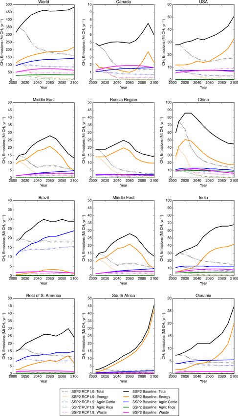
514              G. D. Hayman et al.: Regional variation in the effectiveness of methane-based climate mitigation options

       stabilised warming levels society aims for. Further, both the effectiveness and the preferred land management
       strategy (i.e. AR or BECCS) have strong regional dependencies. Additional analysis shows extensive BECCS
       could adversely affect water security for several regions. Although the primary requirement remains mitigation
       of fossil fuel emissions, our results highlight the potential for the mitigation of CH4 emissions to make the Paris
       climate targets more achievable.

1   Introduction                                                   lished estimates are similar for the two warming targets, with
                                                                   between 380–700 Mha required for the 2 ◦ C target (Smith
The stated aims of the Paris Agreement of the United Na-           et al., 2016) and greater than 600 Mha for the 1.5 ◦ C target
tions Framework Convention on Climate Change (UNFCCC,              (van Vuuren et al., 2018). This is because the land require-
2015) are “to hold the increase in global average temper-          ments for bioenergy production differ strongly across the
ature to well below 2 ◦ C and to pursue efforts to limit the       different SSPs, depending on assumptions about the contri-
increase to 1.5 ◦ C”. The global average surface temperature       bution of residues, assumed yields and yield improvements,
for the decade 2006–2015 was 0.87 ◦ C above pre-industrial         start dates of implementation, and the rates of deployment.
levels and is likely to reach 1.5 ◦ C between the years 2030       While the CDR figures assume optimism about the mitiga-
and 2052 if global warming continues at current rates (IPCC,       tion potential of BECCS, concerns have been raised about
2018). The IPCC Special Report on Global Warming of                the potentially detrimental impacts of BECCS on food pro-
1.5 ◦ C (IPCC, 2018) gives the median remaining carbon bud-        duction, water availability and biodiversity (e.g. Heck et al.,
gets between 2018 and 2100 as 770 Gt CO2 (210 Gt C) and            2018; Krause et al., 2017). Others note the risks and query the
1690 Gt CO2 (∼ 461 Gt C) to limit global warming to 1.5 ◦ C        feasibility of large-scale deployment of BECCS (e.g. Ander-
and 2 ◦ C, respectively. These budgets represent ∼ 20 and          son and Peters, 2016; Vaughan and Gough, 2016; Vaughan et
∼ 41 years at present-day emission rates. The actual bud-          al., 2018).
gets could, however, be smaller, as they exclude Earth sys-           Harper et al. (2018) find the overall effectiveness of
tem feedbacks such as CO2 released by permafrost thaw              BECCS to be strongly dependent on the assumptions con-
or CH4 released by wetlands. Meeting the Paris Agree-              cerning yields, the use of initial above-ground biomass that
ment goals will, therefore, require sustained reductions in        is replaced, and the calculated fossil fuel emissions that are
sources of fossil carbon emissions, other long-lived anthro-       offset in the energy system. Notably, if BECCS involves re-
pogenic greenhouse gases (GHGs), and some short-lived cli-         placing ecosystems that have higher carbon contents than en-
mate forcers (SLCFs) such as methane (CH4 ), alongside in-         ergy crops, then AR and avoided deforestation can be more
creasingly extensive implementations of carbon dioxide re-         efficient than BECCS for atmospheric CO2 removal over this
moval (CDR) technologies (IPCC, 2018). Accurate informa-           century (Harper et al., 2018).
tion is needed about the range and efficacy of options avail-         Mitigation of the anthropogenic emissions of non-CO2
able to achieve this.                                              GHGs such as CH4 and of SLCFs such as black carbon have
   Biomass energy with carbon capture and storage (BECCS)          been shown to be attractive strategies with the potential to re-
and afforestation–reforestation (AR) are among the most            duce projected global mean warming by 0.22–0.5 ◦ C by 2050
widely considered CDR technologies in the climate and en-          (Shindell et al., 2012; Stohl et al., 2015). It should be noted
ergy literature (Minx et al., 2018). For scenarios consis-         that these were based on scenarios with continued use of fos-
tent with a 2 ◦ C warming target, the review by Smith et           sil fuels. Through the link to tropospheric ozone (O3 ), there
al. (2016) finds this may require (i) a median removal of          are additional co-benefits of CH4 mitigation for air qual-
3.3 Gt C yr−1 from the atmosphere through BECCS by 2100            ity, plant productivity and food production (Shindell et al.,
and (ii) a mean CDR through AR of 1.1 Gt C yr−1 by 2100,           2012), and carbon sequestration (Oliver et al., 2018). Con-
giving a total CDR equivalent to 47 % of present-day emis-         trol of anthropogenic CH4 emissions leads to rapid decreases
sions from fossil fuel and other industrial sources (Le Quéré      in its atmospheric concentration, with an approximately 9-
et al., 2018). Although there are fewer scenarios that look        year removal lifetime (and as such is an SLCF). Further-
specifically at the 1.5 ◦ C pathway, BECCS is still the major      more, many CH4 mitigation options are inexpensive or even
CDR approach (Rogelj et al., 2018). For the default assump-        cost-negative through the co-benefits achieved (Stohl et al.,
tions in Fuss et al. (2018), BECCS would remove a median           2015), although expenditure becomes substantial at high lev-
of 4 Gt C by 2100 and a total of 41–327 Gt C from the at-          els of mitigation (Gernaat et al., 2015). The extra “allowable”
mosphere during the 21st century, equivalent to about 4–30         carbon emissions from CH4 mitigation can make a substan-
years of current annual emissions. The land requirements for       tial difference to the feasibility or otherwise of achieving the
BECCS will be greater for the 1.5 ◦ C target within a given        Paris climate targets (Collins et al., 2018).
shared socio-economic pathway (e.g. SSP2), although pub-

Earth Syst. Dynam., 12, 513–544, 2021                                                 https://doi.org/10.5194/esd-12-513-2021
G. D. Hayman et al.: Regional variation in the effectiveness of methane-based climate mitigation options                      515

   Some increases in atmospheric CH4 are not related to di-        climatic aNomalies” (Sect. 2.2) (Comyn-Platt et al., 2018a;
rect anthropogenic activity but indirectly to climate change       Huntingford et al., 2010) is an intermediate complexity cli-
triggering natural carbon and methane–climate feedbacks.           mate model, which emulates 34 models in the CMIP5 climate
These effects could act as positive feedbacks and thus in the      model ensemble. Hence, our radiative forcing (RF) trajecto-
opposite direction to the mitigation of anthropogenic CH4          ries have uncertainty bounds, reflecting the different climate
sources. Wetlands are the largest natural source of CH4 to         sensitivities of existing climate models.
the atmosphere and these emissions respond strongly to cli-           For each radiative forcing pathway, we subtract the in-
mate change (Gedney et al., 2019; Melton et al., 2013). A          dividual RF components for non-CO2 and non-CH4 radia-
second natural feedback is from permafrost thaw. In a warm-        tively active gases that are perturbed by human activity, us-
ing climate, the resulting microbial decomposition of previ-       ing baseline and mitigation scenarios taken from the IMAGE
ously frozen organic carbon is potentially one of the largest      integrated assessment model. Following this, for CH4 we
feedbacks from terrestrial ecosystems (Schuur et al., 2015).       represent its atmospheric chemistry by a single atmospheric
As the carbon and CH4 climate feedbacks from natural wet-          lifetime to translate the methane emissions into atmospheric
lands and permafrost thaw could be substantial, this causes        concentrations. The related RF for CH4 is also subtracted
a reduction in anthropogenic CO2 emission budgets compat-          from the overall value. Hence, the remaining RF is that
ible with climate change targets (Comyn-Platt et al., 2018a;       available for changes to atmospheric CO2 concentration. The
Gasser et al., 2018).                                              IMOGEN model uses pattern scaling, again fitted to the same
   This paper models the potential for mitigation of green-        34 climate models, to estimate local changes in near-surface
house gases to contribute to meeting the Paris targets of lim-     meteorology. Combined with our global temperature path-
iting global warming to 1.5 ◦ C and 2 ◦ C, respectively. Specif-   ways, these pattern-based changes (as well as atmospheric
ically, we investigate the effectiveness of mitigation of an-      CO2 concentration) drive the Joint UK Land-Environment
thropogenic methane emissions and land-based mitigation            Simulator land surface model (JULES, Sect. 2.1) (Best et al.,
(e.g. implementation of BECCS and AR), combining results           2011; Clark et al., 2011). JULES estimates atmosphere–land
from three recent papers (Collins et al., 2018; Comyn-Platt        CO2 exchange, and IMOGEN similarly contains a single
et al., 2018a; Harper et al., 2018). We determine the effec-       global description of oceanic CO2 draw-down. These two es-
tiveness of these approaches in terms of their impact on the       timates of carbon exchanges with the land and ocean, respec-
anthropogenic fossil fuel CO2 emissions budget consistent          tively, in conjunction with atmospheric storage being linear
with stabilising temperature at 1.5 and 2 ◦ C of warming. The      in the CO2 pathway, finally determine by simple summa-
more effective the mitigation option, the larger the fossil fuel   tion compatible CO2 emissions from fossil fuel burning. We
CO2 emissions budget can be consistent with stabilisation at       call this the anthropogenic (CO2 ) fossil fuel emission bud-
a given level. We estimate the impact of these mitigation sce-     gets (AFFEB) compatible with the warming pathway, subject
narios relative to an existing scenario of greenhouse gas con-     to the assumptions made for non-CO2 forcings.
centrations (based on the IMAGE SSP2 baseline), spanning              Our numerical simulation structure allows us to investi-
uncertainties in both climate model projections (both global       gate the implications of three different key changes on AF-
warming and regional climate change), process representa-          FEB for stabilisation at both 1.5 and 2.0 ◦ C and in a structure
tion, and the efficacy of BECCS. Section 2 provides a brief        that captures features of a full set of climate models. First
description of the models, the experimental set-up, and the        and maybe most importantly, we work to understand how
key datasets used in the model runs and subsequent analysis.       regional reductions in CH4 emissions allow higher values
Section 3 presents and discusses the results, starting with a      of AFFEB. Second, we consider how alternative scenarios
global perspective before addressing the regional dimension.       of BECCS implementation alter atmosphere–land CO2 ex-
For BECCS, we additionally investigate the sensitivity to key      changes and again present the resultant implications for AF-
assumptions and consider the implications for water security.      FEB. Third, we determine how the newer understanding of
Section 4 contains our conclusions.                                warming impacts on wetland methane emissions also affects
                                                                   AFFEB. Figure 1 captures the modelling framework, deriva-
                                                                   tion of AFFEB, and our numerical experiments in a single
2   Approach and methodology                                       overall schematic diagram.
                                                                      Each of the scenarios investigated using the IMOGEN-
Our overall modelling strategy is as follows. The starting         JULES framework comprises 2 ensembles of 136 members,
point is the prescription of global temperature profiles that      one ensemble for each of the warming targets. We make use
match the historical record, followed by a transition to a fu-     of these ensembles to derive an “uncertainty” in the derived
ture stabilisation at either 1.5 or 2.0 ◦ C above pre-industrial   carbon budgets, specifically from climate change (as given
levels. For these profiles, we then determine the related path-    by the 34 CMIP5 models) and from key land surface pro-
ways in atmospheric radiative forcing by inversion of the          cesses (methane emissions from wetlands and the ozone veg-
global energy balance component of the IMOGEN impacts              etation damage). The climate change uncertainty comprises
model. IMOGEN “Integrated Model Of Global Effects of               both the range of climate sensitivities of the CMIP5 models

https://doi.org/10.5194/esd-12-513-2021                                               Earth Syst. Dynam., 12, 513–544, 2021
516 G. D. Hayman et al.: Regional variation in the effectiveness of methane-based climate mitigation options
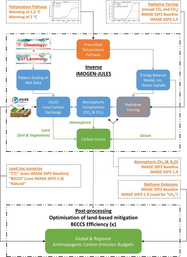
Figure 1. Schematic of the modelling approach and the workflow. The coloured boxes and text show the key components of the inverted
IMOGEN-JULES model (blue), the prescribed and input data used in this study (orange), and the outputs (green).
and the different regional patterns in the models. We use the 1. Land use. We adopt the approach used by Harper et
median of the 136-member ensemble as the central value to al. (2018) and prescribe managed land use and land use
derive the carbon budgets and the interquartile range (25 %– change (LULUC). On land used for agriculture, C3 and
75 %) for the uncertainty. C4 grasses are allowed to grow to represent crops and
pasture. The land use mask consists of an annual frac-
2.1 The JULES model tion of agricultural land in each grid cell. Historical LU-
LUC is based on the HYDE 3.1 dataset (Klein Gold-
We use the JULES land surface model (Best et al., 2011; ewijk et al., 2011), and future LULUC is based on
Clark et al., 2011), release version 4.8 but with a number two scenarios (SSP2 RCP1.9 and SSP2 baseline), which
of additions required specifically for our analysis. were developed for use in the IMAGE integrated assess-
Earth Syst. Dynam., 12, 513–544, 2021 https://doi.org/10.5194/esd-12-513-2021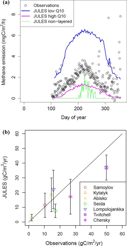
G. D. Hayman et al.: Regional variation in the effectiveness of methane-based climate mitigation options                          517

    ment model (IAM) (Doelman et al., 2018; van Vuuren              in our study (JULES low Q10 –JULES high Q10 ) cap-
    et al., 2017) (see also Sect. 2.3).                             tures the range of uncertainty in the observations. In
                                                                    Fig. 2b, the error bars denote the lower and upper es-
    Natural vegetation is represented by nine plant func-
                                                                    timates from the low and high Q10 simulations. The
    tional types (PFTs): broadleaf deciduous trees, tropi-
                                                                    symbols represent the mean value between these es-
    cal broadleaf evergreen trees, temperate broadleaf ev-
                                                                    timates. Further, the layered methane scheme used in
    ergreen trees, needle-leaf deciduous trees, needle-leaf
                                                                    this work gives a better description of the shoulder sea-
    evergreen trees, C3 and C4 grasses, and deciduous and
                                                                    son emissions when compared with the original, non-
    evergreen shrubs (Harper et al., 2016). These PFTs are
                                                                    layered methane scheme in JULES. The multi-layered
    in competition for space in the non-agricultural fraction
                                                                    scheme allows an insulated sub-surface layer of active
    of grid cells, based on the TRIFFID (Top-down Rep-
                                                                    methanogenesis to continue after the surface has frozen.
    resentation of Interactive Foliage and Flora Including
                                                                    These model developments not only improve the sea-
    Dynamics) dynamic vegetation module within JULES
                                                                    sonality of the emissions but more importantly for this
    (Clark et al., 2011). A further four PFTs are used to rep-
                                                                    study capture the release of carbon as CH4 from deep
    resent agriculture (C3 and C4 crops and C3 and C4 pas-
                                                                    soil layers, including thawed permafrost. Further evalu-
    ture), and harvest is calculated separately for food and
                                                                    ation of the multi-layer scheme can be found in Chad-
    bioenergy crops (see Sect. 2.4.3, where we describe the
                                                                    burn et al. (2020).
    modelling of carbon removed via bioenergy with CCS).
    When natural vegetation is converted to managed agri-        3. Methane from wetlands. Following Comyn-Platt et
    cultural land, the vegetation carbon removed is placed          al. (2018a), we also use the multi-layered soil carbon
    into woody product pools that decay at various rates            scheme described in (2) above to give the local land–
    back into the atmosphere (Jones et al., 2011). Hence,           atmosphere CH4 flux, ECH4 (kg C m−2 s−1 ):
    the carbon flux from LULUC is not lost from the sys-
    tem. There are also four non-vegetated surface types:                                  s pools
                                                                                         nCX                 Xm
                                                                                                            z=3
    urban, water, bare soil, and ice.                               ECH4 = k · fwetl ·               κi ·           e−γ z Csi,z
                                                                                            i=1             z=0 m
 2. Soil carbon. Following Comyn-Platt et al. (2018a),                                   0.1(Tsoilz −T0 )
                                                                          · Q10 Tsoilz                       ,                    (1)
    we also use a 14-layered soil column for both hydro-
    thermal (Chadburn et al., 2015) and carbon dynamics             where k is a dimensionless scaling constant such that the
    (Burke et al., 2017b). Burke et al. (2017a) demonstrated        global annual wetland CH4 emissions are 180 Tg CH4
    that modelling the soil carbon fluxes as a multi-layered        in 2000 (as described in Comyn-Platt et al., 2018a),
    scheme improves estimates of soil carbon stocks and             z is the depth in soil column (in m), i is the soil car-
    net ecosystem exchange. In addition to the vertically           bon pool, fwetl (–) is the fraction of wetland area in the
    discretised respiration and litter input terms, the soil–       grid cell, κi (s−1 ) is the specific respiration rate of each
    carbon balance calculation also includes a diffusivity          pool (Table 8 of Clark et al., 2011), Cs (kg m−2 ) is soil
    term to represent cryoturbation–bioturbation processes.         carbon, and Tsoil (K) is the soil temperature. The decay
    The freeze–thaw process of cryoturbation is particu-            constant γ (= 0.4 m−1 ) describes the reduced contribu-
    larly important in cold permafrost-type soils (Burke et         tion of CH4 emission at deeper soil layers due to inhib-
    al., 2017a). Following Burke et al. (2017b), we diag-           ited transport and increased oxidation through overlay-
    nose permafrost wherever the deepest soil layer is be-          ing soil layers. This representation of inhibition and of
    low 0 ◦ C (assuming that this layer is below the depth of       the pathways for CH4 release to the atmosphere (e.g. by
    zero annual amplitude, i.e. where seasonal changes in           diffusion, ebullition, and vascular transport) is a simpli-
    ground temperature are negligible (≤ 0.1 ◦ C)). Further,        fication. However, previous work that explicitly repre-
    for permafrost regions, there is an additional variable to      sented these processes showed little to no improvement
    trace or diagnose “old” carbon and its release from per-        when compared with in situ observations (McNorton et
    mafrost as it thaws.                                            al., 2016). We do not model CH4 emissions from fresh-
    The multi-layered methanogenesis scheme improves                water lakes (and oceans).
    the representation of high latitude CH4 emissions,              Comyn-Platt et al. (2018a) varied Q10 in Eq. (1) to
    where previous studies underestimated production at             encapsulate a range of methanogenesis process uncer-
    cold permafrost sites during “shoulder seasons” (Zona           tainty. They derive Q10 values for each GCM con-
    et al., 2016). Figure 2 shows the annual cycle in the           figuration to represent two wetland types identified
    observed and modelled wetland CH4 emissions at the              in Turetsky et al. (2014) (“poor-fen” and “rich-fen”).
    Samoylov Island field site (Fig. 2a) and a comparison           They also include a third “low-Q10 ”, which gives in-
    of observed and modelled annual mean fluxes at this             creased importance to high-latitude emissions. Their
    and other sites (Fig. 2b). The range of uncertainty used        ensemble spread was able to describe the magnitude

https://doi.org/10.5194/esd-12-513-2021                                            Earth Syst. Dynam., 12, 513–544, 2021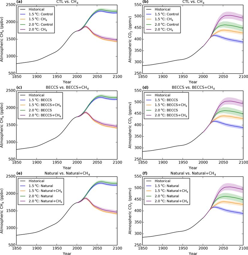
518               G. D. Hayman et al.: Regional variation in the effectiveness of methane-based climate mitigation options

      and distribution of present-day CH4 emissions from
      natural wetlands, according to the models used in the
      then-current global methane assessment (Saunois et al.,
      2016). Here, we use the “low-Q10 ” value of Comyn-
      Platt et al. (2018a) (= 2.0) and adopt a “high-Q10 ”
      value of ∼ 4.8 from the rich-fen parameterisation. The
      two Q10 values used here still capture the full range of
      the methanogenesis process uncertainty.

 4. Ozone vegetation damage. We use a JULES config-
    uration including ozone deposition damage to plant
    stomata, which affects land–atmosphere CO2 exchange
    (Sitch et al., 2007). JULES requires surface atmo-
    spheric ozone concentrations, O3 (ppb), for the dura-
    tion of the simulation period (1850–2100). As in Collins
    et al. (2018), we do not model tropospheric ozone
    production from CH4 explicitly in IMOGEN. Instead,
    we use two sets of monthly near-surface O3 concen-
    tration fields (January–December) from HADGEM3-
    A GA4.0 model runs, with the sets corresponding to
    low (1285 ppbv) and high (2062 ppbv) global mean at-
    mospheric CH4 concentrations (Stohl et al., 2015). We
    assume that the atmospheric O3 concentration in each
    grid cell responds linearly to the atmospheric CH4 con-
    centration. We derive separate linear relationships for
    each month and grid cell and use these to calculate the
    surface O3 concentration from the corresponding global
    atmospheric CH4 concentration as it evolves during the
    IMOGEN run (Sect. 2.2.1). We use CH4 concentration
    profiles from the IMAGE SSP2 Baseline and RCP1.9             Figure 2. (a) Observed (circles) and modelled wetland methane
    scenarios (Sect. 2.3.1) adjusted for natural methane         emissions at the Samoylov Island field site. Modelled wetland
    sources (see 3 above and Sect. 2.3.3). We undertake runs     methane emissions are shown for the standard JULES non-layered
                                                                 soil carbon configuration (green) and for the JULES layered soil
    using both the “high” and “low” vegetation ozone dam-
                                                                 carbon configurations with low (blue line) and high (magenta
    age parameter sets (Sitch et al., 2007).
                                                                 line) Q10 temperature sensitivities; the low Q10 configuration
                                                                 gives higher methane emissions at high-latitude sites such as the
                                                                 Samoylov Island field site. The methane emission data are prelimi-
2.2     The IMOGEN intermediate complexity climate               nary and were provided by Lars Kutzbach and David Holl. (b) Com-
        model                                                    parison of observed and modelled annual mean wetland CH4 emis-
                                                                 sion fluxes at a number of northern high-latitude and temperate
2.2.1    IMOGEN                                                  sites. The error bars denote the lower and upper estimates from
                                                                 the low and high Q10 simulations. The symbols represent the mean
The IMOGEN climate impacts model (Huntingford et al.,
                                                                 value between these estimates.
2010) uses “pattern-scaling” to estimate changes to the seven
meteorological variables required to drive JULES. Hunting-
ford et al. (2010) assume that changes in local temperature,     culated (CO2 and CH4 ) or prescribed (for other atmospheric
precipitation, humidity, wind speed, surface short-wave and      contributors) on a yearly time step.
long-wave radiation, and pressure are linear in global warm-
ing. Spatial patterns of each variable (based on the 34 GCM      1Q(total) = 1Q (CO2 ) + 1Q (non CO2 GHGs)
simulations in CMIP5, Comyn-Platt et al., 2018a) are mul-                   + 1Q(aerosols and other climate forcers)           (2)
tiplied by the amount of global warming over land, 1TL , to
give local monthly predictions of climate change. When us-       The EBM includes a simple representation of the ocean up-
ing IMOGEN in forward mode, 1TL is calculated with an            take of heat and CO2 and uses a separate set of four pa-
energy balance model (EBM) as a function of the overall          rameters for each climate and Earth system model emulated
changes in radiative forcing, 1Q (W m−2 ). 1Q is the sum         (Huntingford et al., 2010): the climate feedback parameters
of the atmospheric greenhouse gas contributions (Eq. 2) (Et-     over land and ocean, λl and λo (W m−2 K−1 ), respectively,
minan et al., 2016), which in the forward mode are either cal-   the oceanic “effective thermal diffusivity”, κ (W m−1 K−1 ),

Earth Syst. Dynam., 12, 513–544, 2021                                               https://doi.org/10.5194/esd-12-513-2021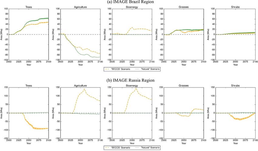
G. D. Hayman et al.: Regional variation in the effectiveness of methane-based climate mitigation options                     519

representing the ocean thermal inertia and a land–sea temper-      emissions is a larger source of uncertainty than that from the
ature contrast parameter, ν, linearly relating warming over        projected climate spread of the 34 GCMs. We quantify this
land, 1Tl (K), to warming over ocean, 1To (K), as 1Tl =            uncertainty in our experimental design by using two values
ν1To . The climate feedback parameters (λl and λo ) are cal-       of Q10 (see Sect. 2.1).
ibrated using model-specific data for the top of the atmo-            In response to our dynamic interactive calculations of at-
sphere radiative fluxes, the mean land and ocean surface tem-      mospheric CH4 concentrations, we derive the related change
peratures, and an estimate of the radiative forcing modelled       in methane radiative forcing (RF). We use the formulation
for the CO2 changes.                                               from Etminan et al. (2016), which accounts for the short-
   The atmospheric CH4 concentrations available from the           wave absorption by CH4 and the overlap with N2 O. The at-
IMAGE database (see Sect. 2.3.1) assume a constant annual          mospheric oxidation of methane (by the hydroxyl radical)
wetland CH4 emission (van Vuuren et al., 2017). However,           leads to the production of tropospheric ozone and strato-
these emissions have interannual variability and a positive        spheric water vapour. We calculate these indirect contribu-
climate feedback (Comyn-Platt et al., 2018a; Gedney et al.,        tions of methane to the overall radiative forcing, follow-
2019), and their correct representation is a central part of our   ing the approach for methane adopted in our previous work
study. We follow the same approach that we used in our pre-        (Collins et al., 2018; Comyn-Platt et al., 2018a; Gedney et
vious studies (Collins et al., 2018; Comyn-Platt et al., 2018a;    al., 2019). Collins et al. (2018) represent the forcing con-
Gedney et al., 2019). As the IMOGEN-JULES modelling                tributions from O3 and stratospheric water vapour as lin-
framework does not have an explicit representation of the at-      ear functions of the CH4 mixing ratio, based on the anal-
mospheric chemistry of methane, we represent the oxidation         ysis presented in IPCC AR5 (Myhre et al., 2013). The
and hence loss of CH4 by a single lifetime (τ ).                   indirect methane forcings amount to 2.36 × 10⁻⁴ ± 1.09 ×
                                                                   10−4 W m−2 per ppb CH4 (i.e. 0.65 ± 0.3 times the CH4 ra-
d ([CH4 ] − [CH4 ]IMAGE )    nX
                                                                   diative efficiency). Hence, we incorporate the indirect effects
                          =C      F [CH4 ]
            dt                                                     of these CH4 emission changes by an approximation, multi-
                            X               o
                          −   F [CH4 ]IMAGE                        plying the CH4 radiative forcing by 1.65.
                                                                      In this study, we use the inverse version of IMOGEN,
                                 [CH4 ] − [CH4 ]REF                which follows prescribed temperature pathways (Fig. 3a), to
                             −                              (3)
                                         τ                         derive the total radiative forcing (1Q[total]) and then the
Here, [CH4 ] and [CH4 ]IMAGE are the atmospheric methane           CO2 radiative forcing (1Q[CO2 ]), using Eq. (2). Comyn-
concentrations using our new wetland-based, time-                  Platt et al. (2018a) describe the changes made to the EBM to
varying (F [CH4 ]) and the constant IMAGE (F [CH4 ]IMAGE )         create the inverse version. As each of the 34 GCMs that IMO-
wetland emissions, respectively. Parameter C is a constant to      GEN emulates has a different set of EBM parameters, each
convert from Tg CH4 to a mixing ratio in parts per billion by      GCM has a different time-evolving radiative forcing (1Q)
volume (ppbv). Further, higher atmospheric concentrations          estimate for a given temperature pathway, 1TG (t). When
of CH4 and its oxidation product (carbon monoxide) lower           IMOGEN is forced with a historical record of 1TG , the range
the concentration of hydroxyl radicals, the major removal re-      of 1Q for the near present-day values (year 2015) from the
action for CH4 , thereby increasing the atmospheric lifetime       34 GCMs is 1.13 W m−2 . To ensure a smooth transition to
of CH4 . Conversely, lower CH4 concentrations will shorten         the modelled future, we require the historical period, 1850–
its atmospheric lifetime. We take account of this feedback         2015, to match observations of both 1TG and atmospheric
of CH4 on its lifetime (τ ) using Eq. (4) (Collins et al., 2018;   composition for all GCMs. As we have a model-specific es-
Comyn-Platt et al., 2018a; Gedney et al., 2019),                   timate of the radiative forcing modelled for the CO2 changes
                                                                   (see above), we therefore attribute the spread in 1Q to the
ln (τ/τo ) =s · ln ([CH4 ] /[CH4 ]o ) ,                            uncertainty in the non-CO2 radiative forcing component, par-
            i.e., τ = τo exp (s [CH4 ] /[CH4 ]o ) .         (4)    ticularly the atmospheric aerosol contribution, which has
                                                                   an uncertainty range of −0.5 to −4 W m−2 (Stocker et al.,
In Eq. (4), [CH4 ]o and τo are the contemporary atmospheric        2013). Apart from our modelled CH4 and CO2 radiative forc-
CH4 concentration and lifetime, and s is the CH4 –OH feed-         ings and the potential future balances between them, we use
back factor, defined by s = ∂ ln(τ )/∂ ln(CH4 ). We take values    the projections from the IMAGE SSP2 baseline or RCP1.9
of τo = 8.4 years, [CH4 ]o = 1745 ppbv, and s = 0.28 from          scenario for the radiative forcing of other atmospheric con-
Ehhalt et al. (2001, p. 248 and 250). In our earlier study on      tributors (Fig. 3b).
the climate–wetland methane feedback (Gedney et al., 2019),
we investigated the sensitivity to the methane lifetime and        2.2.2   Temperature profile formulation
the feedback factor, in addition to an analysis of the main
drivers on the wetland methane–climate feedback and the            Huntingford et al. (2017) define a framework to create trajec-
main sources of uncertainty. Gedney et al. (2019) conclude         tories of global temperature increase, based on two parame-
that the limited knowledge of contemporary global wetland          ters, and which model the efforts of humanity to limit emis-

https://doi.org/10.5194/esd-12-513-2021                                               Earth Syst. Dynam., 12, 513–544, 2021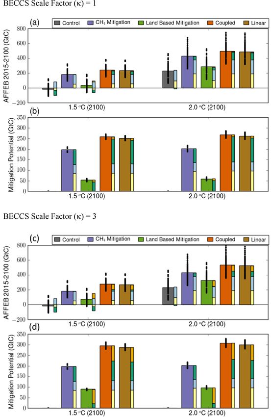
520                G. D. Hayman et al.: Regional variation in the effectiveness of methane-based climate mitigation options

                                                                        follows: (a) the 1.5 ◦ C profile uses 1Tlim = 1.5 ◦ C, µ0 = 0.1,
                                                                        and µ1 = 0.0, and (b) the 2 ◦ C profile uses 1Tlim = 2 ◦ C,
                                                                        µ0 = 0.08, and µ1 = 0.0.

                                                                        2.3     Scenarios and model runs

                                                                        We undertake a control run and other simulations with an-
                                                                        thropogenic CH4 mitigation or land-based mitigation, stabil-
                                                                        ising at either 1.5 ◦ C or 2.0 ◦ C warming without a tempera-
                                                                        ture overshoot. We denote the control run as “CTL” and the
                                                                        anthropogenic CH4 mitigation scenario, a land-based miti-
                                                                        gation scenario using BECCS, and a variant land-based sce-
                                                                        nario focussing on AR, as “CH4 ”, “BECCS”, and “Natural”,
                                                                        respectively. We also undertake runs combining the CH4 and
                                                                        land-based mitigation scenarios (coupled “BECCS + CH4 ”
                                                                        and coupled “Natural + CH4 ”) to determine if there are any
                                                                        non-linearities when we combine these mitigation scenarios.
                                                                        We summarise the key assumptions of these scenarios in Ta-
                                                                        ble 1.
                                                                           We use future projections of atmospheric CH4 concentra-
                                                                        tions and LULUC (specifically, the areas assigned to agri-
                                                                        culture and within that to BECCS) from the IMAGE SSP2
                                                                        projections (Doelman et al., 2018) as input or prescribed
                                                                        data for both the methane and land-based mitigation strate-
                                                                        gies (Table 1). This ensures that all projections are consis-
                                                                        tent and based on the same set of IAM model and socio-
                                                                        economic pathway assumptions. The SSP2 socio-economic
                                                                        pathway is described as “middle of the road” (O’Neill et
                                                                        al., 2017), with social, economic, and technological trends
                                                                        largely following historical patterns observed over the past
                                                                        century. Global population growth is moderate and levels off
Figure 3. Time series of key datasets used in the study. (a) The his-   in the second half of the century. The intensity of resource
toric temperature record (black) and the prescribed temperature pro-    and energy use declines. We define the upper and lower lim-
files used to represent warming of 1.5 ◦ C (blue) and 2 ◦ C (orange).   its of anthropogenic mitigation as the lowest (RCP1.9, de-
(b) The historic (black) and the projected non-CO2 greenhouse gas       noted “IM-1.9”) and highest (“baseline”, denoted “IM-BL”)
radiative forcing (W m−2 ) for the control (green) and methane mit-     total radiative forcing pathways, respectively, within the IM-
igation (purple) scenarios.                                             AGE SSP2 ensemble (Riahi et al., 2017). As described in
                                                                        Sect. 2.2.1, we modify the atmospheric concentrations of
                                                                        CH4 in the IMOGEN-JULES modelling, as the IMAGE sce-
sions of greenhouse gases and short-lived climate forcers,              narios assume constant natural and hence wetland methane
and, if necessary, capture atmospheric carbon. These profiles           emissions.
have the mathematical form of

1T (t) = 1T0 + γ t − 1 − e−µ(t)t γ t − (1TLim − 1T0 ) , (5)

                                                                        2.3.1    Methane: baseline and mitigation scenario

where 1T (t) is the change in temperature from pre-industrial           The anthropogenic CH4 emission increases from
levels at year t, 1T0 is the temperature change at a given              318 Tg yr−1 in 2005 to 484 Tg yr−1 in 2100 in the IM-
initial point (in this case 1T0 = 0.89 ◦ C for 2015), 1TLim is          AGE SSP2 baseline scenario but falls to 162 Tg yr−1 in 2100
the final prescribed warming limit, and                                 in the IMAGE SSP2 RCP1.9 scenario. The sectoral CH4
                                                                        emissions in 2005 (Energy Supply and Demand: 113;
µ(t) = µ0 + µ1 t and γ = β − µ0 (1TLim − 1T0 ) ,                 (6)    Agriculture: 136; Other Land Use (primarily burning): 18;
                                                                        Waste 52; all in Tg yr−1 ) are in agreement with the latest
where β (= 0.00128) is the current rate of warming and                  estimates of the global methane cycle (Saunois et al., 2020).
µ0 and µ1 are tuning parameters that describe anthropogenic             As summarised in Table S1 in the Supplement, the reduction
attempts to stabilise global temperatures (Huntingford et al.,          in CH4 emissions from specific source sectors is achieved as
2017). The parameter values used for the two profiles are as            follows: (a) “coal production” by maximising CH4 recovery

Earth Syst. Dynam., 12, 513–544, 2021                                                      https://doi.org/10.5194/esd-12-513-2021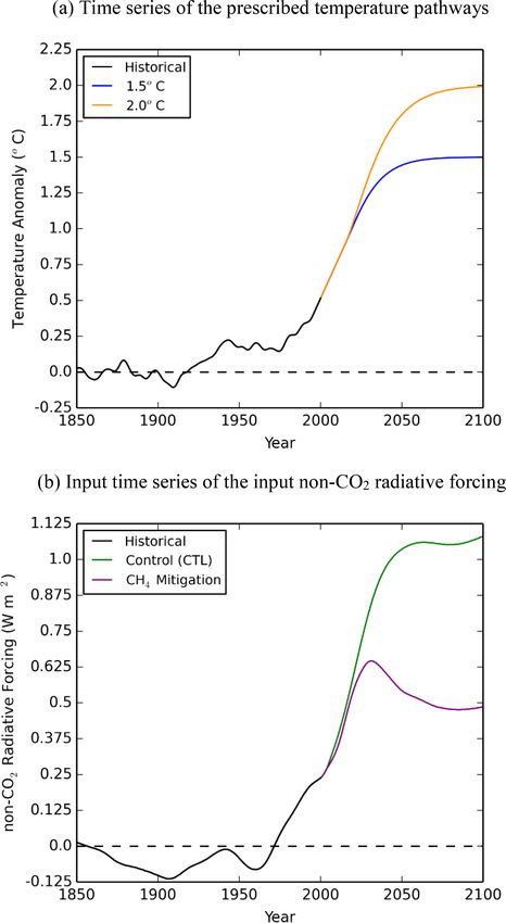
Table 1. The IMOGEN-JULES and post-processing scenario runs, key features, and the input and prescribed datasets used in the scenarios.

                                           (a) IMOGEN-JULES modelling scenarios (Note 1)
                                                Scenario (abbreviation)                                              Scenario-specific input and prescribed datasets (Notes 2, 3)
                                                Key features of the scenario
                                           1.   Control (“CTL”)                                                      Scenario-specific input data
                                                – Agricultural land accrued to feed growing populations              – Time series of radiative forcing by non-CO2 GHG and other non-CO2 climate forcers, for
                                                – No deployment of BECCS                                             SSP2 baseline scenario
                                                associated with the SSP2 pathway                                     – Time series of annual global atmospheric concentrations of CH4 and N2 O for the IMAGE
                                                – Anthropogenic CH4 emissions rise from 318 Tg yr−1 in 2005 to       Scenario-specific prescribed data
                                                484 Tg yr−1 in 2100                                                  the IMAGE SSP2 baseline scenario
                                                – Effects of the methane and carbon-climate feedbacks from           – Gridded annual time series of areas assigned to agriculture (crops and pasture), for the

https://doi.org/10.5194/esd-12-513-2021
                                                wetlands and permafrost thaw included                                IMAGE SSP2 baseline scenario, converted into fractions of the IMOGEN-JULES grid cell
                                           2.   Methane mitigation (“CH4 ”)                                          Scenario-specific input data
                                                – Agricultural land use as in Control (“CTL”) scenario               – Time series of radiative forcing by non-CO2 GHG and other non-CO2 climate forcers, for
                                                – Anthropogenic CH4 emissions decline from 318 Tg yr−1 in 2005       the IMAGE SSP2 RCP1.9 scenario
                                                to 162 Tg yr−1 in 2100, from the IMAGE SSP2 RCP1.9 scenario          – Time series of annual global atmospheric concentrations of CH4 and N2 O for the IMAGE
                                                – Effects of the methane and carbon–climate feedbacks from           SSP2 RCP1.9 scenario
                                                wetlands and permafrost thaw included                                Scenario-specific prescribed data
                                                                                                                     – As 1, gridded annual time series of area assigned to agriculture (crops and pasture) and
                                                                                                                     converted into fractions of the IMOGEN-JULES grid cell
                                           3.   Land-based mitigation, including BECCS (“BECCS”)                     Scenario-specific input data
                                                – Land use change based on the IMAGE SSP2 RCP1.9 scenario            – Time series of radiative forcing by non-CO2 GHG and other non-CO2 climate forcers, for
                                                – High levels of REDD and full reforestation                         the IMAGE SSP2 baseline scenario
                                                – Food-first policy so that bioenergy crops (BE) are only            – Time series of annual global atmospheric concentrations of CH4 and N2 O for the IMAGE
                                                implemented on land not required for food production                 SSP2 baseline scenario (as used in “CTL”)
                                                – Anthropogenic CH4 emissions as in Control (“CTL”) scenario         Scenario-specific prescribed data
                                                – Effects of the methane and carbon-climate feedbacks from           – Gridded annual time series of areas assigned to agriculture (crops and pasture) and within
                                                wetlands and permafrost thaw included                                that the area for bioenergy crops, for the IMAGE SSP2 RCP1.9 scenario and converted into a
                                                                                                                     fraction of the IMOGEN-JULES grid cell
                                           4.   Land-based mitigation with no BECCS (“Natural”)                      Scenario-specific input data
                                                – Land use as 3, except any land area allocated to bioenergy crops   – Time series of radiative forcing by non-CO2 GHG and other non-CO2 climate forcers, for
                                                is set to zero, allowing expansion of natural vegetation             the IMAGE SSP2 baseline scenario
                                                – Anthropogenic CH4 emissions as in Control (“CTL”) scenario         – Time series of annual global atmospheric concentrations of CH4 and N2 O for the IMAGE
                                                – Effects of the methane and carbon–climate feedbacks from           SSP2 baseline scenario (as used in “CTL”)
                                                                                                                                                                                                                       G. D. Hayman et al.: Regional variation in the effectiveness of methane-based climate mitigation options

                                                wetlands and permafrost thaw included                                Scenario-specific prescribed data
                                                                                                                     – Gridded annual time series of areas assigned to agriculture (crops and pasture). As 3, except
                                                                                                                     any land allocated to bioenergy crops is set to zero and converted into a fraction of the
                                                                                                                     IMOGEN-JULES grid cell

Earth Syst. Dynam., 12, 513–544, 2021
                                                                                                                                                                                                                       521
G. D. Hayman et al.: Regional variation in the effectiveness of methane-based climate mitigation options
https://doi.org/10.5194/esd-12-513-2021
Table 1. Continued.
(a) IMOGEN-JULES modelling scenarios (Note 1)
Scenario (abbreviation) Scenario-specific input and prescribed datasets (Notes 2, 3)
Key features of the scenario
5. Combined methane and land-based mitigation Scenario-specific input data
“Coupled (CH4 + BECCS)” – As in 2, time series of radiative forcing by non-CO2 GHG and other non-CO2 climate forcers,
– Combines CH4 mitigation of 2 with land-based mitigation for the IMAGE SSP2 RCP1.9 scenario
scenario of 3 – As in 2, time series of annual global atmospheric concentrations of CH4 and N2 O for the
IMAGE SSP2 RCP1.9 scenario
Scenario-specific prescribed data
– As in 3, gridded annual time series of areas assigned to agriculture (crops and pasture) and
within that the area for bioenergy crops, for the IMAGE SSP2 RCP1.9 scenario and converted
into prescribed fractions of the IMOGEN-JULES grid cell
6. Combined methane and land-based mitigation with no BECCS Scenario-specific input data
“Coupled (CH4 + Natural)” – As in 2, time series of radiative forcing by non-CO2 GHG and other non-CO2 climate forcers,
– Combines CH4 mitigation of 2 with land-based mitigation for the IMAGE SSP2 RCP1.9 scenario
scenario of 4 – As in 2, time series of annual global atmospheric concentrations of CH4 and N2 O for the
IMAGE SSP2 RCP1.9 scenario
Scenario-specific prescribed data
– As in 4, gridded annual time series of areas assigned to agriculture (crops and pasture) and
converted into a fraction of the IMOGEN-JULES grid cell
(b) Post-processing scenarios (Note 1)
Scenario Description of the scenario
Earth Syst. Dynam., 12, 513–544, 2021
“Abbreviation”
7. Optimisation of land-based mitigation Optimisation of scenarios 3 and 4 by selecting the scenario, which has the larger carbon
“Land-based mitigation: Optimised” uptake on a grid cell by grid cell basis
8. Optimisation of the combined methane and land-based mitigation Optimisation of scenarios 5 and 6 by selecting the scenario, which has the larger carbon
“Coupled Optimised” uptake on a grid cell by grid cell basis
Each scenario comprises two 136-member ensembles (34 GCMs × 2 ozone damage sensitivities × 2 methanogenesis Q10 temperature sensitivities): one for the 1.5 ◦ C warming target and another for the 2 ◦ C warming target.
All of the above scenarios also use time series of (1) observed temperature changes between 1850 and 2015, (2) profiles of temperature change between 2015 and 2100 to achieve the 1.5 and the 2 ◦ C warming targets, and
(3) the radiative forcing changes of non-CO2 radiative forcing between 1850 and 2015. We define (a) a “prescribed” dataset as one that is used unchanged in the IMOGEN-JULES modelling and (b) an “input” dataset as one
that provides the initial values that are subsequently changed.
522G. D. Hayman et al.: Regional variation in the effectiveness of methane-based climate mitigation options 523
from underground mining of hard coal; (b) “oil/gas produc- on natural grasslands in central Brazil, eastern and south-
tion and distribution” through control of fugitive emissions ern Africa, and northern Australia; Doelman et al., 2018).
from equipment and pipeline leaks and from venting during The IM-1.9 scenario also requires bioenergy crops to replace
maintenance and repair; (c) “enteric fermentation” through forests in temperate and boreal regions (notably Canada and
change in animal diet and the use of more productive animal Russia). The demand for bioenergy is linked to the carbon
types; (d) “animal waste” by capture and use of the CH4 price required to reach the mitigation target (Hoogwijk et al.,
emissions in anaerobic digesters; (e) “wetland rice produc- 2009). In this scenario, the area of land used for bioenergy
tion” through changes to the water management regime crops expands rapidly from 2030 to 2050, reaching a max-
and to the soils to reduce methanogenesis; (f) “landfills” by imum of 550 Mha in 2060 and then declining to 430 Mha
reducing the amount of organic material deposited and by by 2100. Table 2 gives the maximum area of BECCS de-
capture of any CH4 released; and (g) “sewage and wastew- ployed in each IMAGE region for the IM-1.9 scenario. This
ater” through using more wastewater treatment plants and defines the land use in the BECCS scenario.
also recovery of the CH4 from such plants and through more We define a third LULUC pathway, which is identical to
aerobic wastewater treatment. The levels of reduction vary the ”BECCS” scenario, except that any land allocated to
between sectors, from 50 % (agriculture) to 90 % (fossil fuel bioenergy crops is allocated instead to natural vegetation,
extraction and delivery). The abatement costs are between i.e. areas of natural land, which are converted to bioenergy
USD 300–1000 (1995 USD) (Table S1). Figure 4 presents crops, remain as natural vegetation, and areas that are con-
the IMAGE baseline and RCP1.9 CH4 emission pathways verted from food crops or pasture to bioenergy crops return
globally and for selected IMAGE regions, including the ma- to natural vegetation. We make no allowance for any changes
jor emitting regions of India, the USA, and China (Fig. S1 in the energy generation system, as this would require energy
in the Supplement shows the emission pathways for all sector modelling that is beyond the scope of this study. We
26 IMAGE regions). These two methane emission pathways denote this scenario as Natural. Table 2 also summarises the
(IMAGE SSP2 baseline and RCP1.9) define our CTL and main differences in land use between the BECCS and Natural
CH4 scenarios, respectively. scenarios for each IMAGE region.
Figure 5 presents time series of the land areas calculated
2.3.2 Land-based mitigation: baseline, BECCS, and
for trees and prescribed for agriculture (including bioenergy
Natural scenarios
crops) and bioenergy crops for the BECCS and Natural sce-
narios for the Russia and Brazil IMAGE regions, each as
For our land-based mitigation scenarios, we take time series a difference to the baseline scenario (IM-BL). Figure S2 is
of the annual areas assigned to agriculture (crops and pas- equivalent to Fig. 5 for all the IMAGE regions.
ture) and within that, the area allocated to bioenergy crops,
from the IM-BL and IM-1.9 scenarios (defined at the start of 2.3.3 Model runs
Sect. 2.3). We use the dynamic vegetation module in JULES
to calculate the evolution of the natural plant functional types For each temperature pathway (1.5 or 2.0 ◦ C) and for the
and the non-vegetated surface on the remaining land area in baseline and each mitigation scenario, the set of scenario runs
the grid cell (see Land use in Sect. 2.1). comprises a 136-member ensemble (34 GCMs × 2 ozone
The IM-BL LULUC scenario assumes (a) moderate land damage sensitivities × 2 methanogenesis Q10 temperature
use change regulation, (b) moderately effective land-based sensitivities). In all model runs, we include the effects of
mitigation, (c) the current preference for animal products, (d) the methane and carbon–climate feedbacks from wetlands
moderate improvement in livestock efficiencies, and (e) mod- and permafrost thaw, which we have shown previously to be
erate improvement in crop yields (Table 1 in Doelman et al., significant constraints on the AFFEBs (Comyn-Platt et al.,
2018). It represents a control scenario within which agri- 2018a).
cultural land is accrued to feed growing populations asso- As shown in Fig. 1, we use a number of input or prescribed
ciated with the SSP2 pathway and with no deployment of datasets: (a) time series of the annual area of land used for
BECCS. Three types of land-based climate change mitiga- agriculture, including that for BECCS if appropriate; (b) time
tion are implemented in the IMAGE land use mitigation series of the global annual mean atmospheric concentrations
scenarios (Doelman et al., 2018): (1) bioenergy, (2) reduc- of CH4 (and N2 O for the radiative forcing calculations of
ing emissions from deforestation and degradation (REDD or CO2 and CH4 ); (c) time series of the overall radiative forcing
avoided deforestation), and (3) reforestation of degraded for- by SLCFs and non-CO2 GHGs (corrected for the radiative
est areas. For the IM-1.9 scenario, there are high levels of forcing of CH4 ); and (d) time series of annual anthropogenic
REDD and full reforestation. The scenario assumes a food- CH4 emissions (used in the post-processing step). We take
first policy (Daioglou et al., 2019) so that bioenergy crops these from the IMAGE database for the relevant IMAGE
are only implemented on land not required for food produc- SSP2 scenario (baseline or SSP2-1.9). Table 1 lists the main
tion (e.g. abandoned agricultural crop land, most notably in scenario runs, their key features and the prescribed datasets
central Europe, southern China, and the eastern USA, and used (for agricultural land and BECCS, anthropogenic emis-
https://doi.org/10.5194/esd-12-513-2021 Earth Syst. Dynam., 12, 513–544, 2021524 G. D. Hayman et al.: Regional variation in the effectiveness of methane-based climate mitigation options Figure 4. Time series of annual methane emissions between 2005 and 2100 from all and selected anthropogenic sources according to the IMAGE SSP2 Baseline (solid lines) and SSP2-RCP1.9 (dotted lines) scenarios, globally and for selected IMAGE regions, with total emissions in black, energy sector in red, agriculture – cattle in blue, agriculture – rice in green, and waste in magenta. Note that the y axes have different scales for clarity. Earth Syst. Dynam., 12, 513–544, 2021 https://doi.org/10.5194/esd-12-513-2021
G. D. Hayman et al.: Regional variation in the effectiveness of methane-based climate mitigation options                                   525

Table 2. IMAGE regions, the maximum area of BECCS deployed (Mha), and the main differences in land use between the BECCS and
Natural scenarios.

 Region                    Abbreviation   Max. area of   Main land use difference between the BECCS and Natural scenarios
                                            bioenergy
                                          crops (Mha)
 Canada                    CAN                   65.9    Forest to BECCS in BECCS scenario
 USA                       USA                   39.0    Agricultural land and forest to BECCS (BECCS). Agricultural land to forest (Natural)
 Mexico                    MEX                    7.1    Agricultural land to BECCS and forest (BECCS). Agricultural land to forest (Natural)
 Central America           RCAM                   0.5    Little BECCS. Agricultural land to forests in both scenarios.
 Brazil                    BRA                   27.8    Agricultural land to BECCS and forest (BECCS). Agricultural land to forest (Natural)
 Rest of South America     RSAM                  20.3    Agricultural land to BECCS and forest (BECCS). Agricultural land to forest (Natural)
 Northern Africa           NAF                    0.0    No BECCS. No real differences between scenarios
 Western Africa            WAF                    3.1    Little BECCS. Agricultural land to forests in both scenarios.
 Eastern Africa            EAF                   33.9    Agricultural land to BECCS and forest (BECCS). Agricultural land to forest (Natural)
 South Africa              SAF                    1.0    Little BECCS. Agricultural land to forests in both scenarios.
 Rest of southern Africa   RSAF                  63.7    Agricultural land to BECCS and forest (BECCS). Agricultural land to forest (Natural)
 Western Europe            WEU                   23.6    Forest to BECCS in BECCS scenario
 Central Europe            CEU                   19.3    Forest to BECCS in BECCS scenario
 Turkey                    TUR                    0.0    No BECCS. No real differences between scenarios
 Ukraine region            UKR                   11.4    Forest to BECCS in BECCS scenario
 Central Asia              STAN                   0.7    Little BECCS. No real differences between scenarios
 Russia region             RUS                  146.1    Forest to BECCS in BECCS scenario
 Middle East               ME                     0.0    No BECCS. No real differences between scenarios
 India                     INDIA                  6.0    Forest to BECCS in BECCS scenario
 Korea region              KOR                    4.3    Forest to BECCS in BECCS scenario
 China                     CHN                   58.1    Forest to BECCS in BECCS scenario
 South East Asia           SEAS                  24.5    Forest to BECCS in BECCS scenario. Agricultural land to forest (Natural)
 Indonesia                 INDO                   0.0    No BECCS. Agricultural land to forests in both scenarios.
 Japan                     JAP                    2.7    Forest to BECCS in BECCS scenario
 Rest of South Asia        RSAS                   0.0    No BECCS. No real differences between scenarios
 Oceania                   OCE                   78.7    Forest to BECCS in BECCS scenario

sions and atmospheric concentrations of CH4 and the non-                         h                             i
CO2 radiative forcing).                                                  AFFEBi = C land (2100) − C land (2015)
   Figure 6 presents the effect of these scenarios on the mod-                                                   i
                                                                                + C ocean (2100) − C ocean (2015) i

elled atmospheric CH4 and CO2 concentrations. We adjust
the input atmospheric CH4 concentrations to allow for the                       + C atmos (2100) − C atmos (2015) i

interannual variability in the wetland CH4 emissions, as de-
                                                                                   + BECCS(2015 : 2100)i ,                                  (7)
scribed in Sect. 2.2.1. As we use the same input datasets for
the two warming targets, the major control on the modelled               where C land (t), C ocean (t), and C atmos (t) are the carbon stored
atmospheric CH4 concentrations is the CH4 emission path-                 in the land, ocean, and atmosphere, respectively, in year t
way followed, with the temperature pathway (1.5 ◦ C versus               and BECCS(t1 : t2 ) is the carbon sequestered via BECCS
2 ◦ C warming) having a minor effect. For CO2 , on the other             between the years t1 and t2 . The atmospheric carbon store
hand, the temperature and the CH4 emission pathways both                 does not include CH4 . This is a reasonable approximation,
lead to increased atmospheric CO2 concentrations, with the               however, given the relative magnitudes of the atmospheric
temperature pathway having a slightly larger effect.                     concentrations of CH4 (∼ 2 ppmv at the surface) and CO2
                                                                         (400 ppmv).
2.4     Post-processing                                                     Within the IMOGEN-JULES modelling framework, we
                                                                         use (a) the IMOGEN climate emulator to derive the changes
2.4.1    Anthropogenic fossil fuel emission budget and
                                                                         in the ocean and atmosphere carbon stores and (b) JULES
         mitigation potential
                                                                         for the changes in the land carbon store and carbon se-
Following Comyn-Platt et al. (2018a), we define the anthro-              questered through BECCS. We discuss the changes in the
pogenic fossil fuel CO2 emission budget (AFFEB) for sce-                 carbon stores for the baseline and different mitigation sce-
nario i as the change in carbon stores from present to the               narios in Sect. 3.1.
year 2100:

https://doi.org/10.5194/esd-12-513-2021                                                        Earth Syst. Dynam., 12, 513–544, 2021
526 G. D. Hayman et al.: Regional variation in the effectiveness of methane-based climate mitigation options
Figure 5. Time series of the land areas (in Mha) calculated for trees and prescribed for agriculture (including bioenergy crops) and bioenergy
crops for the BECCS (orange) and Natural (green), as a difference to the baseline scenario (IM-BL), for Brazil (a) and Russia (b) IMAGE
regions between 2000 and 2100. The dotted lines are the median and the spread the interquartile range for the 34 GCMs emulated and
4 factorial sensitivity simulations.
For brevity in the subsequent discussion, we use the fol- The key issue is that replacing natural vegetation with bioen-
lowing shorthand where the terms on the right-hand side ergy crops often results in large emissions of soil carbon and
of Eq. (7) are equivalent to those on the right-hand side of the loss of the benefits of maintaining forest carbon stocks.
Eq. (8): In such circumstances, Harper et al. (2018) find that the loss
of soil carbon in regions with high carbon density makes
AFFEBi = 1Ciland + 1Ciocean + 1Ciatmos + BECCSi . (8)
it difficult for BECCS to deliver a net negative emission of
We define the mitigation potential (MP) for a mitiga- CO2 . Hence, to optimise the land-based mitigation (LBM),
tion strategy, j , as the difference between a control AF- we compare the land carbon stocks in the BECCS and Natu-
FEB (AFFEBctl ) and the AFFEB resulting from applying the ral scenarios. We then select the optimum land management
strategy, i.e. option for each grid cell simulated as that which maximises
the AFFEB by year 2100, i.e.
MPj = AFFEBj − AFFEBctl , (9)
atmos ocean land
AFFEBLBM = 1CBECCS + 1CBECCS + 1CLBM , (11)
which can be broken down into its component parts as fol-
lows: with
MPj = MPland + MPocean + MPatmos
land
1CLBM =
j j j
grid cells
MPj = 1Cjland − 1Cctl
land
+ 1Cjocean − 1Cctl
ocean
P land
1CBECCS + BECCS land
where 1CBECCS land
< 1CBECCS + BECCS
l
or , (12)
gridPcells
+ 1Cjatmos − 1Cctl
atmos
+ BECCSj . (10)
land
1CNatural where land
1CNatural land
> 1CBECCS + BECCS
l
store
where 1Cscenario is the change in carbon between 2015
2.4.2 Optimisation of the land-based mitigation
and 2100 for the “store” (= atmosphere, ocean, or land) for
Harper et al. (2018) find that the land use pathways do not the LULUC scenario. We use the ocean and atmosphere con-
provide a clear choice for the preferred mitigation pathway. tributions from the BECCS simulations as the changes in
Earth Syst. Dynam., 12, 513–544, 2021 https://doi.org/10.5194/esd-12-513-2021You can also read