Sinking microplastics in the water column: simulations in the Mediterranean Sea
←
→
Page content transcription
If your browser does not render page correctly, please read the page content below
Ocean Sci., 17, 431–453, 2021
https://doi.org/10.5194/os-17-431-2021
This work is distributed under
the Creative Commons Attribution 4.0 License.

Sinking microplastics in the water column:
simulations in the Mediterranean Sea
Rebeca de la Fuente1 , Gábor Drótos1,2 , Emilio Hernández-García1 , Cristóbal López1 , and Erik van Sebille3,4
1 IFISC   (CSIC-UIB), Campus Universitat de les Illes Balears, Palma de Mallorca, Spain
2 MTA–ELTE      Theoretical Physics Research Group, Budapest, Hungary
3 Institute for Marine and Atmospheric Research, Utrecht University, Utrecht, the Netherlands
4 Centre for Complex Systems Studies, Utrecht University, Utrecht, the Netherlands

Correspondence: Emilio Hernández-García (emilio@ifisc.uib-csic.es)

Received: 28 September 2020 – Discussion started: 19 October 2020
Revised: 27 January 2021 – Accepted: 27 January 2021 – Published: 9 March 2021

Abstract. We study the vertical dispersion and distribution of     Kooi et al., 2017) or sinking (Erni-Cassola et al., 2019), but
negatively buoyant rigid microplastics within a realistic cir-     also wind-driven mixing presumably leads to an underesti-
culation model of the Mediterranean sea. We first propose an       mation for the amount of particles remaining close to the
equation describing their idealized dynamics. In that frame-       sea surface (Kukulka et al., 2012; Enders et al., 2015; Suaria
work, we evaluate the importance of some relevant physi-           et al., 2016; Poulain et al., 2018). The distribution of plas-
cal effects (inertia, Coriolis force, small-scale turbulence and   tic pollution in the sea is poorly understood at present but
variable seawater density), and we bound the relative error        would be crucial to properly evaluate the exposure of marine
of simplifying the dynamics to a constant sinking velocity         biota to this material and formulate strategies for cleaning the
added to a large-scale velocity field. We then calculate the       oceans (Horton and Dixon, 2018).
amount and vertical distribution of microplastic particles on         Floating plastics and those that have beached or sedi-
the water column of the open ocean if their release from the       mented on the seafloor are relatively well studied through
sea surface is continuous at rates compatible with observa-        field campaigns (although an explanation is missing for many
tions in the Mediterranean. The vertical distribution is found     findings; Andrady, 2017; Erni-Cassola et al., 2019; Kane and
to be almost uniform with depth for the majority of our pa-        Clare, 2019). In contrast, the presence of plastics within the
rameter range. Transient distributions from flash releases re-     water column has received less attention, and many surveys
veal a non-Gaussian character of the dispersion and various        in this realm are restricted to so-called underway samples,
diffusion laws, both normal and anomalous. The origin of           a few meters below the surface (e.g., Enders et al., 2015).
these behaviors is explored in terms of horizontal and verti-      However, for example, Choy et al. (2019) reported that be-
cal flow organization.                                             low the mixed layer and down to 1000 m depth in Monterey
                                                                   Bay, concentrations of plastics are larger than at the surface
                                                                   (Thompson et al., 2004; Hidalgo-Ruz et al., 2012). Egger
                                                                   et al. (2020) found more plastic between 5 and 2000 m below
1   Introduction                                                   the North Pacific Garbage Patch than at the surface. These
                                                                   findings turn out to mostly concern plastic pieces that, ac-
Approximately 8 million tonnes of plastics end up in the           cording to their nominal material density, would be classified
oceans every year (Jambeck et al., 2015). Nevertheless, only       as positively buoyant (Egger et al., 2020).
a very small percentage, around 1 %, remains on the surface           In this paper, we focus on a certain class of plastic
(van Sebille et al., 2015; Choy et al., 2019). The rest leaves     particles, negatively buoyant rigid microplastics, excluding
the surface of the ocean (Ballent et al., 2013; van Sebille        very small sizes, and we estimate their vertical distribution
et al., 2020) through beaching (Turner and Holmes, 2011),          through the water column and their amount in the Mediter-
biofouling (Ye and Andrady, 1991; Chubarenko et al., 2016;

Published by Copernicus Publications on behalf of the European Geosciences Union.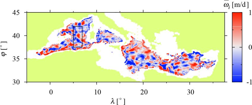
432                                                          R. de la Fuente et al.: Sinking microplastics in the water column

ranean Sea. Microplastic particles are among the most im-           and Morales Maqueda, 2019; Wichmann et al., 2019; Soto-
portant contributors to marine plastic pollution (Arthur et al.,    Navarro et al., 2020). This suggests that reverse processes
2009). Closely following the work of Monroy et al. (2017)           could also take place after biofouling and that the dynam-
for sinking biogenic particles but choosing particle proper-        ics of such particles is complicated (Kooi et al., 2017; Erni-
ties to correspond to those of negatively buoyant microplas-        Cassola et al., 2019).
tics, we first justify the use of a simplified equation of mo-         Particles denser than seawater dominantly accumulate at
tion, in which the plastic particle velocity is the sum of the      the sea bottom (Mountford and Morales Maqueda, 2019). A
ambient flow velocity and a sinking velocity depending on           mechanism by which microplastics denser than water can
particle and water characteristics. In particular, we estimate      also be present within the water column is the finite time
the impact of some corrections to this simple dynamics and          taken by them to reach the bottom. Under continuous release
evaluate in detail the influence of the spatial variation of the    at the surface and sedimentation at the bottom, the transient
seawater density on the plastic dispersion and sinking charac-      falling would lead to a steady distribution for the amount of
teristics. For our Mediterranean case study, the impact of the      plastic in the water column at any given time, and this dis-
varying seawater density on particle trajectories can be com-       tribution has never been estimated. Note that the Eulerian
parable to the estimated effect of the neglected small scales       methodology of Mountford and Morales Maqueda (2019),
below the hydrodynamical model’s resolution.                        treating sedimentation (i.e., deposition on the seafloor) by
   We then estimate the amount of microplastic particles in         parametrization and thus leaving particles in the water col-
the water column of the open Mediterranean. Our estimates           umn indefinitely long, is not suitable for this estimation. One
rely on a uniform vertical distribution, which is confirmed         aim of this paper is to explore this distribution by means of
by our numerical simulations to be a good approximation             Lagrangian simulations.
for fast-sinking particles. This can be explained by a sim-            There are different classes of microplastic particles denser
ple model in which released particles sink with a constant          than seawater. For example, dense synthetic microfibers have
velocity. Detailed consideration of the transient dynamics          been found to strongly dominate in sediment samples far
identifies small non-Gaussian vertical dispersion around this       from the coast (Woodall et al., 2014; Fischer et al., 2015;
simple sinking behavior, with transitions between anomalous         Bergmann et al., 2017; Martin et al., 2017; Peng et al., 2018)
and normal effective diffusion.                                     and have been detected in large proportions in deep-water
                                                                    samples and sediment traps in the open sea as well (Bagaev
                                                                    et al., 2017; Kanhai et al., 2018; Peng et al., 2018; Reinec-
2   Types of microplastics in the water column                      cius et al., 2020). With these mostly originating from land-
                                                                    based sources (Dris et al., 2016; Carr, 2017; Gago et al.,
The dynamics and the fate of microplastics in the ocean are         2018; Wright et al., 2020), it is not obvious to explain their
largely determined by their material density (Erni-Cassola          abundance on abyssal oceanic plains (Kane and Clare, 2019).
et al., 2019). However, shape, size and rigidity are also rele-     Maritime-activity sources (Gago et al., 2018) can contribute
vant properties, characteristic transport pathways to the water     to that. Another reason could be that their special and de-
column being different for different particle types.                formable shape results in a strongly reduced settling veloc-
   Typically, positively buoyant plastic types will remain          ity (Bagaev et al., 2017) that allows long-distance horizontal
floating at the sea surface or close to it and then will not        transport (Nooteboom et al., 2020). In any case, it is difficult
contribute to the microplastic content in the water column,         to estimate the amount of microfibers in the oceans due to
the topic we are interested in this paper. However, it has          sampling issues and to their absence from statistics of mis-
been documented experimentally that biofouling may in-              managed plastic waste (Carr, 2017; Barrows et al., 2018),
crease sinking rates of particles up to 81 % and enhances           and we will not consider them further in this paper. We also
sedimentation (Kaiser et al., 2017). So, a class of high abun-      disregard films, which are only sporadically encountered in
dance and mass may be represented by nearly neutrally buoy-         the open ocean (Bagaev et al., 2017) and thus have moderate
ant microplastic particles that are generated by biofouling         importance.
(Ye and Andrady, 1991; Chubarenko et al., 2016) from pos-              We concentrate in the following on dense rigid microplas-
itively buoyant plastic types or by other mechanisms of ag-         tic particles. The most abundant particles of this class are
gregation with organic matter, especially for small particle        fragments (e.g., Martin et al., 2017; Peng et al., 2018), which
sizes (Kooi et al., 2017).                                          have an irregular shape, but their extension is usually compa-
   In fact, the fallout from the North Pacific Garbage Patch        rable in the three dimensions. Experimental estimates for the
almost entirely consists of plastic types nominally less dense      settling velocities of irregular fragments or other nonspher-
than water (Egger et al., 2020). Although some of these             ical particles have suggested considerable deviations from
immersed particles finally reach the sea bottom, their pro-         values predicted by the Stokes law (Kowalski et al., 2016;
portion in sedimented plastic is minor except for the im-           Khatmullina and Isachenko, 2017; Kaiser et al., 2019), so
mediate vicinity of coasts where water is shallow. Most             that it is unclear how a precise full equation of motion should
of these particles remain in the photic zone (Mountford             be constructed. For a qualitative exploration of particle trans-

Ocean Sci., 17, 431–453, 2021                                                           https://doi.org/10.5194/os-17-431-2021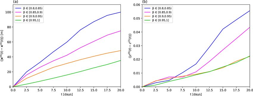
R. de la Fuente et al.: Sinking microplastics in the water column                                                               433

port through the water column, we will argue in Sect. 4.1 and       microlayer where surface tension keeps them floating (Song
Appendix A that the Maxey–Riley–Gatignol (MRG) equa-                et al., 2014). The range of horizontal transport of these parti-
tion (Maxey and Riley, 1983) should be appropriate for a            cles at the sea surface is unclear but expected to be restricted
reasonably wide range of such particles.                            to short distances because sinking from the sea surface mi-
   Whatever their precise equation of motion is, these sink-        crolayer is considerable, especially in waters disturbed by
ing particles (directly detected by Bagaev et al., 2017, and        waves (Hardy, 1982; Stolle et al., 2010).
Peng et al., 2018) are thought to reach the seafloor relatively        While the idea of Kooi and Koelmans (2019) to treat all
fast (Chubarenko et al., 2016; Kane and Clare, 2019; Soto-          plastic particles together by means of continuous distribu-
Navarro et al., 2020), landing within horizontal distances of       tions is appealing, the above considerations strongly favor
tens of kilometers from their surface location of release (see      the separate treatment of positively buoyant pieces, nega-
Sect. 4.2 and Appendix B). One consequence of their fast            tively buoyant microfibers and negatively buoyant rigid par-
sinking is the absence of almost any fragmentation after they       ticles of sufficiently big size, since these classes have very
leave the sea surface (Andrady, 2015; Corcoran, 2015), and          different dynamics and sources. In the following we concen-
the influence of biological processes on the particles’ prop-       trate on the properties, amount and dynamics of particles of
erties should also be moderate, leaving their size and shape        the last class.
intact during sinking. Note that, in contrast to the case of
floating plastics (Kooi et al., 2017; Kvale et al., 2020), inter-
action of sinking plastics with particulate matter of biolog-       3     Considerations for modeling negatively buoyant
ical origin appears to be moderate. This is according to the              rigid microplastics
absence of a need to disassemble microplastic pieces from
biological aggregates during sample processing as described         3.1    Physical properties
by Bagaev et al. (2017). Note, however, that experimental re-
sults by Michels et al. (2018) indicate that aggregation with       From a meta-analysis of 39 previous studies, Erni-Cassola
organic material might occur within a sufficiently short time       et al. (2019) established the proportion of the most abundant
at surface layers, which would likely lead to increased sink-       polymer types discharged into water bodies: PE (polyethy-
ing velocities (Long et al., 2015). Transport by bottom cur-        lene, 23 %), PP (polypropylene, 13 %), PS (polystyrene, 4 %)
rents (Kane and Clare, 2019; Kane et al., 2020) is important        and PP&A (group of polymer types formed by polyesters,
for explaining their distribution in sediments after coastal re-    PEST; polyamide, PA; and acrylics, 13 %). Note that these
lease. However, the statements above imply that the dense           proportions do not distinguish between different regions
rigid microplastic content of samples from deep-sea trenches        (e.g., coastal region or open water; even inland water bod-
and abyssal plains (van Cauwenberghe et al., 2013; Fischer          ies of urban environments are included in the analysis) and
et al., 2015; Peng et al., 2018; Kane and Clare, 2019) must         between the particle types (size range and shape) concerned
originate from sources at the surface of the open sea rather        in the different studies. We organize these polymer types
than from coastal inputs.                                           according to their density (Chubarenko et al., 2016; An-
   While methodological issues make the quantification of           drady, 2017; Erni-Cassola et al., 2019) in Fig. 1: PP between
abundance difficult (Song et al., 2014; Andrady, 2015;              850–920 kg/m3 , PE of 890–980 kg/m3 , PS of 1040 kg/m3
Filella, 2015; Lindeque et al., 2020), negatively buoyant mi-       (excluding its foamed version), PEST in the range 1100–
croplastic fragments have indeed been found in surface and          1400 kg/m3 , PA within 1120–1150 kg/m3 and acrylic of
near-surface samples of the open waters of the Mediterranean        1180 kg/m3 . There is also some less abundant plastic like
Sea (Suaria et al., 2016) and the Atlantic Ocean (Enders            polytetrafluoroethylene (PTFE) which has higher densities,
et al., 2015), respectively, from which they can contribute to      in the range 2100–2300 kg/m3 .
microplastic content of the water column and deep-sea sedi-            Thus, the full range of microplastic particle densities in
ments (Fischer et al., 2015; Bagaev et al., 2017). Horizontal       the ocean, denoted here as ρp , is 850–2300 kg/m3 , and most
transport of these particles can be carried out by marine or-       of them have densities within the interval 850–1400 kg/m3 .
ganisms, and spontaneous attachment to pieces of positive           This has to be compared with the seawater density, which
buoyancy is a further possibility but is not yet discussed in       close to the surface has a conventional mean value of ρf =
the literature. Composite pieces of debris or those that con-       1025 km/m3 (red line in Fig. 1) and changes around 1 % from
tain trapped air (including foams in some cases) may also           the surface to the sea bottom. Since we are interested in sink-
represent a source of microplastic ending at the water col-         ing material, and for the sake of maximal practicality, we
umn (Andrady, 2015). However, most of such particles are            restrict our study to microplastics of densities 1025 kg/m3 <
presumably released by local maritime activity. An exam-            ρf < 1400 kg/m3 .
ple of this are flakes of paint and structural material from           Another relevant property of plastic particles is their size.
boats and ships, which contain negatively buoyant alkyds            By a widely accepted definition, microplastics are particles
and poly(acrylate/styrene). Despite the particle’s high den-        with a diameter less than 5 mm without any lower limit
sity, large amounts of them may be found in the sea surface         (Arthur et al., 2009). Some observations at the ocean sur-

https://doi.org/10.5194/os-17-431-2021                                                            Ocean Sci., 17, 431–453, 2021
434                                                           R. de la Fuente et al.: Sinking microplastics in the water column

                                                                     will discuss in Sect. 4.1, this radius is well within the validity
                                                                     range of the MRG equation.

                                                                     3.2    Source estimation

                                                                     In this subsection we indicate the total amount of dense mi-
                                                                     croplastics entering the water column in open waters of the
                                                                     Mediterranean. Despite the correlation of plastic source with
                                                                     coastal population density, the rapid fragmentation of small
                                                                     particles along the shoreline (Pedrotti et al., 2016) and the
                                                                     seasonal variability of spatial distribution of floating parti-
                                                                     cles (Macias et al., 2019), we focus on local maritime activity
                                                                     and exclude direct release from surface accumulation areas
                                                                     or the coast, either from urban areas or from rivers. The es-
                                                                     timations are based on the results of Kaandorp et al. (2020).
                                                                     They provide a total amount of yearly plastic release into the
Figure 1. Polymer densities for the most abundant microplastics      Mediterranean in the range 2200–4000 t, from which around
identified in water bodies (Erni-Cassola et al., 2019).              37 % corresponds to negatively buoyant plastic, and 6 % are
                                                                     due to maritime activity. This 37 % agrees well with previous
                                                                     global estimations (Lebreton et al., 2018).
                                                                        We will take these numbers, 4000 t per year, 37 % of sink-
face show that the most common diameter is around 1 mm               ing particles and the proportion of direct release by maritime
(Cózar et al., 2014, 2015), with an exponential decay with           activity (6 %), to obtain in Sect. 4.3 an estimate for the basin-
increasing diameter up to 100 mm. However, the absence of            wide yearly release of negatively buoyant sphere-like mi-
this peak in other studies that show an increasing abundance         croplastics in the open Mediterranean. Note that we choose
with further decreasing size (Enders et al., 2015; Suaria et al.,    the upper bound, 4000 t per year, in order to account for the
2016; Erni-Cassola et al., 2017) suggests (Song et al., 2014;        considerable amount of unregistered particles.
Andrady, 2015; Erni-Cassola et al., 2017; Bond et al., 2018;
                                                                     3.3    Dynamics
Lindeque et al., 2020) the need for new technologies in sam-
pling methods (which usually use trawl nets with a mesh size         A standard modeling approach (Siegel and Deuser, 1997;
around 0.3 mm) and especially for the adaptation of care-            Monroy et al., 2017; Liu et al., 2018; Monroy et al., 2019) for
ful and standardized analysis procedures to avoid artifacts          the transport of noninteracting sinking particles is to consider
(Filella, 2015).                                                     the time-dependent particle velocity v as the combination of
   Field data about distributions of size and quantifiers of         the ambient fluid flow u and a settling velocity v s as
shape for negatively buoyant rigid particles in the water col-
umn or deep-sea sediments are not available to date to the           v = u + vs ,                                                  (1)
best of our knowledge, except in the Arctic from Bergmann
et al. (2017). However, their results may not apply to the ma-       with
jority of the oceans because of the very special dynamics pro-
vided by melting and freezing of sea ice (Bergmann et al.,                                       3ρf                     a2
                                                                     v s = (1 − β)gτp , β =                and τp =         .      (2)
2017). Data from Bergmann et al. (2017) and Song et al.                                        2ρp + ρf                 3βν
(2014) about unspecified sedimented fragments and paint
                                                                     g denotes the gravitational acceleration vector, pointing
particles, respectively, exhibit an increasing abundance with
                                                                     downwards; β is a parameter depending on the particle and
decreasing size, most particles being smaller than 0.05 mm.
                                                                     the fluid densities, ρp and ρf , respectively. Particles heavier
Laboratory findings about surface degradation of individual
                                                                     than water have β < 1, and β = 1 for neutrally buoyant parti-
particles also indicate such a tendency (Song et al., 2017).
                                                                     cles. The expression given for β assumes spherical particles.
Thus, these findings seem to indicate the prominent presence
                                                                     τp is the Stokes time, i.e., the characteristic response time of
of small pieces of plastic. Nevertheless the observations of
                                                                     the particle to changes in the flow, where a is the radius of the
Bagaev et al. (2017), Kanhai et al. (2018) and Peng et al.
                                                                     particle and ν the kinematic viscosity of the fluid. Although
(2018) do not indicate this abundance of small particles.
                                                                     Eq. (1) is commonly used, we are not aware of a systematic
   For these reasons, we will disregard particles of extremely
                                                                     justification of it in the microplastics context. This will be
small size. To keep our qualitative study sufficiently simple,
                                                                     done in Sect. 4.1.
we will consider all our modeled particles to have a radius
a = 0.05 mm (a diameter of 0.1 mm). This is a rather small
size, but still within the commonly measured ranges. As we

Ocean Sci., 17, 431–453, 2021                                                             https://doi.org/10.5194/os-17-431-2021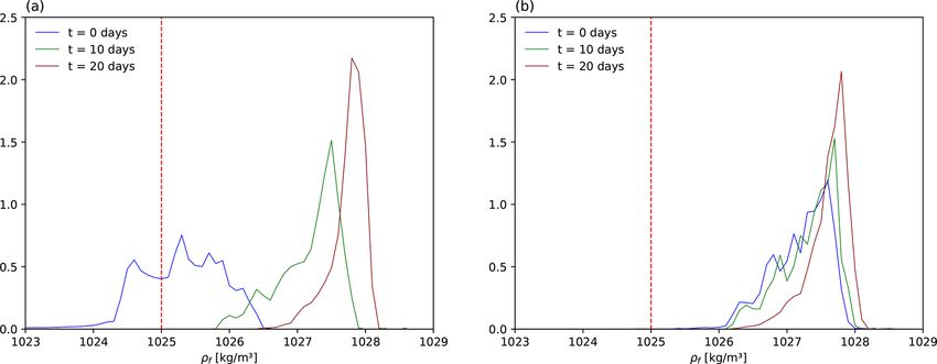
R. de la Fuente et al.: Sinking microplastics in the water column                                                                  435

3.4    Numerical procedures                                          range of validity of Eq. (3) assuming ν = 1.15 × 10⁻⁶ m2 /s
                                                                     and ρf = 1025 kg/m3 to be fixed. This gives β in the range
For the flow velocity u we use a 3D velocity field from              0.8–1. The possibility of small changes in the seawater den-
NEMO (Nucleus for European Modelling of the Ocean),                  sity as the particle sinks, which translates to variations in v s ,
which implements a horizontal resolution of 1/12◦ and 75             will also be analyzed in Sect. 4.2.
s levels in the vertical with data updated every 5 d (Madec,            In Fig. 2 we show a diagram with the settling velocities
2008; Madec and Imbard, 1996). Salinity and temperature              and particle sizes for which Eq. (3) is valid. We plot the min-
are also extracted from that model. The Parcels Lagrangian           imal value of the Kolmogorov scale η = 0.3 mm with the red
framework (Delandmeter and van Sebille, 2019) is used to in-         line (Jiménez, 1997), and Rep = 1 with a black line, which
tegrate the particle trajectories from Eq. (1) or more complex       bound the area of validity (shaded in the plot). We also in-
ones to be considered in Sect. 4.1. Typical numerical exper-         dicate vs as a function of a for β = 0.8 with the blue curve,
iments to obtain the results presented below consist of dis-         corresponding to the upper bound to vs for typical microplas-
tributing a large number N of particles in a horizontal layer        tic densities. In total, the zone with light shading in Fig. 2
over the whole Mediterranean on the nodes of a sinusoidal-           represents a parameter region where Eq. (3) applies for parti-
projection grid (Seong et al., 2002), so that their release is       cles with β < 0.8 (i.e., particles falling faster than the typical
with uniform horizontal density. We locate this input source         ones), whereas the area of our interest, corresponding to β ≥
at 1 m depth to avoid surface boundary conditions. After par-        0.8, is represented by dark shading, denoting the typical plas-
ticles are released at some initial date, in a so-called flash re-   tic sizes and corresponding settling velocities for which the
lease, they evolve under equations of motion such as Eq. (1),        equation is valid. As a rule of thumb, in a typical situation,
and the statistics of the resulting particle cloud are analyzed.     validity of Eq. (3) requires vs < 0.01 m/s and a < 0.3 mm. As
                                                                     discussed in Sect. 3.1, information about particles in the va-
                                                                     lidity range is particularly sparse for surface waters because
4     Results                                                        of the usual sampling techniques, but sediment data indicate
                                                                     the prevalence of sufficiently small particles. Furthermore, in
4.1    Range of validity of Eq. (1)
                                                                     sufficiently calm waters, the Kolmogorov scale is larger (of
We next show, closely following the treatment of Monroy              the order of millimeters; Jiménez, 1997), so that a can be
et al. (2017) for biogenic particles, that possible inertial ef-     increased to this size without compromising the equation va-
fects that would correct Eq. (1) are negligible for the sizes        lidity. In any case, these estimates of the Kolmogorov scale
and densities of typical dense microplastics. To this end, sim-      assume wind-driven turbulence and are thus restricted to the
ilarly to many other studies (Michaelides, 2003; Balkovsky           mixed layer (Jiménez, 1997), below which η is undoubtedly
et al., 2001; Cartwright et al., 2010; Haller and Sapsis, 2008),     larger. Deviations from a spherical shape may lead to a more
we start by choosing the simplified standard form of the             complicated motion than that described by the MRG equa-
more fundamental Maxey–Riley–Gatignol (MRG) equation                 tion, especially through particle rotation (Voth and Soldati,
(Maxey and Riley, 1983) and analyze under which conditions           2017). In Appendix A, we present quantitative arguments for
it is valid for microplastic transport. After finding the MRG        the applicability of the MRG equation to rigid microplastic
equation to be valid for an important range of microplastic          particles of common shapes in the parameter ranges of our
particles, we will explore its relationship with Eq. (1).            interest.
    The simplified MRG equation gives the velocity v(t) of a            The simplified MRG equation, Eq. (3) thus represents an
very small spherical particle in the presence of an external         appropriate basis for qualitative estimations of the transport
flow u(t) as                                                         properties of negatively buoyant rigid microplastics in the
                                                                     water column. Note that rigidity of the particles is an essen-
dv    Du u − v + v s                                                 tial condition which is why the advection of microfibers is
   =β    +           .                                        (3)    out of the scope of this paper.
dt    Dt     τp
                                                                        The connection between Eq. (3) and its approximation
Beyond sphericity, two conditions are needed for the validity        Eq. (1) is made by noticing that τη ≈ 1 s in the ocean (Mon-
of Eq. (3) (Monroy et al., 2017; Maxey and Riley, 1983): (a)         roy et al., 2017; Jiménez, 1997), so that the Stokes number
the particle radius, a, has to be much smaller than the Kol-         St = τp /τη , which measures the importance of particle iner-
mogorov length scale η of the flow, which has values in the          tia in a turbulent flow, is very small (of the order of 10−3 –
range 0.3 mm < η < 2 mm for wind-driven turbulence in the            10−2 ). Thus an expansion of the MRG equation for small St
upper ocean (Jiménez, 1997); (b) the particle Reynolds num-          (smallness of the Froude number, i.e., smallness of fluid ac-
ber Rep = a|v−u|ν    ≈ avν s should satisfy Rep  1. Note that       celerations with respect to gravity, is also required) can be
this last condition imposes restrictions on the values of the        performed. The expansion in its simplest form leads to (Bal-
particles’ density and size, partially via the settling velocity     achandar and Eaton, 2010; Monroy et al., 2017; Drótos et al.,
vs = |v s |. For the most abundant sinking microplastics, i.e.,      2019)
with densities ρp = 1025–1400 kg/m3 , we now determine the

https://doi.org/10.5194/os-17-431-2021                                                               Ocean Sci., 17, 431–453, 2021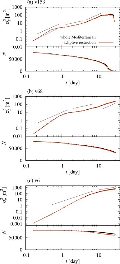
436                                                               R. de la Fuente et al.: Sinking microplastics in the water column

                                                                         for a small-scale flow (Monroy et al., 2017; Kaandorp et al.,
                                                                         2020). Results similar to those by Monroy et al. (2017), sum-
                                                                         marized in Appendix B, indicate that after 10 d of integration
                                                                         the relative difference between particle positions given by
                                                                         Eq. (4) with and without this “noise” term modeling small
                                                                         scales (using β = 0.99) is around 8 % for the horizontal dis-
                                                                         placements and 5 % for the vertical ones. The figures be-
                                                                         come 12 % and 5 %, respectively, when evolving the particles
                                                                         for 20 d. These errors are moderate, although they may be
                                                                         of importance under some circumstances (Nooteboom et al.,
                                                                         2020). We consider these figures as a baseline to evaluate cor-
                                                                         rections to the simple Eq. (1): adding more complex particle-
                                                                         dynamics terms to it will not improve plastic-sedimentation
                                                                         modeling unless the effect of these corrections is signifi-
Figure 2. Settling velocities and particle sizes for which Eq. (3)       cantly larger than the above estimations for the effect of the
holds. Kolmogorov scale is represented by the red line and Rep = 1       unknown small-scale flow. In the following we consider the
with a black line, which bound the area of validity. Blue curve cor-     simple Eq. (1), but we estimate the implications of assuming
responds to vs = vs (β, a) for β = 0.8, the upper bound to vs for typ-   or not assuming a constant value of the water density.
ical microplastic densities. Dark shading denotes the plastic particle
sizes and corresponding settling velocities for which application of
Eq. (3) is valid.
                                                                         4.2   Effect of variable seawater density

                                                                         In this section we analyze the role of a variable seawater den-
                                                                         sity on the particle settling dynamics. Fluid density is calcu-
                                                                         lated from the TEOS-10 equations, which is a thermodynam-
                           Du
v ≈ u + v s + τp (β − 1)      .                                   (4)    ically consistent description of seawater properties derived
                           Dt                                            from a Gibbs function, for which absolute salinity is used
   We can now take the results of Monroy et al. (2017) for               to describe salinity of seawater and conservative tempera-
biogenic particles of sizes and densities similar to the mi-             ture replaces potential temperature (Pawlowicz, 2010). In the
croplastics considered here to show that the inertial correc-            simulations described in this section, as particles move in the
tions (the term proportional to τp ) in Eq. (4) are negligible,          ocean they encounter different temperatures and salinities, as
so that the simpler Eq. (1) correctly describes sinking of mi-           given by the NEMO model described in Sect. 3.4, and then
croplastics in the considered parameter range. For complete-             they experience different values of the ambient-fluid density.
ness, we report in Appendix B the explicit numerical cal-                   We consider particles of a fixed density ρp =
culations showing this (in which the influence of the Corio-             1041.5 kg/m3 . This implies that for a nominal water
lis force is also taken into account, since it is known to be            density of ρf = 1025 kg/m3 the value of β would be
of the same order as or larger than the inertial term when a             β = 0.99, giving a sinking velocity vs = 6.2 m/d for our
large-scale flow is used for u). In particular we find, from             particles of radius a = 0.05 mm, but this sinking velocity
experiments of releasing particles with β in the range 0.8–1             will be increased or decreased in places where water density
from 1 m below the surface in the whole Mediterranean, that              is lower or higher, respectively, so that we have a spatially
differences in horizontal particle positions between the dy-             and temporally dependent velocity in Eq. (1). The particle
namics of Eq. (4) and Eq. (1) after 10 d of integration are just         density and size have been chosen to be representative of the
0.26 % of the horizontal displacements. For the vertical mo-             slowly sinking microplastic particles, for which we expect
tions the difference is of about 0.05 %. Thus, Eq. (1) provides          the seawater density variations to have the largest impact. In
a proper description of the dynamics.                                    this way we find some upper bound for the importance of
   Even if an equation of motion is accurate, the accuracy of            variability in seawater density for particle trajectories.
its solution is limited by that of the input data. In particu-              We release N = 78 803 particles over the whole Mediter-
lar, small-scale flow features are absent from oceanic veloc-            ranean Sea and monitor their trajectories under Eq. (1). Fig-
ity fields u simulated on large-scale domains, which is an               ure 3a shows the histogram of water densities encountered by
important limitation of the respective solutions of Eq. (1).             the particles when the release is performed on 8 July 2000.
The NEMO velocity field of our choice is not an exception,               On this summer date, the Mediterranean is well stratified,
but a rigorous evaluation of the corresponding errors of par-            at least in its upper layers. Initially the particles are in sur-
ticle trajectories is not possible without knowing the actual            face waters with a range of salinities that average approxi-
small-scale flow. Nevertheless, one can roughly estimate the             mately to the nominal ρf = 1025 kg/m3 . But as they sink in
effect of these small scales by adding a stochastic term to              time they reach layers with higher densities (and more ho-
Eq. (1) with statistical properties similar to the expected ones         mogeneous across the Mediterranean). When the release is

Ocean Sci., 17, 431–453, 2021                                                                 https://doi.org/10.5194/os-17-431-2021
R. de la Fuente et al.: Sinking microplastics in the water column 437
Table 1. Relative effect on horizontal and vertical particle positions variable density on particles that sink faster will be smaller.
after 10 and 20 d of integration, averaged over 78 803 particles re- Also, the effects reported in Table 1 remain of the order of the
leased over the whole Mediterranean at 1 m depth, of replacing the estimations of the effects of unresolved small scales of the
actual seawater density by a nominal value ρf = 1025 kg/m3 . flow (Sect. 4.1). As a consequence, in the following we will
not consider variable seawater density, but restrict our mod-
10 d 20 d eling to Eq. (1) with a constant nominal value of the sinking
Horizontal: 1.12 % 2.75 % velocity vs .
Summer release
Vertical: 3.19 % 6.25 %
4.3 Total mass and vertical distribution of
Horizontal: 1.88 % 5.62 %
Winter release
Vertical: 8.14 % 9.32 %
microplastics
We will first estimate the total mass of negatively buoyant
rigid microplastics in the water column of the open Mediter-
done in winter (Fig. 3b) the water column is more mixed, so ranean Sea by assuming a uniform vertical distribution; then
that the range of water densities experienced by the particles we will justify this assumption by running numerical simu-
released at different points is always narrow. But the mean lations according to the conclusion of Sect. 4.1 regarding the
water density turns out to be always larger than the conven- equation of motion.
tional surface density of ρf = 1025 kg/m3 , so that a slightly For estimating the total mass, we take the quantities of
slower sinking is expected to occur. Sect. 3.2 (4000 t/year of plastic release, with 37 % being neg-
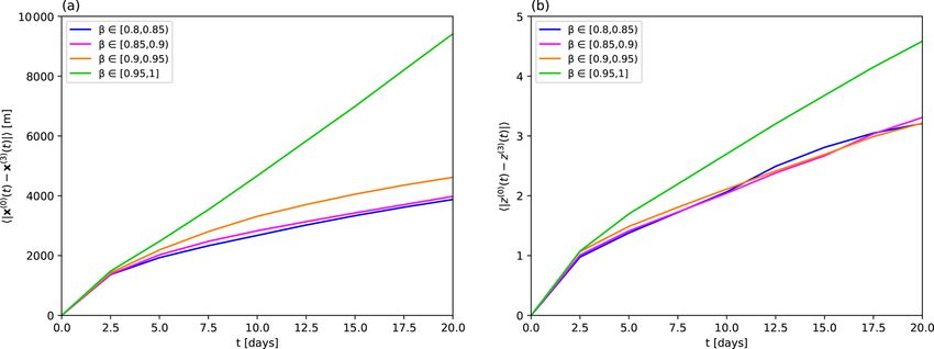
We illustrate the impact of this variable density on particle atively buoyant and of which 6 % originates from maritime
trajectories for the summer release in Fig. 4. Here we com- activities) to compute the rate r at which microplastic parti-
pute, as a function of time, the range of horizontal |x(0) −x(1) | cles of our interest enter the water column in the open sea:
and vertical |z(0) − z(1) | distances and its average among r = 4000 t/year ×0.37 × 0.06 = 88.8 t/year, or r = 0.24 t/d.
particles. Trajectories x (0) (t) and x (1) (t) are obtained with The next step is to estimate the time during which these
constant nominal fluid density (1025 kg/m3 ) and position- microplastic particles remain in the water column before
dependent fluid density, respectively, using the same release reaching the sea bottom. We take the mean depth for the
location and date, 8 July 2000, in both cases. Particle density Mediterranean to be h = 1480 m (Eakins and Sharman,
is fixed at ρp = 1041.5 kg/m3 . The difference between the 2010; GEBCO Compilation Group, 2020) and estimate a res-
two calculations (and thus the error of considering that con- idence time τ as the time of sinking to that mean depth. The
stant value for the density) should be compared to average residence time depends on the sinking velocity, τ = h/vs ,
horizontal and vertical displacements of 95 km and 124 m, and thus on the physical properties of the microplastic par-
respectively, at t = 20 d. At that time, we thus find that the ticles. Assuming a seawater density ρf = 1025 kg/m3 , and
influence of variable fluid density on the dynamics is about the range of plastic densities and their proportions described
3 % for the horizontal movement and 6 % for the vertical dis- in Sect. 3.1, we see from Eq. (2) that for microplastic parti-
placement on average. cles of radius a ≈ 0.05 mm the range of sinking velocities is
A summary of the average relative differences on horizon- 6.20–509.23 m/d, giving a residence time in the range 3.1–
tal and vertical particle positions between using the location- 255 d. Averaging these times weighted by the proportion of
dependent seawater density and a nominal constant value each type of plastic we get τ ≈ 14 d. Combining the input
ρf = 1025 kg/m3 , both in winter and summer periods, is dis- rate r with this mean residence time we get an estimate for
played in Table 1. The relative error produced by assuming the total amount present in the water column at any given
a constant density is larger in the vertical direction. It is also time as Q = rτ : the result is Q ≈ 3.36 t of dense rigid mi-
larger for the release in winter, but this is a consequence of croplastics if all of them would be in the form of particles of
taking a value for the reference density that is not representa- size a = 0.05 mm. This is below but close to 1 % of the esti-
tive of winter waters but is strongly biased (see Fig. 3, right). mated upper bound of 470 t of floating plastic in the Mediter-
If using a reference value more appropriate for winter waters ranean (according to the corresponding estimation of Kaan-
(say ρf ≈ 1027 kg/m3 ) the relative error remains quite small, dorp et al., 2020).
due to the weaker stratification of the sea during this season. We emphasize the many uncertainties affecting this result
In fact, the reference value is also biased in the summer un- (Sect. 3.1 and 3.2), and we highlight the one related to parti-
less the investigation is restricted to the surface. cle size: because of the quadratic dependence of the sinking
In brief, we see that the effect of location-dependent den- velocity on the particle radius a, Eq. (2), choosing the par-
sity may be a relevant effect to evaluate microplastic trans- ticle size to be half of the one used here will lead to an es-
port. At least, the traditional value of seawater density may timate 4 times larger for the mass if the same release rate is
be biased, which may be reflected in the particle trajectories. assumed. This enhanced retention of smaller particles in the
We recall, however, that we used parameters for the particle water column may imply, depending on the actual size dis-
properties for which they are slowly falling. The impact of tribution, a dominance of very small particles on the plastic
https://doi.org/10.5194/os-17-431-2021 Ocean Sci., 17, 431–453, 2021438 R. de la Fuente et al.: Sinking microplastics in the water column Figure 3. Normalized histogram of the seawater density ρf at the positions of N = 78 803 particles after t = 0, 10, and 20 d of being released over the whole Mediterranean. (a) Summer release (release date 8 July 2000). (b) Winter release (release date 8 January 2000). The particles’ density is fixed at ρp = 1041.5 kg/m3 , and fluid density is obtained from the TEOS-10 equations. The vertical line indicates a conventional seawater density of 1025 kg/m3 . Figure 4. The distance, as a function of time, between trajectories obtained with constant nominal fluid density of ρf = 1025 kg/m3 and the actual variable fluid density, both starting at the same initial location. The range of the values among all particles released in different points of the Mediterranean is indicated by the shaded area, while the solid line indicates the average over the particles. Particles have ρp = 1041.5 kg/m3 , and all parameters are the same as for the summer release in Fig. 3. (a) Horizontal distances. (b) Vertical distances. mass content of the water column. However, our estimates of turbulence might cause an increase in lifetimes of particles plastic input into the ocean (we use mainly Kaandorp et al., in the water column, dense water formation and rapid con- 2020) rely on observations that do not catch extremely small vection, a process reported in areas such as the Gulf of Lion, particles. These considerations further justify our choice of a would likely reduce particle retention time. These events take radius a = 0.05 mm, small but still easily detectable, as con- place in winter and were shown to transfer particles from venient to provide reasonable estimations of negatively buoy- the ocean surface to mid-waters (1000 m) and deep ocean ant rigid microplastic mass in the water column within com- (> 2000 m) in a very short time (1–2 d) and lead to the forma- monly quoted size ranges. We can not exclude larger plastic tion of bottom nepheloid layers (de Madron et al., 1999; Vi- content at smaller sizes. Another source of bias may be that dal et al., 2009; Heussner et al., 2006; Stabholz et al., 2013). in this study the impact of small-scale turbulence and con- The result for the total mass is independent of the hori- vective mixing events is not considered. While small-scale zontal distribution of particle release, which is quite inho- Ocean Sci., 17, 431–453, 2021 https://doi.org/10.5194/os-17-431-2021
R. de la Fuente et al.: Sinking microplastics in the water column                                                                   439

mogeneous (Fig. 1 of Liubartseva et al., 2018). However,
for a rough estimate of the density of these microplastics in
the water column, we assume a uniform particle distribution
over the whole Mediterranean both in the horizontal and in
the vertical. Since the volume of the Mediterranean is about
4.39 × 10⁶ km3 (Eakins and Sharman, 2010) the estimated
density would be ρV ≈ 7.7 × 10⁻¹¹ kg/m3 (with the above-
discussed scaling issues with a). We remind the reader that
this is a value for the open sea, and our study does not address
coastal areas, where the density would likely be higher.
   The above estimates are rather rough as a result of the un-
certainties mentioned. The assumption of a uniform distribu-
tion in the vertical direction has not yet been justified either,
but we will show it to be appropriate by means of our simula-
tions of particle release starting at 1 m depth over the whole
Mediterranean. Instead of performing a continuous release           Figure 5. The continuous line is the area that the Mediterranean
of new particles at each time step, and computing statistics        has at each depth z. The dashed line is microplastic density per unit
over this growing number of sinking particles, we approxi-          of depth ρ(z) under continuous release of particles with β = 0.8
mate this by the statistics of all positions at all time steps of   at 1 m depth. Both curves have been normalized to have unit area,
a set of particles deployed in a single release event. This as-     so that they can be compared on the same scale. The binning size
sumes a time-independent fluid flow, but this approximation         is 100 m. The inset shows the ratio ρ(z)/A(z), proportional to the
is appropriate, since the dispersion of an ensemble of par-         mass density of microplastic per unit of volume ρV (z).
ticles released in a single event follows rather well-defined
statistical laws (see Sect. 4.4) and is thus independent of the
time-varying details of the flow. Particles are removed when
                                                                    tion u is negligible, at least when considering its effect over
touching the bottom. For our estimate, we use β = 0.8, i.e.,
                                                                    the whole Mediterranean. Another possibility is that the fluc-
assuming the fastest sinking velocity of typical plastic parti-
                                                                    tuating flow component u in Eq. (1) results in a vertical dis-
cles, for which particles reach vertical depths deeper if com-
                                                                    persion compatible with a constant concentration. Although
pared with the slower sinking velocities used in our study.
                                                                    the former explanation predicts an alteration from a constant
   Figure 5 shows ρ(z), the density of plastic particles per
                                                                    if the settling velocity is sufficiently small to allow u to in-
unit of depth z in the whole Mediterranean, and also A(z),
                                                                    duce a stronger vertical dispersion, we will see in the next
the amount of area that the Mediterranean has at each depth
                                                                    section that a nearly constant concentration may be assumed
z. Both functions have been normalized such that the value
                                                                    for the majority of our parameter range.
of their integrals with respect to z is one; in this way the
functions can be displayed in the same plot. We see that
both curves are nearly identical (in fact, just proportional,       4.4   Transient evolution
because of the normalization), indicating that the variation
of the number of particles with depth is essentially due to the     We now analyze in detail the transient evolution of parti-
decrease in sea area with depth. A clearer way to see that is       cle clouds initialized by flash releases at a fixed depth. Nu-
to plot ρ(z)/A(z), which is proportional to the mean plas-          merically we proceed by releasing N = 78 803 particles uni-
tic concentration per unit volume at each depth z, ρV (z). We       formly distributed over the entire Mediterranean surface at
see that this quantity is nearly constant, at least in the first    1 m depth in the winter season, as already described. They
3000 m. At larger depths a weak increase seems to occur, but        evolve according to Eq. (1) using a constant water density.
this is made unclear by the poor statistics arising from the        We take three examples for the particle density, which corre-
small area and number of particles present at these depths.         spond to β = 0.8, 0.9 and 0.99, or vs = 153.48, 68.21 and
Thus, the hypothesis of a uniform distribution of plastic in        6.20 m/d for our particles of radius a = 0.05 mm, respec-
the water column seems to be a reasonable description of the        tively; in what follows, these setups shall be denominated as
simulation of the fastest-sinking particles.                        v153, v68 and v6. The horizontal displacements during the
   A uniform distribution of plastics in z is what is expected if   particle sinking times are much larger (of the order of 60 km)
the vertical velocity of the particles is exactly constant (since   than the sea depth, so that in fact the particles are sinking
each particle will spend exactly the same amount of time at         sideways (Siegel and Deuser, 1997). However, the horizontal
each depth interval). The equation of motion used (Eq. 1) cor-      displacements still remain very small compared to the basin
rects this constant sinking velocity v s with a contribution u      size, and we concentrate on the vertical motion. Even though
from the ambient flow. Thus, the close-to-constant character        the vertical steady distribution has been found to be close to
of the plastic concentration may imply that the flow correc-        uniform in Sect. 4.3, the reason for this is not evident, and

https://doi.org/10.5194/os-17-431-2021                                                               Ocean Sci., 17, 431–453, 2021
440 R. de la Fuente et al.: Sinking microplastics in the water column
we will give support here for the pertinence of this finding to
most of the relevant parameter range.
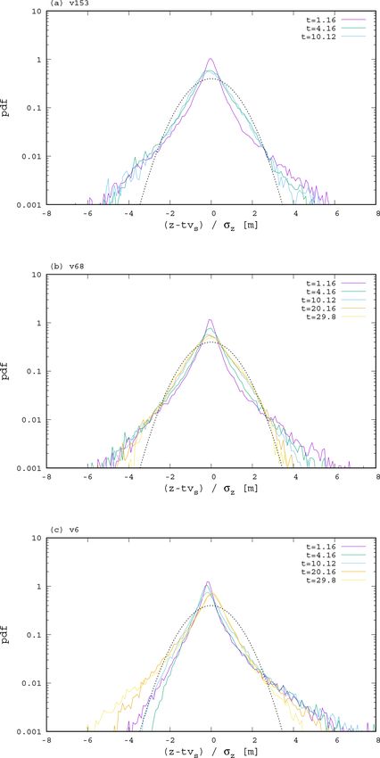
Figure 6 shows the vertical particle distribution at differ-
ent times (upper plot is for v153, middle for v68 and bot-
tom for v6). The plot is given in terms of a rescaled variable
z̃ = z−tv s 2 2
σz where σz ≡ h(zi −hzi i) i is the variance of the par-
ticles’ z coordinate. Here the subindex i refers to the parti-
cle and h. . .i denotes averaging over different particles. Thus,
we plot in the figure the rescaled distribution of the parti-
cles around the average depth of the particles at any given
time. For comparison, the normal distribution is plotted with
dashed lines. This figure shows deviations from Gaussianity
for early times. The deviation from normal distribution de-
creases for later instants but remains considerable, especially
for the tails, which may also be indicative of anomalous
diffusive behavior. For reference, particles reach the mean
Mediterranean depth, h = 1480 m, at times τ = 9.64, 21.8
and 246.7 d for v153, v68 and v6, respectively.
Since a non-Gaussian distribution is usually linked
to anomalous dispersion (Neufeld and Hernández-García,
2009), we now analyze this aspect in detail by considering
how the variance of the vertical particle distribution, σz2 (t),
evolves. Although there is a continual loss of particles be-
cause of reaching the seafloor with a varied topography, we
illustrate in Appendix C that our conclusions are likely unaf-
fected by this effect.
According to Fig. 7, dispersion appears to be governed
by different laws in different regimes, which we shall dis-
tinguish by the approximate effective exponents ν, defined
through approximate behaviors σz2 ∼ t ν in different time in-
tervals.
We start our analysis with the fastest-sinking particles
(v153; Fig. 7a). At the very beginning, superdiffusion takes
place with ν > 2, which may be related to autocorrelation in
the flow, but we will iterate on this question when compar-
ing different settling velocities. Around t = 1 d, the evolution
seems to become consistent with normal diffusion (ν = 1),
usual after initial transients in oceanic turbulence (Berloff
and McWilliams, 2002; Reynolds, 2002). However, around
t = 4.5 d, we can observe a crossover to ballistic dispersion
(ν = 2). Figure 6. The probability density function, estimated from a his-
We explain this last crossover as resulting from a differ- togram of bin size 0.1, of all particles released in the Mediterranean
ent mean sinking velocity in diverse regions of the Mediter- in the rescaled variable z̃ = z−tv s
σz for the different setups (v153,
ranean, associated with up- and down-welling. This can be v68 and v6) and times (in days) as indicated. For comparison, nor-
modeled in an effective way by writing the vertical position mal distributions of zero mean and unit variance are shown with a
of particle i as dashed line.
zi = hzi i + ω̄i t + Wi , (5) coefficient Di for each trajectory by Wi2 = Di t. The overbar
refers to temporal averaging for asymptotically long times
where h. . .i denotes, as before, an averaging over different along the trajectory of a given particle (but assuming that the
particles. Here we are assuming that zi −hzi i evolves accord- particle remains in a region with a well-defined ω̄i 6= 0), and
ing to the sum of a constant average velocity contribution ω̄i Di characterizes the strength of the fluctuations. Assuming
for sufficiently long times (a characteristic of the flow region hω̄i Wi i = 0,
traversed by particle i), and of Wi , a Wiener process repre-
senting fluctuations with zero mean and defining a diffusion σz2 ≡ h(zi − hzi i)2 i = hω̄i2 it 2 + hDi it, (6)
Ocean Sci., 17, 431–453, 2021 https://doi.org/10.5194/os-17-431-2021R. de la Fuente et al.: Sinking microplastics in the water column 441
Figure 8. ω̄i as estimated from t = 10.83 d plotted at the initial po-
sition of each particle i in the v153 simulation. The black rectangle
in the Western Mediterranean is the area of large depth considered
in Appendix C.
tions should already have become negligible. The horizon-
tal pattern of the estimated ω̄i is presented in Fig. 8, which
confirms its patchiness throughout the Mediterranean, asso-
ciated with mesoscale features. Computing hω̄i2 i and fitting a
line to σz2 (t) between t = 1.4 and 4 d to estimate D, we ob-
tain t ∗ ≈ 4.5 d from Eq. (7), which remarkably agrees with
Fig. 7a. After approximately t = 12 d there is hardly any dis-
persion, since most of the particles are close to the sea bottom
(cf. Fig. 9) where the vertical fluid velocity is nearly zero.
Note also a small drop in σz2 at the very end of the time se-
ries, where the results may actually be subject to artifacts; see
Appendix C. However, this is of minor importance, since the
distribution of particles so close to the bottom should never-
theless be strongly influenced by resuspension and remixing
by bottom currents (Kane et al., 2020).
The different regimes are not as clear in the v68 case as for
v153; see Fig. 7b. One evident novel feature is a subdiffusive
regime during the transient from the initial superdiffusion
(as in the case of horizontal tracer dispersion in the ocean
studied by Berloff and McWilliams (2002) and Reynolds
(2002)). Approximate normal diffusion is then observed until
Figure 7. Variance of depth reached by the particles as a function
t = 10 d, when a crossover to a faster dispersion does seem
of time. Straight lines represent power laws for reference, with ex- to take place; see the inset. A fit of normal diffusion from
ponents 1 (in green, corresponding to standard diffusion) and 2 (in t = 4 to 8 d and the velocity variance at t = 12.5 d give an
purple, corresponding to ballistic dispersion). estimate t ∗ ≈ 11.7. However, the long-term ballistic regime
is not clear. In fact, a long-term return from such a ballistic
regime to normal diffusion is expected as a result of increas-
that is, the variance is a sum of a ballistic and a normal dif- ing horizontal mixing, which renders ω̄i time dependent and
fusive term, associated with regional differences in the mean makes it approach zero. According to a careful visual inspec-
velocity and with fluctuations, and dominating for long and tion of the inset in Fig. 7b, this may take place already around
short times, respectively. Writing D = hDi i, the crossover t = 14 d.
between the two regimes is obtained by equating the two For v6 (Fig. 7c), the transition from the initial superdiffu-
terms as sive regime to that of normal diffusion appears to not involve
D subdiffusion. This is already informative: the fluid velocity
t∗ = . (7) field is the same for the three simulations with different set-
hω̄i2 i
tling velocity, so the differences must originate from the dif-
To evaluate Eq. (7), we first estimate ω̄i for each par- ferent rates of sampling of the different fluid layers by parti-
ticle from the “asymptotically” long time of t = 10.83 d, cles while they sink. In particular, the decay of autocorrela-
which is the latest time after the crossover still in the bal- tion is obviously faster for faster-sinking particles, since it is
listic regime in Fig. 7a, when the contribution of fluctua- determined by the spatial structure of the velocity field.
https://doi.org/10.5194/os-17-431-2021 Ocean Sci., 17, 431–453, 2021442 R. de la Fuente et al.: Sinking microplastics in the water column
scale nature is input to the equation (such that small-scale
turbulence is not resolved), or when the variability in seawa-
ter density is neglected, moderate but possibly non-negligible
errors emerge (Nooteboom et al., 2020). However, our con-
clusions about the vertical distribution and dispersion of mi-
croplastics rely on robust features of the large-scale flow and
must remain unaffected by moderate errors. We also note that
the traditional value of seawater density, ρf = 1025 kg/m3 ,
is representative only for near-surface layers in the summer,
and correcting for the bias could reduce the error of simula-
tions with a constant seawater density. A suitable equation of
motion for the particles considered is constructed by adding
Figure 9. Variance of depth reached by the particles as a function to the external velocity field a constant settling term, as also
of their mean depth. found by Monroy et al. (2017) for marine biogenic particles.
When the velocity field of the Mediterranean Sea is ap-
proximated by realistic simulation, this equation of motion
While this is one possible explanation for the earlier tim- results in a nearly uniform steady distribution along the wa-
ing of the initial transition from anomalous to normal diffu- ter column, except perhaps at extremely low settling veloci-
sion for higher settling velocity, one cannot exclude that a ties. The corresponding total amount of plastic present in the
depth-dependent organization of the flow is more in play; water column is relatively small, close to 1 % of the float-
note that ν > 2 at the beginning, which might not be ex- ing plastic mass, but it may be an important contribution to
plained by simple autocorrelation but might be characteristic the microplastic pollution in deep layers of the ocean and is
of properties of the velocity field at those depths. The gov- subject to several uncertainties.
erning role of the spatial structure is supported by Fig. 9: the Note that only those microplastic particles are considered
transition in question takes place at the same depth (≈ 100 m) here that have not yet sedimented on the bottom, and the plas-
in the different simulations, which seems to point to mixed- tic amount sedimented on the seafloor is large (Fischer et al.,
layer processes. Depth dependence might also govern the 2015; Liubartseva et al., 2018; Peng et al., 2018; Mountford
suppression of ballistic dispersion for long times, but it is and Morales Maqueda, 2019; Soto-Navarro et al., 2020). The
very unclear. suitability of our equation of motion to describe the sink-
Note in Fig. 9 that the vertical variance is not expected to ing of a class of microplastic particles implies that advec-
grow much larger for v68 than for v153 even if the simulation tion by the flow may contribute to large-scale horizontal in-
were longer. Therefore, even if the constancy of the steady homogeneity of deep-sea plastic sediments by means of re-
vertical distribution relies on the weak vertical dispersion for cently described noninertial mechanisms (Drótos et al., 2019;
v153 (see Sect. 4.3), constancy is expected to hold in most Monroy et al., 2019; Sozza et al., 2020). This may be espe-
of our parameter range. A considerably stronger dispersion cially so in regions where redistribution by bottom flows is
and a possible corresponding deviation from constancy may restricted to small distances, like abyssal plains (Kane and
arise only for extremely low settling velocities, like for v6 in Clare, 2019). Resuspension and redistribution may be domi-
Fig. 9. nant in forming sedimented patterns (Kane et al., 2020), and
a future investigation should take all processes into account
to identify zones of high plastic concentration on the sea bot-
5 Conclusions tom.
As for the vertical distribution profile, its approximate uni-
We have discussed the different types of plastics occurring in formity may be linked to the weak vertical dispersion of par-
the water column, pointing out gaps in our knowledge about ticles that is found in our simulations, started with a flash
the sources, transport pathways and properties of such par- release over the whole surface of the Mediterranean sea. The
ticles. It would be highly beneficial to have distributions of shape of the emerging transient vertical distribution exhibits
size, polymer type and quantifiers of shape recorded sepa- deviations from a Gaussian, which are related to anomalous
rately for the dynamically different classes of microplastics. diffusive laws that dominate the vertical dispersion process
We have focused our attention on rigid microplastic par- in some phases.
ticles with negative buoyancy. We have argued that the sim- The different diffusive laws are related to the properties
plified MRG equation approximates the dynamics of such of the decay in the Lagrangian velocity autocorrelation de-
particles sufficiently well for qualitative estimations. fined along the trajectories of the sinking particles. An impor-
We have then analyzed the importance of different effects tant example is the transition from initial superdiffusion to a
in this equation and concluded that the Coriolis and the in- longer phase of normal diffusion, occurring around 100 m
ertial terms are negligible. When a velocity field of large- depth, which indicates that the particles enter into a different
Ocean Sci., 17, 431–453, 2021 https://doi.org/10.5194/os-17-431-2021You can also read