Development and application of a United States-wide correction for PM2.5 data collected with the PurpleAir sensor - Recent
←
→
Page content transcription
If your browser does not render page correctly, please read the page content below

Atmos. Meas. Tech., 14, 4617–4637, 2021
https://doi.org/10.5194/amt-14-4617-2021
© Author(s) 2021. This work is distributed under
the Creative Commons Attribution 4.0 License.

Development and application of a United States-wide correction for
PM2.5 data collected with the PurpleAir sensor
Karoline K. Barkjohn1 , Brett Gantt2 , and Andrea L. Clements1
1 Office of Research and Development, US Environmental Protection Agency, 109 T.W. Alexander Drive,
Research Triangle Park, NC 27711, USA
2 Office of Air Quality Planning and Standards, US Environmental Protection Agency, 109 T.W. Alexander Drive,

Research Triangle Park, NC 27711, USA

Correspondence: Karoline K. Barkjohn (barkjohn.karoline@epa.gov)

Received: 16 October 2020 – Discussion started: 2 December 2020
Revised: 27 April 2021 – Accepted: 29 April 2021 – Published: 22 June 2021

Abstract. PurpleAir sensors, which measure particulate mat-      tion, along with proposed data cleaning criteria, has been ap-
ter (PM), are widely used by individuals, community groups,      plied to PurpleAir PM2.5 measurements across the US on the
and other organizations including state and local air monitor-   AirNow Fire and Smoke Map (https://fire.airnow.gov/, last
ing agencies. PurpleAir sensors comprise a massive global        access: 14 May 2021) and has the potential to be success-
network of more than 10 000 sensors. Previous performance        fully used in other air quality and public health applications.
evaluations have typically studied a limited number of Pur-
pleAir sensors in small geographic areas or laboratory envi-
ronments. While useful for determining sensor behavior and
data normalization for these geographic areas, little work has   1   Introduction
been done to understand the broad applicability of these re-
sults outside these regions and conditions. Here, PurpleAir      Fine particulate matter (PM2.5 , the mass of particles with
sensors operated by air quality monitoring agencies are eval-    aerodynamic diameters smaller than 2.5 µm) is associated
uated in comparison to collocated ambient air quality regula-    with a number of negative health effects (Schwartz et al.,
tory instruments. In total, almost 12 000 24 h averaged PM2.5    1996; Pope et al., 2002; Brook et al., 2010). Short-term and
measurements from collocated PurpleAir sensors and Fed-          long-term exposures to PM2.5 are associated with increased
eral Reference Method (FRM) or Federal Equivalent Method         mortality (Dominici et al., 2007; Franklin et al., 2007; Di
(FEM) PM2.5 measurements were collected across diverse           et al., 2017). Even at low PM2.5 concentrations, significant
regions of the United States (US), including 16 states. Con-     health impacts can be seen (Bell et al., 2007; Apte et al.,
sistent with previous evaluations, under typical ambient and     2015), and small increases of only 1–10 µg m−3 can increase
smoke-impacted conditions, the raw data from PurpleAir           negative health consequences (Di et al., 2017; Bell et al.,
sensors overestimate PM2.5 concentrations by about 40 %          2007; Grande et al., 2020). In addition to health effects,
in most parts of the US. A simple linear regression reduces      PM2.5 can harm the environment, reduce visibility, and dam-
much of this bias across most US regions, but adding a rel-      age materials and structures (Al-Thani et al., 2018; Ford et
ative humidity term further reduces the bias and improves        al., 2018). Understanding PM2.5 at fine spatial and temporal
consistency in the biases between different regions. More        resolutions can help mitigate risks to human health and the
complex multiplicative models did not substantially improve      environment, but the high cost and complexity of conven-
results when tested on an independent dataset. The final Pur-    tional monitoring networks can limit network density (Sny-
pleAir correction reduces the root mean square error (RMSE)      der et al., 2013; Morawska et al., 2018).
of the raw data from 8 to 3 µg m−3 , with an average FRM            Lower-cost air sensor data may provide a way to better
or FEM concentration of 9 µg m−3 . This correction equa-         understand fine-scale air pollution and protect human health.
                                                                 Air sensors are widely used by a broad spectrum of groups,

Published by Copernicus Publications on behalf of the European Geosciences Union.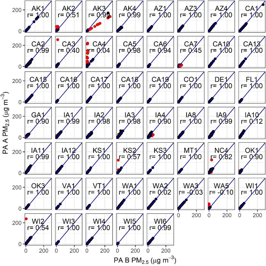
4618              K. K. Barkjohn et al.: Development and application of a United States-wide correction for PM2.5 data

from air quality monitoring agencies to individuals. Sensors       Kuula et al., 2020a; Ford et al., 2019; Si et al., 2020; Zou
offer the ability to measure air pollutants at higher spatial      et al., 2020b; Tryner et al., 2020b). Although not true of all
and temporal scales than conventional monitoring networks          types of PM2.5 sensors, previous work with PurpleAir sen-
with potentially less specialized operating knowledge and          sors and other models of Plantower sensors has shown that
cost. However, concerns remain about air sensor data qual-         the sensors are precise, with sensors of the same model mea-
ity (Clements et al., 2019; Williams et al., 2019). Typically,     suring similar PM2.5 concentrations (Barkjohn et al., 2020;
air sensors require correction to become more accurate com-        Pawar and Sinha, 2020; Malings et al., 2020). However, ex-
pared to regulatory monitors. A best practice is to locate air     tensive work with PurpleAir and Plantower sensors has of-
sensors alongside regulatory air monitors to understand their      ten shown deficiencies in the accuracy of the measurement,
local performance and to develop corrections for each indi-        resulting in the need for correction. A number of previous
vidual sensor (Jiao et al., 2016; Johnson et al., 2018; Zusman     corrections have been developed; however, they are typically
et al., 2020). For optical particulate matter (PM) sensors, cor-   generated for a specific region, season, or condition, and lit-
rection procedures are often needed due to both the chang-         tle work has been done to understand how broadly applicable
ing optical properties of aerosols associated with both their      they are (Ardon-Dryer et al., 2020; Magi et al., 2019; Delp
physical and chemical characteristics (Levy Zamora et al.,         and Singer, 2020; Holder et al., 2020; Tryner et al., 2020a;
2019; Tryner et al., 2019) and the influence of meteorolog-        Robinson, 2020). Although location-specific and individual
ical conditions including temperature and relative humidity        sensor corrections may be ideal, the high precision suggests
(RH) (Jayaratne et al., 2018; Zheng et al., 2018). In addition,    that a single correction across PurpleAir sensors may be pos-
some air sensors have out-of-the box differences and low pre-      sible. This is especially important since having multiple cor-
cision between sensors of the same model (Feenstra et al.,         rections can make it difficult for many sensor users to know
2019; Feinberg et al., 2018). Although collocation and local       which correction is best for their application.
correction may be achievable for researchers and some air             In this work, we develop a US-wide correction for Pur-
monitoring agencies, it is unattainable for many sensor users      pleAir data which increases accuracy across multiple re-
and community groups due to lack of access and proximity           gions, making it accurate enough to communicate the air
to regulatory monitoring sites.                                    quality index (AQI) to support public health messaging. We
   PurpleAir sensors are a PM sensor package consisting of         use onboard measurements and information that would be
two laser scattering particle sensors (Plantower PMS5003),         available for all PurpleAir sensors, even those in remote ar-
a pressure–temperature–humidity sensor (Bosch BME280),             eas far from other monitoring or meteorological sites.
and a WiFi-enabled processor that allows the data to be up-
loaded to the cloud and utilized in real time. The low cost of
outdoor PurpleAir sensors (USD 230–260) has enabled them           2     Data collection
to be widely used with thousands of sensors publicly report-
ing across the US. Previous work has explored the perfor-          2.1    Site identification
mance and accuracy of PurpleAir sensors under outdoor am-
bient conditions in a variety of locations across the United       Data for this project came from three sources: (1) PurpleAir
States including in Colorado (Ardon-Dryer et al., 2020;            sensors sent out by the EPA for collocation to capture a wide
Tryner et al., 2020a); Utah (Ardon-Dryer et al., 2020; Kelly       range of regions and meteorological conditions; (2) privately
et al., 2017; Sayahi et al., 2019); Pennsylvania (Malings et       operated sensor data volunteered by state, local, and tribal
al., 2020); North Carolina (Magi et al., 2019); and in Califor-    (SLT) air monitoring agencies independently operating col-
nia, where the most work has occurred to date (Ardon-Dryer         located PurpleAir sensors; and (3) publicly available sensors
et al., 2020; Bi et al., 2020; Feenstra et al., 2019; Mehadi       located near monitoring stations and confirmed as true col-
et al., 2020; Schulte et al., 2020; Lu et al., 2021). Their        location by air monitoring agency staff. In order to identify
performance has been explored in a number of other parts           publicly available collocated sensors, in August of 2018, a
of the world as well including in Korea (Kim et al., 2019),        survey of sites with potentially collocated PurpleAir sensors
Greece (Stavroulas et al., 2020), Uganda (McFarlane et al.,        and regulatory PM2.5 monitors was performed by identify-
2021), and Australia (Robinson, 2020). Additional work has         ing publicly available PurpleAir sensor locations within 50 m
been done to evaluate their performance under wildland-fire-       of an active EPA Air Quality System (AQS) site reporting
smoke-impacted conditions (Bi et al., 2020; Delp and Singer,       PM2.5 data in 2017 or 2018. The 50 m distance was selected
2020; Holder et al., 2020), indoors (Z. Wang et al., 2020),        because it is large enough to cover the footprint of most AQS
and during laboratory evaluations (Kelly et al., 2017; Kim et      sites and small enough to exclude most PurpleAir sensors in
al., 2019; Li et al., 2020; Mehadi et al., 2020; Tryner et al.,    close proximity of but not collocated with an AQS site. From
2020a; Zou et al., 2020a, b). The performance of their dual        a download of all active AQS PM2.5 sites and PurpleAir sen-
Plantower PMS5003 laser scattering particle sensors has also       sor locations on 20 August 2018, 42 unique sites were iden-
been explored in a variety of other commercial and custom-         tified in 14 states (data from additional states were available
built sensor packages (He et al., 2020; Tryner et al., 2019;       from sensors sent out by the EPA and privately operated sen-

Atmos. Meas. Tech., 14, 4617–4637, 2021                                              https://doi.org/10.5194/amt-14-4617-2021
K. K. Barkjohn et al.: Development and application of a United States-wide correction for PM2.5 data                           4619

sors). From this list of public PurpleAir sensors potentially       24 h PM2.5 averages occurred less frequently, they may have
collocated with regulatory PM2.5 monitors, we reached out           larger public health consequences and be of greater interest
to the appropriate SLT air monitoring agency to understand          to communities. To preserve more of the high-concentration
if these units were operated by the air monitoring agency and       data, the Iowa PurpleAir PM2.5 data were split into 10 bins
their interest in partnering in this research effort. If we could   from 0–64 µg m−3 by 6.4 µg m−3 increments. Since there
not identify the sensor operator of these 42 sensors or if the      were fewer data in the higher-concentration bins, all data in
sensor was not collocated at the air monitoring station, the        bins 6–10 (≥ 25 µg m−3 ) were included, and an equal num-
sensor was not used in this analysis.                               ber of randomly selected data points was selected from each
    Much past work using public data from PurpleAir has used        of the other four bins (N = 649). The subset and full com-
public sensors that appear close to a regulatory station on the     plement of Iowa data were compared visually, and the dis-
map (Ardon-Dryer et al., 2020; Bi et al., 2020). However,           tributions of the temperature and RH for both datasets were
there is uncertainty in the reported location of PurpleAir sen-     similar (Fig. S1), with a similar range of dates represented
sors as this is specified by the sensor owner. In some cases,       from September 2017 until January of 2020.
sensors may have the wrong location. Known examples in-
clude owners who forgot to update the location when they            2.2     Air monitoring instruments and data retrieval
moved, take the sensor inside for periods to check their in-
door air quality, or specifically choose an incorrect location      2.2.1    PurpleAir sensors
to protect their privacy. In addition, without information on
local sources of PM2.5 , it can be unclear how far away is ac-      The PurpleAir sensor contains two Plantower PMS5003 sen-
ceptable for a “collocation” since areas with more localized        sors, labeled as channel A and B, that operate for alternat-
sources will need to be closer to the reference monitor to          ing 10 s intervals and provide 2 min averaged data (prior to
experience similar PM2.5 conditions. By limiting this work          30 May 2019, this was 80 s averaged data). Plantower sensors
to true collocations operated by air monitoring agencies, we        measure 90◦ light scattering with a laser using 680 ± 10 nm
eliminate one source of uncertainty. We can conclude that the       wavelength light (Sayahi et al., 2019) and are factory cali-
PurpleAir errors measured in this work are not due to poor          brated using ambient aerosol across several cities in China
siting or localized sources and can focus on other variables        (Malings et al., 2020). The Plantower sensor reports esti-
that influence error (e.g., RH).                                    mated mass of particles with aerodynamic diameters < 1 µm
    When the EPA provided PurpleAir sensors to air monitor-         (PM1 ), < 2.5 µm PM2.5 , and < 10 µm (PM10 ). These values
ing agencies, the EPA suggested that they be deployed with          are reported in two ways, labeled as cf_1 and cf_atm, in the
similar siting criteria as regulatory monitors. Some sites had      PurpleAir dataset, which match the “raw” Plantower outputs.
space and power limitations to consider, but trained techni-        PurpleAir previously had these cf_1 and cf_atm column la-
cians sited sensors allowing adequate unobstructed airflow.         bels flipped in the data downloads (Tryner et al., 2020a),
In many cases, sensors were attached to the top rung of the         but for this work we have used the updated labels. The two
railings at the monitoring shelters, where they were within a       data columns have a [cf_atm] / [cf_1] = 1 relationship below
meter or so of other inlet heights and within 3 m or so of the      roughly 25 µg m−3 (as reported by the sensor) and then tran-
other instrument inlets.                                            sition to a two-thirds ratio at higher concentration ([cf_1]
    In total, 53 PurpleAir sensors at 39 unique sites across 16     concentrations are higher). The cf_atm data, displayed on the
states were ideal candidates and were initially included in         PurpleAir map, are the lower measurement of PM2.5 and will
this analysis with data included from September 2017 until          be referred to as the “raw” data in this paper when making
January 2020. The Supplement contains additional informa-           comparison between initial and corrected datasets. In addi-
tion about each AQS site (Table S1) and each individual sen-        tion to PM2.5 concentration data, the PurpleAir sensors also
sor (Table S2).                                                     provide the count of particles per 0.1 liter of air above a spec-
                                                                    ified size in micrometers (i.e., > 0.3, > 0.5, > 1.0, > 2.5,
Subsetting the Iowa dataset                                         > 5.0, > 10 µm); however, these are actually calculated re-
                                                                    sults as opposed to actual size bin measurements (He et al.,
Initially, there were 10 907 pairs of 24 h averaged collo-          2020).
cated data from Iowa, which was 55 % of the entire collo-              When a PurpleAir sensor is connected to the internet, data
cated dataset. In order to better balance the dataset among         are sent to PurpleAir’s data repository on ThingSpeak. Users
the states and to avoid building a correction model that is         can choose to make their data publicly viewable (public) or
weighted too heavily towards the aerosol and meteorologi-           control data sharing (private). Agencies with privately re-
cal conditions experienced in Iowa, the number of days from         porting sensors provided application programming interface
Iowa was reduced to equal the size of the California dataset,       (API) keys so that data could be downloaded. PurpleAir PA-
the state with the next largest quantity of data (29 % of the       II-SD models can also record data offline on a microSD card;
entire collocated dataset). When reducing the Iowa dataset,         however, these offline data appeared to have time stamp er-
the high-concentration data were preserved. Although high           rors from internal clocks that drift without access to the fre-

https://doi.org/10.5194/amt-14-4617-2021                                              Atmos. Meas. Tech., 14, 4617–4637, 2021
4620              K. K. Barkjohn et al.: Development and application of a United States-wide correction for PM2.5 data

quent time syncs available with access to WiFi, so they were     surements was evaluated using the FRM performance as-
excluded from this project. Data were downloaded from the        sessments (U.S. EPA, 2020b). They were evaluated using
ThingSpeak API using Microsoft PowerShell at the native          the FRM–FRM precision and bias, the average field blank
2 min or 80 s time resolution and were saved as csv files        weight, and the monthly precision. The performance of the
that were processed and analyzed in R (R Development Core        FEM monitors was evaluated using the PM2.5 continuous
Team, 2019).                                                     monitor comparability assessments (U.S. EPA, 2020a). FEM
                                                                 measurements are compared to simultaneous Federal Ref-
2.2.2    Federal Reference Method (FRM) and Federal              erence Method (FRM) measurements. Linear regression is
         Equivalent Method (FEM) PM2.5                           used to calculate a slope, intercept (int), and correlation (R),
                                                                 and the FEM / FRM ratio is also computed. Based on data
On 20 February 2020, 24 h averaged PM2.5 reference data          quality objectives, the slope should be between 0.9 and 1.1,
were downloaded for the 39 collocation sites from the AQS        intercept between −2 and 2, correlation between 0.9 and 1,
database for both FRM and FEM regulatory monitors. Collo-        and the ratio within 0.9 and 1.1. The most recent 3 years of
cation data were collected from 28 September 2017 (the date      available data was used to evaluate each monitor.
at which the first collocated PurpleAir sensor was installed        Performance data were only available for 10 of the 13 col-
among the sites used in this study) through to the most recent   lection agencies (77 %; Table S3). All available agencies met
quality-assured data uploaded by each SLT agency (nomi-          the FRM–FRM precision goals. All but one state show nega-
nally 13 January 2020). The 24 h averages represent concen-      tive FRM bias, suggesting organization-reported FRM PM2.5
trations from midnight to midnight local standard time from      is biased low by 1 %–22 %. Four of the agencies (40 %)
either a single 24 h integrated filter-based FRM measurement     only marginally fail the ≤ 10 % bias criteria with bias from
or an average of at least 18 valid hours of continuous hourly    −10.1 % to −11 %. The one organization with more signifi-
average FEM measurements (75 % data completeness). In            cant bias (−22 %) is driven by the difference in a single FRM
our analysis, we included sample days flagged or concurred       measurement pair. All sites typically have acceptable field
upon as exceptional events to ensure that days impacted by       blank weights and monthly average precision within 30 %.
wildfire smoke or dust storms with very high PM2.5 concen-       The performance of all FRM measurements is acceptable for
trations would be considered in the correction.                  use in developing the PurpleAir US-wide correction.
   National Ambient Air Quality Standards (NAAQS) set a             Of the 46 unique FEM monitors, comparability assess-
24 h average standard for PM2.5 , so the PurpleAir sensor and    ments were only available for 24 monitors (51 %; Tables S4,
FRM or FEM comparison used daily averaged data (mid-             S5). All slopes were within the acceptable range. One in-
night to midnight). This also allows for comparison of Pur-      tercept was slightly outside the acceptable range (2.35), and
pleAir data to both FRM and FEM PM2.5 measurements,              three correlations were slightly below the acceptable limit
which are expected to provide near-equivalent measurements       (0.86–0.89); however these values have been considered ac-
at this time averaging interval. The use of 24 h averages        ceptable for this use. Of greater concern is that 10 FEMs had
also benefits from the (1) improved inter-comparability be-      ratios greater than 1.1, up to 1.3 (41 % of monitors), and these
tween the different FEM instruments (Zikova et al., 2017)        were all Teledyne T640 or T640x devices (Fig. S4). The data
and (2) avoidance of the variability in short-term (1 min to     from the T640 and T640x make up about 20 % of the total
1 h) pollutant concentrations compared to longer-term aver-      dataset, and excluding them would reduce the diversity of
ages as used in the NAAQS (Mannshardt et al., 2017).             the dataset. Since these monitors are frequently used for reg-
   The dataset was comprised of data from 21 BAM 1020s           ulatory applications, the performance of all FEM measure-
or 1022s, 19 Teledyne T640s or T640xs, and 5 TEOM 1405s          ments has been considered acceptable for use in developing
or 1400s. A total of 16 sites had FRM measurements. Af-          the PurpleAir US-wide correction.
ter excluding part of the Iowa dataset, BAM1020s provided
the most 24 h averaged points, followed by the T640 and          3.2     PurpleAir quality assurance and data cleaning
T640x and the RP2025 (Fig. S2). One-fifth of the data came
from FRM measurements, while the rest came from FEMs             3.2.1    PurpleAir averaging
(Fig. S3). If daily measurements were collected using two
methods, both points were included in the analysis.              The 2 min (or 80 s) PM2.5 data were averaged to 24 h (rep-
                                                                 resenting midnight to midnight local standard time). A 90 %
3     Quality assurance                                          data completeness threshold was used based on channel A
                                                                 since both channels were almost always available together
3.1     FRM and FEM quality assurance                            (i.e., 80 s averages required at least 0.9 × 1080 points before
                                                                 30 May 2019, or 2 min averages required at least 0.9 × 720
The accuracy of the FRM and FEM measurements was con-            points after 30 May 2019). This methodology ensured that
sidered. In total, Federal Reference Method (FRM) data were      the averages used were truly representative of daily averages
used from 13 organizations. The accuracy of these mea-           reported by regulatory monitors. A higher threshold of com-

Atmos. Meas. Tech., 14, 4617–4637, 2021                                           https://doi.org/10.5194/amt-14-4617-2021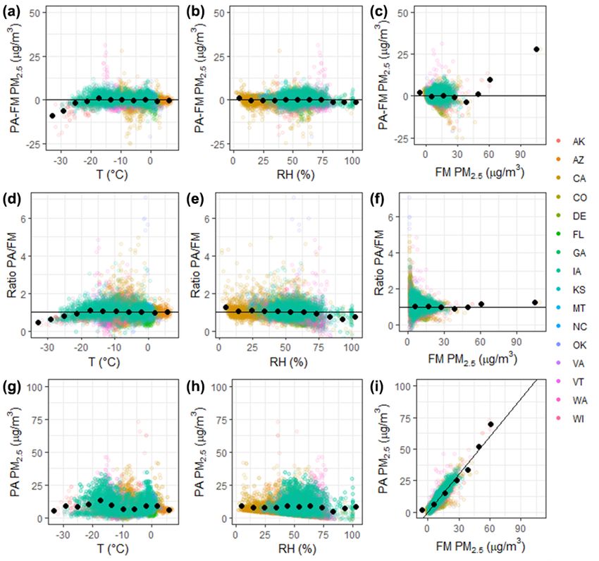
K. K. Barkjohn et al.: Development and application of a United States-wide correction for PM2.5 data                     4621

pleteness was used for the PurpleAir data as they likely have   (2 SD = 61 %) were flagged for removal. At low concentra-
more error than FEM or FRM measurements.                        tions, where a difference of a few micrograms per cubic me-
                                                                ter could result in a percent error greater than 100 %, an ab-
3.2.2   PurpleAir temperature and RH errors                     solute concentration difference threshold of 5 µg m−3 , pre-
                                                                viously proposed by Tryner et al. (2020a), was effective at
For correction model development, it was important              removing questionable observations but was not appropriate
to start with the most robust dataset possible. In the          at higher concentrations, where a 5 µg m−3 difference was
2 min or 80 s data, occasionally, an extremely high value       more common but only represents a small percent difference.
(i.e., 2 147 483 447) or an extremely low value (i.e., −224     Therefore, data were cleaned using a combination of these
or −223) was reported, likely due to electrical noise or a      metrics; data were considered valid if the difference between
communication error between the temperature sensor and          channels A and B was less than 5 µg m−3 or 61 %.
the PurpleAir microcontroller. The high error occurred in          As illustrated in Fig. 1, 24 h averaged PM2.5 concentra-
24 of 53 sensors but occurred infrequently (34 instances in     tions reported by channels A and B generally agree excep-
∼ 107 points total), while the low error impacted only two      tionally well (e.g., AZ1 sensor). However, our observations
sensors (1 % of the full dataset). Temperature values above     suggest there are some sensors where the two channels show
540 ◦ C (1000 ◦ F) were excluded before calculating daily av-   a systematic bias out of the box (AK3 is the most apparent
erages since temperature errors were extreme and easily de-     example), one channel reports zeros (e.g., CA4), or reported
tected above this level. After excluding these values, rea-     concentrations do not match for a time but then recover (e.g.,
sonable 24 h averaged temperature values were generated         KS2). For this work, 24 h averages were excluded from the
(min = −25 ◦ C, max = 44 ◦ C). Future work may wish to ap-      dataset when the PurpleAir A and B channel [cf_1] PM2.5
ply a narrower range of acceptable temperature ranges, ac-      concentrations differed by more than 5 µg m−3 and 61 %.
counting for typical ambient conditions and the potential for   This resulted in removal of 0 %–47 % of the data from indi-
increased heat build-up inside sensors (discussed further in    vidual sensors (Fig. 1, Table S6) and 2.1 % of the data in the
Sect. 4.1). Similarly, the RH sensor occasionally read 255 %;   full dataset. Most sensors had little to no removal (N = 48,
this problem was experienced by each sensor at least once       < 10 % removed); five sensors had 10 % to 47 % removed
but still occurred infrequently (1083 points out of ∼ 107 to-   (AK2, AK3, CA4, CA7, WA5). Of these sensors, three had
tal). No other values were found outside 0 %–100 % in the       average channel differences of more than 25 % (27 %–45 %)
2 min or 80 s data before averaging. These points were re-      after applying 24 h A–B channel comparison removal crite-
moved from the analysis before 24 h averaging.                  ria (AK3, CA7, WA5). These sensors, representing 3 % of
   Missing temperature or RH impacted only 2 % of the           the dataset, were removed from further analysis because of
dataset (184 points), with eight sensors having one to four     the additional error they could add into the correction model
24 h averages with missing temperature or RH. One sensor,       building. In some cases, additional quality assurance checks
WI4, had 167 d (90 %) without temperature data. Most of         on either the part of PurpleAir or the purchaser could identify
the available temperature data were recorded in the first few   problem sensors before they were deployed, but this would
weeks of operation. It is unclear what caused the temperature   not catch all issues as many occurred after sensors had op-
data to be missing. All 184 points were missing temperature,    erated for a while. In addition, when errors occur between
but only 17 were also missing RH (0.2 % of full dataset).       channels some agencies cleaned the sensors with canned air
                                                                or vacuums as recommended by PurpleAir.
3.2.3   Comparison of A and B channels
                                                                   Previous work with PurpleAir sensors excluded sensors
                                                                for poor Pearson correlations, but our work shows that a more
The two Plantower sensors within the PurpleAir sensor
                                                                targeted approach may be more efficient for ensuring good-
(channels A and B) can be used to check the consistency of
                                                                quality data. Previous work with PurpleAir sensors reported
the data reported. All comparisons in this work have occurred
                                                                that 7 of 30 sensors (23 %) were defective out of the box and
at 24 h averages. Anecdotal evidence from PurpleAir sug-
                                                                exhibited low Pearson correlations (r < 0.7) in a laboratory
gests some disagreements may be caused by spiders, insects,
                                                                evaluation (Malings et al., 2020). A total of 10 of 53 sensors
or other minor blockages that may resolve on their own. Data
                                                                (19 %) in our study had r < 0.7 at 24 h averages (i.e., AK2,
cleaning procedures were developed using the typical 24 h
                                                                CA3, CA4, CA7, IA10, KS2, WA2, WA3, WA5, WI2); only
averaged agreement between the A and B channels expressed
                                                                2 of these were removed due to large average percent differ-
as percent error (Eq. 1).
                                                                ences after removing outliers where A and B channels did
                            (A − B) × 2                         not agree (i.e., WA5, CA7); 6 of these 10 sensors had ≤ 4 %
24 h percent difference =               ,                 (1)   of the data removed by data cleaning steps, and their Pear-
                              (A + B)
                                                                son correlation, on 24 h averages, improved to ≥ 0.98 (from
where A and B are the 24 h average PM2.5 cf_1 concentra-        r < 0.7), suggesting that the low correlation was driven by
tions from the A and B channels; 24 h averaged data points      a few outlier points. Some sensors with low initial Pearson
with percent differences larger than 2 standard deviations      correlations had high Spearman correlations (range: 0.69 to

https://doi.org/10.5194/amt-14-4617-2021                                         Atmos. Meas. Tech., 14, 4617–4637, 2021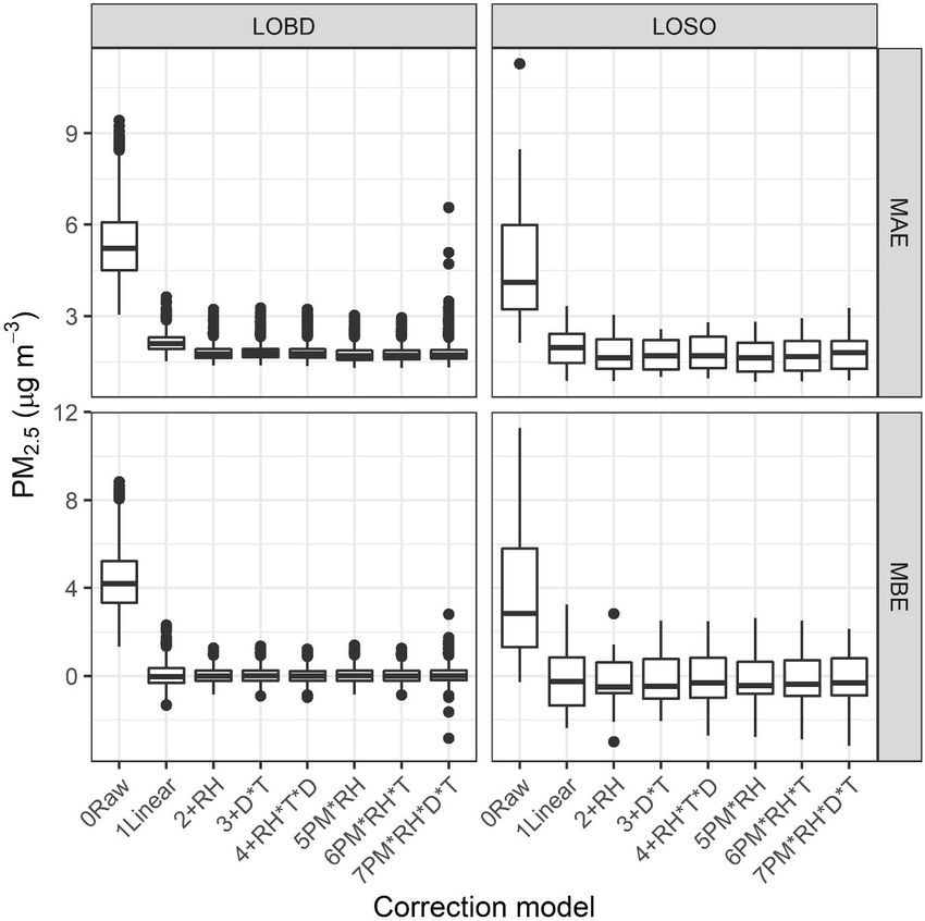
4622              K. K. Barkjohn et al.: Development and application of a United States-wide correction for PM2.5 data

                                                                  and B channel comparison on the 24 h averaged data points
                                                                  (e.g., 5 µg m−3 and 61 %) may be sufficient.

                                                                  3.3    Data summary

                                                                  After excluding poorly performing sensors (N = 3), 50 Pur-
                                                                  pleAir sensors were used in this analysis. These sensors were
                                                                  located in 16 states across 39 sites (Fig. 2, Table 1). Some
                                                                  sites had several PurpleAir sensors running simultaneously
                                                                  (N = 9), and one ran multiple sensors in series (i.e., one sen-
                                                                  sor failed and was removed, and another sensor was put up in
                                                                  its place). Some states had more than 2 years of data, while
                                                                  others had data from a single week or season. Median state-
                                                                  by-state PM2.5 concentrations, as measured by the FRM or
                                                                  FEM, ranged from 4–10 µg m−3 . A wide range of PM2.5 con-
                                                                  centrations was seen across the dataset, with a maximum 24 h
                                                                  average of 109 µg m−3 measured in California; overall the
                                                                  median PM2.5 concentration of the dataset was 7 µg m−3 (in-
                                                                  terquartile range: 5–11 µg m−3 , average (SD): 9 (5) µg m−3 ).
                                                                  These summary statistics were calculated after selecting a
                                                                  random subset of the Iowa data. The median of the Iowa
                                                                  dataset increased from 7 to 10 µg m−3 after subsetting since
Figure 1. Comparison of 24 h averaged PM2.5 data from the Pur-
pleAir A and B channels. Excluded data (2.1 %) are shown in red
                                                                  more of the high-concentration data were conserved. Sensors
and represent data points where channels differed by more than    were located in several US climate zones (NOAA, 2020; Karl
5 µg m−3 and 61 %. AK3, CA7, and WA5 were excluded from fur-      and Koss, 1984), resulting in variable temperature and RH
ther analysis. Pearson correlation (r) is shown on each plot.     ranges (Fig. S5). There were limited data above 80 % RH as
                                                                  measured by the PurpleAir RH sensor, which, as discussed
                                                                  in the following section, is known to consistently report RH
                                                                  lower than ambient.
0.98); this suggests, again, that the low performance was due
to a few outlier points. These results highlight that sensors
may fail checks based on Pearson correlation or overall per-      4     Model development
cent difference thresholds due to only a small fraction of
points, often making them poor indicators of overall sensor       4.1    Model input considerations
performance. The removal of outliers after comparing the A
                                                                  To build a data correction model that could easily be applied
and B channels can greatly improve agreement between sen-
                                                                  to all PurpleAir sensors, only data reported by the PurpleAir
sors and between sensors and reference instruments.
                                                                  sensor (or calculated from these parameters) were considered
                                                                  as model inputs. The 24 h FRM or FEM PM2.5 concentra-
3.2.4   Importance of PurpleAir data cleaning                     tions were treated as the independent variable (plotted on
        procedures                                                the x axis), allowing the majority of error to reside in the
                                                                  PurpleAir concentrations. We considered a number of redun-
This work did not seek to optimize data cleaning procedures       dant parameters (i.e., multiple PM2.5 measurements, multiple
to balance data retention with data quality; instead it fo-       environmental measurements), and we considered a number
cused on generating a best-case dataset from which to build       of increasingly complex models where parameters that were
a model. However, the removal of outlier points based on the      not strongly correlated were included as additive terms with
difference between the A and B channels appears to reduce         coefficients or where they were multiplied with each other
the errors most strongly (Supplement Sect. S3, Table S7)          to form more complex models, accounting for collinearity.
when compared to removing incomplete daily averages or re-        Increasingly complex models were evaluated based on the
moving problematic sensors. Since both channels are needed        reduction in root mean square error (RMSE; Eq. S1). Sub-
for comparison, it makes sense to average the A and B chan-       sequently, several of the best-performing model forms were
nels to improve the certainty in the measurement. The data        validated using withholding methods as described in the next
completeness control provides less benefit and may not be         section.
needed for all future applications of these correction meth-         In a multiple linear regression, all independent variables
ods. In addition, sensors with systematic offsets were uncom-     should be independent; however, much previous work has
mon and did not largely impact the overall accuracy, so the A     used models that incorporate additive temperature, RH, and

Atmos. Meas. Tech., 14, 4617–4637, 2021                                            https://doi.org/10.5194/amt-14-4617-2021
K. K. Barkjohn et al.: Development and application of a United States-wide correction for PM2.5 data 4623
Figure 2. State, local, and tribal (SLT) air monitoring sites with collocated PurpleAir sensors, including regions used for correction model
evaluation.
Table 1. Summary of the dataset used to generate the US-wide PurpleAir correction equation after three sensors with large A–B channel
discrepancies were removed. PM2.5 concentrations from both the FEM or FRM and the raw PurpleAir (PA), temperature (T ) and relative
humidity (RH), are summarized as median (min, max).
State Start date End date No. of No. of No. of FEM or FEM or FRM PA PA PA
(mm/dd/yyyy) (mm/dd/yyyy) PA Sites points FRM PM2.5 PM2.5 T (◦ C) RH (%)
(µg m−3 ) (µg m−3 )
CA 11/29/2017 12/29/2019 13 12 3762 Both 6 (−2, 109) 7 (0, 250) 22 (6, 42) 45 (2, 100)
IA 9/29/2017 1/13/2020 9 5 3762 Both 10 (0, 36) 19 (0, 69) 11 (−27, 35) 55 (21, 100)
WA 10/16/2017 10/28/2019 3 3 1035 FEM 6 (0, 41) 8 (0, 89) 13 (−2, 30) 63 (26, 84)
AZ 11/9/2018 12/31/2019 3 3 895 Both 7 (1, 43) 6 (0, 74) 24 (9, 44) 26 (5, 73)
WI 1/1/2019 11/18/2019 6 4 811 Both 6 (1, 32) 9 (1, 64) 18 (−25, 33) 53 (31, 82)
NC 3/25/2018 10/24/2019 1 1 700 Both 7 (0, 20) 13 (1, 43) 25 (−1, 35) 48 (16, 79)
AK 11/7/2018 9/30/2019 3 1 369 FRM 4 (0, 60) 4 (0, 131) 8 (−25, 29) 47 (21, 76)
KS 3/13/2019 9/30/2019 3 1 306 FEM 9 (2, 33) 11 (0, 50) 24 (9, 34) 52 (30, 71)
DE 7/27/2019 11/18/2019 1 1 205 Both 7 (1, 17) 9 (1, 35) 25 (6, 35) 51 (34, 75)
OK 7/10/2019 11/18/2019 2 2 190 Both 9 (1, 25) 11 (1, 35) 30 (1, 38) 57 (29, 86)
GA 8/2/2019 11/18/2019 1 1 184 Both 9 (3, 18) 15 (5, 34) 29 (5, 36) 55 (44, 77)
VT 3/30/2019 9/30/2019 1 1 146 Both 6 (2, 18) 8 (1, 31) 24 (12, 34) 52 (36, 71)
FL 5/31/2019 9/30/2019 1 1 119 FEM 6 (3, 17) 5 (1, 25) 32 (29, 35) 60 (49, 73)
CO 8/22/2019 11/18/2019 1 1 113 Both 7 (2, .25) 6 (1, 45) 18 (−5, 32) 33 (18, 70)
VA 10/27/2019 12/29/2019 1 1 30 FRM 5 (2, 20) 10 (2, 41) 12 (8, 25) 48 (35, 65)
MT 12/3/2019 12/10/2019 1 1 8 FEM 10 (5, 15) 22 (6, 36) 4 (2, 6) 54 (42, 62)
All 9/29/2017 1/13/2020 50 39 12 635 both 7 (−2, 109) 10 (0, 250) 19 (−27, 44) 51 (2, 100)
dew point terms that are not independent (Magi et al., 2019; tion between the delta of each bin (e.g., particles > 0.3 µm
Malings et al., 2020). We have not considered these mod- – particles > 0.5 µm = particles 0.3–0.5 µm). The delta bin
els and have considered models with interaction terms (i.e. counts were still moderately to strongly correlated (r = 0.6–
RH × T ×PM2.5 ) to account for interdependence between 1), with the weakest correlation seen between the smallest
terms instead. Strong correlations (r ≥ ±0.7) are shown be- and largest bins (Fig. S7). Moderate correlations (r = ±0.4–
tween the 24 h averaged FEM or FRM PM2.5 , PurpleAir- 0.6) are seen between temperature, RH, and dew point. Weak
estimated PM2.5 (cf_1and cf_atm), and each binned count correlations (r ≤ ±0.2) are seen between the PM variables
(Fig. S6). Since the binned counts include all particles (i.e., PM2.5 and bin variables) and environmental variables
greater than a certain size, we also consider the correla- (i.e., temperature, RH, and dew point). The correlation be-
https://doi.org/10.5194/amt-14-4617-2021 Atmos. Meas. Tech., 14, 4617–4637, 20214624 K. K. Barkjohn et al.: Development and application of a United States-wide correction for PM2.5 data
tween variables was considered when considering model PurpleAir-measured meteorology. Although not as accurate
forms. as the reference measurements, the PurpleAir temperature
For PM, we considered PM2.5 concentrations from both and RH measurements are good candidates for inclusion in
the [cf_1] and [cf_atm] data columns as model terms. Pre- a linear model because they are well correlated with refer-
vious work has found different columns to be more strongly ence measurements and may more closely represent the par-
correlated under different conditions (Barkjohn et al., 2020; ticle drying that occurs inside the sensor. In addition, using
Tryner et al., 2020a). Previous studies have suggested that onboard measurements and information that would be avail-
the binned particle count data from the Plantower are more able for all PurpleAir sensors allows us to gather corrected air
effective at estimating PM2.5 concentrations than the re- quality data from all PurpleAirs, even those in remote areas
ported PM2.5 concentration data from the newer Plantower far from other air monitoring or meteorological sites.
PMSA003 sensor (Zusman et al., 2020). However, the bins
are highly correlated, and so multilinear equations with ad- 4.1.1 Selecting models
ditive terms representing the bins were not considered.
Temperature, RH, and dew point, as calculated from the RMSE was used to determine the best models of each in-
reported temperature and RH data, were also considered creasing level of complexity moving forward (Table 2). The
based on previous studies (Malings et al., 2020). Dew point PM2.5 [cf_1] data resulted in less error than the [cf_atm]
was considered since past work has shown that dew point (Fig. 3) across all model forms (Table 2). The modest change
can, in some cases, explain error unexplained by temperature in RMSE reflects the fact that only 3.8 % of the dataset has
or RH (Mukherjee et al., 2019; Malings et al., 2020). Pres- FRM or FEM PM2.5 concentrations greater than 20 µg m−3 ,
sure was not a reported variable for 10 % of the dataset and which is where these two data columns exhibit a different
was therefore not considered as a possible correction param- relationship. Previous work with Plantower sensors in the
eter. US has shown nonlinearity at higher concentrations > 10–
Both linear and nonlinear RH terms were considered. 25 µg m−3 , which we do not see, which appears due to the
Previous studies often used a nonlinear correction for RH use of the [cf_atm] data in the previous work (Stampfer et
as opposed to a correction that changes linearly with RH al., 2020; Kelly et al., 2017; Malings et al., 2020).
(Stampfer et al., 2020; Tryner et al., 2020a; Kim et al., 2019; The next most complex model considered adding a sin-
Malings et al., 2020; Zheng et al., 2018; Lal et al., 2020). A gle additive term representing the meteorological variables.
nonlinear RH model was tested by adding an RH2 / (1 − RH) Including an additive, linear RH term to a model al-
term (see Eq. 3) similar to what has been used in past work ready including the [cf_1] PurpleAir PM2.5 data yielded
for Plantower sensors and other light scattering measure- the lowest error (RMSE = 2.52), with dew point reduc-
ments (Tryner et al., 2020a; Malings et al., 2020; Chakrabarti ing error less than temperature (+ D RMSE = 2.86 µg m−3 ,
et al., 2004; Zheng et al., 2018; Zhang et al., 1994; Day and + T RMSE = 2.84 µg m−3 ). Since the linear model with RH
Malm, 2001; Soneja et al., 2014; Lal et al., 2020; Barkjohn has the best performance of these combinations, it will be
et al., 2021). In Eq. (2), PA is the PurpleAir PM2.5 data, and further considered in the next section.
PM2.5 is the concentration provided by the collocated FRM As in previous studies with Plantower sensors, the Pur-
or FEM. pleAir sensors appear to overestimate PM2.5 concentrations
at higher RH (Tryner et al., 2020a; Magi et al., 2019; Mal-
RH2 ings et al., 2020; Kim et al., 2019; Zheng et al., 2018). Over-
PA = s1 × PM2.5 + s2 × PM2.5
(1 − RH) estimation was observed in our dataset before correction as
RH2 shown in Figs. S8 and S9, with overestimation increasing be-
+ s3 × +i (2) tween 30 % and 80 %. There are few 24 h averages above
(1 − RH)
80 % RH, so there is more uncertainty in the relationship
It is important to note that the meteorological sensor in above that level, although it appears to level off. However,
the PurpleAir sensor is positioned above the particle sen- the RH2 / (1 − RH) had higher error than using the same
sors nestled under the PVC cap, resulting in temperatures equation with just RH (nonlinear RH: RMSE = 2.86 µg m−3 ;
that are higher (2.7 to 5.3 ◦ C) and RH that is drier (9.7 % + RH term: RMSE = 2.52 µg m−3 ), so this model form will
to 24.3 %) than ambient conditions (Holder et al., 2020; not be used moving forward. This result suggests that there
Malings et al., 2020). In addition, these internal measure- may be other variations in aerosol properties and meteorol-
ments have been shown to be strongly correlated with ref- ogy in this nationwide dataset which are not well captured
erence temperature and RH measurements with high preci- just by considering hygroscopicity. This term may be more
sion (Holder et al., 2020; Tryner et al., 2020a; Magi et al., significant in localized areas with high sulfate and nitrate
2019). The well-characterized biases and strong correlations concentrations, where aerosol hygroscopicity plays an im-
between PurpleAir and ambient meteorological parameters portant role.
mean that the coefficients using these terms in a correction More complex models which add terms to account for in-
equation account for the differences between the ambient and teractions between environmental conditions were also con-
Atmos. Meas. Tech., 14, 4617–4637, 2021 https://doi.org/10.5194/amt-14-4617-2021K. K. Barkjohn et al.: Development and application of a United States-wide correction for PM2.5 data 4625
Table 2. Correction equation forms considered and the root mean square error (RMSE). The best-performing model from each increasing
level of complexity (as indicated with ∗ ) was validated using withholding methods in the next sections (Sect. 5).
Name Equation RMSE (µg m−3 ) RMSE (µg m−3 )
(cf_1) (cf_atm)
Linear PA = PM2.5 × s1 + b 2.88∗ 3.01
+ RH PA = s1 × PM2.5 + s2 × RH + i 2.52∗ 2.59
+T PA = s1 × PM2.5 + s2 × T + i 2.84 2.96
+D PA = s1 × PM2.5 + s2 × D + i 2.86 2.99
+RH × T PA = s1 × PM2.5 + s2 × RH + s3 × T + s4 × RH × T + i 2.52 2.60
+RH × D PA = s1 × PM2.5 + s2 × RH + s3 × D + s4 × RH × D + i 2.52 2.60
+D × T PA = s1 × PM2.5 + s2 × D + s3 × T + s4 × D × T + i 2.51∗ 2.61
+RH × T × D PA = s1 × PM2.5 + s2 × RH + s3 × T + s4 × D + s5 × RH × T 2.48∗ 2.57
+s6 × RH × D + s7 × T × D + s8 × RH × T × D + i
PM × RH PA = s1 × PM2.5 + s2 × RH + s3 × RH × PM2.5 + i 2.48∗ 2.53
PM ×T PA = s1 × PM2.5 + s2 × T + s3 × T × PM2.5 + i 2.84 2.96
PM ×D PA = s1 × PM2.5 + s2 × D + s3 × D × PM2.5 + i 2.86 3.00
RH2 RH 2
PM × nonlinear RH PA = s1 × PM2.5 + s2 (1−RH) × PM2.5 + s3 × (1−RH) +i 2.86 2.99
PM ×RH × T PA = s1 × PM2.5 + s2 × RH + s3 × T + s4 × PM2.5 × RH 2.46∗ 2.53
+s5 × PM2.5 × T + s6 × RH × T + s7 × PM2.5 × RH × T + i
PM ×RH × D PA = s1 × PM2.5 + s2 × RH + s3 × D + s4 × PM2.5 × RH 2.54 2.57
+s5 × PM2.5 × D + s6 × RH × D + s7 × PM2.5 × RH × D + i
PM ×T × D PA = s1 × PM2.5 + s2 × T + s3 × D + s4 × PM2.5 × T 2.52 2.63
+s5 × PM2.5 × D + s6 × T × D + s7 × PM2.5 × T × D + i
PM ×RH × T × D PA = s1 × PM2.5 + s2 × RH + s3 × T + s4 × D + s5 × PM2.5 × RH 2.42∗ 2.51
+s6 × PM2.5 × T + s7 × T × RH + s8 × PM2.5 × D
+s9 × D × RH + s10 × D × T + s11 × PM2.5 × RH × T
+s12 × PM2.5 × RH × D + s13 × PM2.5 × D × T
+s14 × D × RH × T + s15 × PM2.5 × RH × T × Di
Figure 3. Comparison of the 24 h raw PurpleAir (PA) cf_1 and cf_atm PM2.5 outputs (a) and both outputs compared to the FEM or FRM
PM2.5 measurements (b, c) across all sites, with the 1 : 1 line in red.
sidered (Table 2, rows 6–9). Lower error was observed more, with PM × RH having the lowest error for a sin-
for the +D × T (RMSE = 2.51 µg m−3 ) compared to other gle interaction term (RMSE = 2.48 µg m−3 ), although the
models of similar complexity, and slightly lower error error was similar to the +RH × T × D model. Adding a
was observed when adding RH as well (+RH × T × D second interaction term for T explains slightly more error
RMSE = 2.48 µg m−3 ). Adding interaction terms between (PM ×RH× T RMSE = 2.46 µg m−3 ), and the most error is
PM2.5 and the environmental conditions reduced error even explained by the most complex model (PM ×RH× T × D
https://doi.org/10.5194/amt-14-4617-2021 Atmos. Meas. Tech., 14, 4617–4637, 20214626 K. K. Barkjohn et al.: Development and application of a United States-wide correction for PM2.5 data
RMSE = 2.42 µg m−3 ). These best-performing models are 5 Model evaluation
further considered in the next section.
5.1 Model validation methods
4.1.2 Models considered
Building the correction model based on the full dataset could
Based on this analysis, the seven models with the lowest lead to model overfitting, so two different cross-validation
RMSE were explored further. In those equations, shown be- structures were used: (1) “leave out by date” (LOBD) and
low, PA represents the PurpleAir PM2.5 [cf_1] data, PM2.5 (2) “leave one state out” (LOSO). For the LOBD model vali-
represents the PM2.5 concentration provided by the collo- dation method, the project time period was split into 4-week
cated FRM or FEM, s1 –s7 are the fitted model coefficients, i periods, with the last period running just short of 4 weeks
is the fitted model intercept, and RH and T represent the RH (24 d). Each period contained between 179 and 2571 24 h
and temperature as measured by the PurpleAir sensors. data points, with typically more sensors running continu-
1. Simple linear regression ously during later chunks as more sensors were deployed
and came online over time. Thirty periods were available
PA = s1 × PM2.5 + i (3) in total, and, for each test-train set, 27 periods were used to
train the correction model, while three periods were selected
2. Multilinear with an additive RH term to test the correction model. Models were generated for all
27 000 combinations of test data. For the LOSO model vali-
PA = s1 × PM2.5 + s2 × RH + i (4) dation method, the correction model was built based on sen-
sors from all but one state, and then the model was tested
3. Multilinear with additive T and D interaction terms on data from the withheld state. This resulted in 16 unique
models since there are 16 states represented in this dataset.
PA = s1 × PM2.5 + s2 × D + s3 × T + s4 × D × T + i (5) The LOSO method is useful for understanding how well
the proposed correction may work in geographic areas that
4. Multilinear with additive and multiplicative terms using are not represented in our dataset. The performance of each
RH, T , and D correction method on the test data was evaluated using the
RMSE, the mean bias error (MBE), the mean absolute er-
PA = s1 × PM2.5 + s2 × RH + s3 × RH × PM2.5 + i (6) ror (MAE), and the Spearman correlation (ρ). Equations for
these statistics are provided in the Supplement (Sect. S1).
5. Multilinear with additive and multiplicative terms using To compare statistical difference between errors, t tests were
RH and PM2.5 used to compare normally distributed datasets (as determined
by Shapiro–Wilk), and Wilcoxon signed rank tests were used
PA = s1 × PM2.5 + s2 × RH + s3 × RH × PM2.5 + i (7) for nonparametric datasets with a significance value of 0.05.
Both tests were used in cases where results were marginal.
6. Multilinear with additive and multiplicative terms using
T , RH, and PM2.5 5.2 Model evaluation
PA = s1 × PM2.5 + s2 × RH + s3 × T Figure 4 shows the performance of the raw and corrected Pur-
+ s4 × PM2.5 × RH + s5 × PM2.5 × T pleAir PM2.5 data using the seven proposed correction mod-
+ s6 × RH × T + s7 × PM2.5 × RH × T + i (8) els for datasets of withheld dates (LOBD) or states (LOSO).
Both MBE, which summarizes whether the total test dataset
7. Multilinear with additive and multiplicative terms using measures higher or lower than the FRM or FEM measure-
T , RH, D, and PM2.5 ments, and MAE, which summarizes the error in 24 h aver-
ages, are shown, with additional statistics and significance
PA = s1 × PM2.5 + s2 × RH + s3 × T + s4 × D testing shown in the Supplement (Tables S8, S9). Large re-
+ s5 × PM2.5 × RH + s6 × PM2.5 × T ductions in MAE and MBE are seen when applying a linear
correction (Eq. 3). Using LOBD, the MBE across withhold-
+ s7 × T × RH + s8 × PM2.5 × D ing runs drops significantly from 4.2 to 0 µg m−3 , with a sim-
+ s9 × D × RH + s10 × D × T ilar significant drop, from 2.8 to 0 µg m−3 , for LOSO with-
+ s11 × PM2.5 × RH × T holding as well. This is a large improvement considering the
+ s12 × PM2.5 × RH × D average concentration in the dataset is 9 µg m−3 . When ap-
plying an additive RH term (+ RH), the MAE improves sig-
+ s13 × PM2.5 × D × T + s14 × D × RH × T nificantly by 0.3 µg m−3 for LOBD and by 0.4 for LOSO.
+ s15 × PM2.5 × RH × T × D + i (9) Median LOSO and LOBD MBE do not change significantly.
The interquartile range (IQR) improves for both metrics and
Atmos. Meas. Tech., 14, 4617–4637, 2021 https://doi.org/10.5194/amt-14-4617-2021K. K. Barkjohn et al.: Development and application of a United States-wide correction for PM2.5 data 4627
5.3 Selected correction model
In the end, the additive RH model (Eq. 4) seems to opti-
mally summarize a wide variety of data while reducing er-
ror (MAE) compared to a simple linear correction. The fol-
lowing correction model (Eq. 10) was generated for the full
dataset, where PA is the average of the A and B channels
from the higher correction factor (cf_1), and RH is in per-
cent.
PM2.5 = 0.524 × PAcf_1 − 0.0862 × RH + 5.75 (10)
This work indicates that only an RH correction is needed
to reduce the error and bias in the nationwide dataset. Some
previous single-site studies found temperature to signifi-
cantly improve their PM2.5 prediction as well (Magi et al.,
2019; Si et al., 2020). Humidity has known impacts on the
light scattering of particles; no similar principle exists for
explaining the influence of temperature on particle light scat-
tering. Instead, the temperature factor may help account for
some local seasonal or diurnal patterns in aerosol properties
Figure 4. Performance statistics including mean bias error (MBE)
within smaller geographical areas. These more local vari-
and mean absolute error (MAE) are shown by correction method
(0–7), where each point in the boxplot is the performance for either ations may be why temperature does not substantially re-
a 12-week period excluded from correction building (“LOBD”) or duce error and bias in the nationwide dataset. More work
a single state excluded from correction building (“LOSO”). should be done to better understand this influence. These pre-
vious models also did not include a term accounting for the
collinearity between temperature and relative humidity that
withholding methods, showing that models typically have may have been present. Figure 5 shows the residual error
more consistent performance across withheld datasets. Over- in each 24 h corrected PurpleAir PM2.5 measurement com-
all, the additive RH correction model improves performance pared with the temperature, RH, and FRM or FEM PM2.5
over the linear correction. concentrations. Error has been reduced compared to the raw
Increasing the complexity of the model (Eqs. 5–9) shows dataset (Figs. S8 and S9) and is unrelated to temperature,
similar performance to the additive RH model with no fur- RH, and PM2.5 variables. Some bias at very low temperature
ther improvements in MBE or RMSE for LOSO withhold- < −12 ◦ C and potentially high concentration (> 60 µg m−3 )
ing. When using the multiplicative RH model, the MAE may remain, but more data are needed to further understand
changes significantly (t test, Wilcoxon test); however, the this relationship.
median values do not largely change (1.6 µg m−3 ). However,
because this dataset contains limited high concentration with 5.3.1 The influence of FEM and FRM type
a limited range of RH experienced at higher concentration,
there is greater uncertainty in how this model would perform We briefly considered whether the use of both FEM and FRM
when extrapolated into such conditions. Therefore, the addi- measurements influenced these results. When subsetting the
tive RH model was used moving forward. However, future data to develop models using the 24 h averaged PM2.5 data
work should look at larger datasets to understand whether from only the FEM versus only the FRM, only the coefficient
a multiplicative RH correction is more appropriate. Further, for the PA slope term changed. The coefficient was slightly
model coefficients become more variable for more complex larger for FEM measurements (0.537) and smaller for FRM
models depending on the dataset that is excluded, suggesting measurements (0.492). Although the coefficients are signifi-
that individual states or short time periods may be driving cantly different (p < 0.05), they are within 10 %, leading to
some of the coefficients in the more complex models (Ta- little difference in the interpretation of PurpleAir PM2.5 mea-
ble S10). In addition, since temperature and relative humidity surements. We briefly considered whether the FEM coeffi-
are moderately correlated, they may be providing very sim- cient was driven by the T640s and found that if we build this
ilar information to the model. Since more complex models model excluding all T640 and T640x data, it is not signifi-
do not improve median MAE, MBE, or RMSE for LOSO cantly different (0.53). Concerns about error between differ-
withholding and since more complex models will be appli- ent types of FEM measurements cannot be explored using
cable for a narrower window of conditions, the additive RH this dataset. Further, FEM instruments are not randomly dis-
correction was selected as being the most robust. tributed across the US but rather clustered at sites operated
by the same air agency. Future work and a more concerted
https://doi.org/10.5194/amt-14-4617-2021 Atmos. Meas. Tech., 14, 4617–4637, 20214628 K. K. Barkjohn et al.: Development and application of a United States-wide correction for PM2.5 data
Figure 5. Error and ratio between corrected PurpleAir (PA) and FRM or FEM measurements are shown along with corrected PurpleAir
PM2.5 data (corrected using Eq. 10) as influenced by temperature, RH, and FRM or FEM PM2.5 concentration. Colors indicate states, and
black points indicate averages in 10 bins.
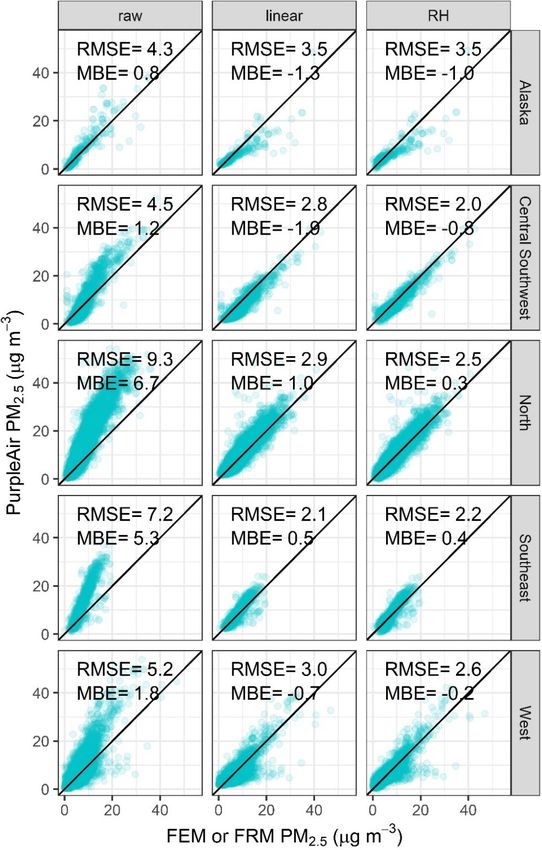
effort may be needed to explore this issue. Overall, all these formance as displayed at http://purpleair.com (last access:
FEM and FRM methods have been determined to be accu- 15 June 2021) (“raw”), with a linear correction and with the
rate enough for regulatory purposes, and so we have used all final selected additive RH correction (Eq. 10). Linear regres-
to determine our US-wide correction. Although FRM mea- sion improves the RMSE in each region, and the MBE also
surements are the gold standard, using only FRM measure- decreases in all regions except for Alaska. When adding the
ments would have severely limited our dataset. In addition, RH term to the linear regression, the bias is further reduced
the use of FEM measurements will be important in future across all regions, and the RMSE improves across all regions
work to explore the performance of this model correction at except for the southeast, where it increases slightly (< 10 %).
higher time resolutions. At higher time resolutions, the noise Alaska shows the strongest underestimate, only 1 µg m−3 on
and precision between different FEMs may impact perceived average, which appears to be driven by strong underestimates
performance, and future work should further explore this. of PM2.5 (by > 5 µg m−3 ) which occur in the winter between
November and February with subfreezing temperatures (−1
5.3.2 Error in corrected data by region to −25 ◦ C). Plantower reports that the operating range of the
sensors is −10 to 60 ◦ C, so this may contribute to the er-
The performance of the selected model is summarized by re- ror (Plantower, 2016). However, other states see subfreezing
gion. Sites were first divided by the National Oceanic and temperatures (6 % of US dataset), but most of these subfreez-
Atmospheric Administration’s (NOAA) US Climate Regions ing data from other states do not have a strong negative bias
(NOAA, 2020; Karl and Koss, 1984) and then were grouped (> 98 %), even the points that are in a similar temperature
into broader regions (Fig. 2) if the relationships between range as the Alaska data. This could suggest unique winter
the sensor and FEM or FRM measurements were not sig- particle properties or sensor performance in Fairbanks. How-
nificantly different. Uncorrected PurpleAir sensors in this ever, information on particle size distribution or composition
work overestimate PM2.5 across US regions (MBE greater is not available.
than 0 µg m−3 ; Fig. 6). Figure 6 shows the regional per-
Atmos. Meas. Tech., 14, 4617–4637, 2021 https://doi.org/10.5194/amt-14-4617-2021You can also read