CO2-equivalence metrics for surface albedo change based on the radiative forcing concept: a critical review - Recent
←
→
Page content transcription
If your browser does not render page correctly, please read the page content below
Atmos. Chem. Phys., 21, 9887–9907, 2021
https://doi.org/10.5194/acp-21-9887-2021
© Author(s) 2021. This work is distributed under
the Creative Commons Attribution 4.0 License.

CO2-equivalence metrics for surface albedo change based on the
radiative forcing concept: a critical review
Ryan M. Bright1 and Marianne T. Lund2
1 Department     of Forest and Climate, Norwegian Institute of Bioeconomy Research (NIBIO), P.O. Box 115, 1431-Ås, Norway
2 Centre   for International Climate Research (CICERO), 0349 Oslo, Norway

Correspondence: Ryan M. Bright (ryan.bright@nibio.no)

Received: 23 October 2020 – Discussion started: 10 December 2020
Revised: 3 June 2021 – Accepted: 4 June 2021 – Published: 1 July 2021

Abstract. Management of Earth’s surface albedo is increas-         1   Introduction
ingly viewed as an important climate change mitigation strat-
egy both on (Seneviratne et al., 2018) and off (Field et al.,
2018; Kravitz et al., 2018) the land. Assessing the impact         The albedo at Earth’s surface helps to govern the amount of
of a surface albedo change involves employing a measure            solar energy absorbed by the Earth system and is thus a rel-
like radiative forcing (RF) which can be challenging to di-        evant physical property shaping weather and climate (Cess,
gest for decision-makers who deal in the currency of CO2 -         1978; Hansen et al., 1984; Pielke Sr. et al., 1998). On aver-
equivalent emissions. As a result, many researchers express        age, Earth reflects about 30 % of the energy it receives from
albedo change (1α) RFs in terms of their CO2 -equivalent ef-       the sun, of which about 13 % may be attributed to the sur-
fects, despite the lack of a standard method for doing so, such    face albedo (Stephens et al., 2015; Donohoe and Battisti,
as there is for emissions of well-mixed greenhouse gases           2011). In recent years it has become the subject of increas-
(WMGHGs; e.g., IPCC AR5, Myhre et al., 2013). A major              ing research interest amongst the scientific community, as
challenge for converting 1α RFs into their CO2 -equivalent         measures to increase Earth’s surface albedo are increasingly
effects in a manner consistent with current IPCC emission          viewed as an integral component of climate change mitiga-
metric approaches stems from the lack of a universal time          tion and adaptation, both on (Seneviratne et al., 2018) and
dependency following the perturbation (perturbation “life-         off (Field et al., 2018; Kravitz et al., 2018) the land. Sur-
time”). Here, we review existing methodologies based on the        face albedo modifications associated with large-scale car-
RF concept with the goal of highlighting the context(s) in         bon dioxide removal (CDR) like re-/afforestation can detract
which the resulting CO2 -equivalent metrics may or may not         from the effectiveness of such mitigation strategies (Boysen
have merit. To our knowledge this is the first review dedi-        et al., 2016), given that such modifications generally serve to
cated entirely to the topic since the first CO2 -eq. metric for    increase Earth’s solar radiation budget, resulting in warming.
1α surfaced 20 years ago. We find that, although there are         Like emissions of GHGs and aerosols, perturbations to the
some methods that sufficiently address the time-dependency         planetary albedo via perturbations to the surface albedo rep-
issue, none address or sufficiently account for the spatial dis-   resent true external forcings of the climate system and can be
parity between the climate response to CO2 emissions and           measured in terms of changes to Earth’s radiative balance –
1α – a major critique of 1α metrics based on the RF concept        or radiative forcings (Houghton et al., 1995). The radiative
(Jones et al., 2013). We conclude that considerable research       forcing (RF) concept provides a first-order means to com-
efforts are needed to build consensus surrounding the RF “ef-      pare surface albedo changes (henceforth 1α) to other pertur-
ficacy” of various surface forcing types associated with 1α        bation types, thus enabling a more comprehensive evaluation
(e.g., crop change, forest harvest), and the degree to which       of human activities altering Earth’s surface (Houghton et al.,
these are sensitive to the spatial pattern, extent, and magni-     1995; Pielke Sr. et al., 2002).
tude of the underlying surface forcings.                              Radiative forcing is a standard measure of the effects of
                                                                   various emissions or perturbations on climate and can be

Published by Copernicus Publications on behalf of the European Geosciences Union.
9888                                     R. M. Bright and M. T. Lund: CO2 -equivalence metrics for surface albedo change

used to compare the effect of changes between any two points        a relatively new usage of the GWP metric previously unap-
in time. It is a backward-looking measure accounting for the        plied as a 1α metric – termed GWP∗ – while in Sect. 7 we
impact up to the given point and does not express the actual        review the interpretation challenges of a CO2 -eq. measure
temperature response to the perturbation. To enable aggre-          for 1α based on the RF concept. We conclude in Sect. 8
gation of emissions of different gases to a common scale,           with a discussion about the limitations and uncertainties of
the concept of CO2 -equivalent emissions is commonly used           the reviewed metrics, while providing recommendations and
in assessments, decision making, and policy frameworks.             guidance for future application.
While initially introduced to illustrate the difficulties related
to comparing the climate impacts of different gases, the field
of emission metrics – i.e., the methods to convert non-CO2          2     Radiative forcings from CO2 emissions and surface
radiative constituents into their CO2 -equivalent effects – has           albedo change
evolved and presently includes a suite of alternative formula-
                                                                    IPCC emission metrics are based on the stratospherically ad-
tions, including the global warming potential (GWP) adopted
                                                                    justed RF at the tropopause in which the stratosphere is al-
by the UNFCCC (O’Neill, 2000; Fuglestvedt et al., 2003; Fu-
                                                                    lowed to relax to the thermal steady state (Myhre et al., 2013;
glestvedt et al., 2010). Today, CO2 -equivalency metrics form
                                                                    IPCC, 2001). Estimates of the stratospheric RF for CO2
an integral part of UNFCC emission reporting and climate
                                                                    (henceforth RFCO2 ) are derived from atmospheric concen-
agreements (e.g. the Kyoto Protocol) – in addition to the
                                                                    tration changes imposed in global radiative transfer models
fields of life cycle assessment (Heijungs and Guineév, 2012)
                                                                    (Myhre et al., 1998; Etminan et al., 2016). For shortwave RFs
and integrated assessment modeling (O’Neill et al., 2016) –
                                                                    there is no evidence to suggest that the stratospheric temper-
despite much debate around GWP as the metric of choice
                                                                    ature adjusts to a surface albedo change (at least for land use
(Denison et al., 2019). As such, many researchers seek to
                                                                    and land cover change, LULCC; Smith et al., 2020; Hansen
convert RF from 1α into a CO2 -equivalent effect, which is
                                                                    et al., 2005; Huang et al. 2020), and thus the instantaneous
particularly useful in land use forcing research when pertur-
                                                                    shortwave flux change at the top of the atmosphere (TOA) is
bations to terrestrial carbon cycling often accompany the 1α.
                                                                    typically taken as RF1α , consistent with Myhre et al. (2013).
Although seemingly straightforward at the surface, the pro-
                                                                       One of the major critiques of the instantaneous or strato-
cedure is complicated by two key fundamental differences
                                                                    spherically adjusted RF is that it may be inadequate as a pre-
between 1α and CO2 : additional CO2 becomes well-mixed
                                                                    dictor of the climate response (i.e., changes to near-surface
within the atmosphere upon emission, and the resulting at-
                                                                    air temperatures, precipitation). The climate may respond
mospheric perturbation persists over millennia and cannot be
                                                                    differently to different perturbation types despite similar RF
fully reversed by human interventions. In other words, CO2 ’s
                                                                    magnitudes – or in other words – feedbacks are not inde-
RF is both temporally and spatially extensive, with the en-
                                                                    pendent of the perturbation type (Hansen et al., 1997; Joshi
suring climate response being independent of the location of
                                                                    et al., 2003). Alternative RF definitions that include tropo-
emission, whereas the RF and ensuing climate response fol-
                                                                    spheric adjustments (Shine et al., 2003) or even land surface
lowing 1α are more localized and can be fully reversed on
                                                                    temperature adjustments (Hansen et al., 2005) have been pro-
short timescales.
                                                                    posed with the argument that such adjustments are more in-
   These challenges have led researchers to adapt a vari-
                                                                    dicative of the type and magnitude of feedbacks underlying
ety of diverging methods for converting albedo change RFs
                                                                    the climate response (Sherwood et al., 2015; Myhre et al.,
(henceforth RF1α ) into CO2 equivalence. Unlike for conven-
                                                                    2013). These alternatives – referred to as “effective radia-
tional GHGs, however, there has been little concerted effort
                                                                    tive forcings (ERF)” – may be preferred when they differ no-
by the climate metric science community to build consen-
                                                                    tably from the instantaneous or stratospherically adjusted RF,
sus or formalize a standard methodology for RF1α (as evi-
                                                                    in which case their use might be preferred in metric calcu-
denced by IPCC AR4 and AR5). Here, we review existing
                                                                    lations. Alternatively, climate “efficacies” can be applied to
CO2 -equivalent metrics for 1α and their underlying meth-
                                                                    adjust instantaneous or stratospherically adjusted RF – where
ods based on the RF concept. To our knowledge this is the
                                                                    efficacy is defined as the temperature response to some per-
first review dedicated to the topic since the first 1α metric
                                                                    turbation type relative to that of CO2 . The implications of
surfaced 20 years ago. Herein, we compare and contrast ex-
                                                                    applying efficacies for spatially heterogenous perturbations
isting metrics both quantitatively and qualitatively, with the
                                                                    like 1α are discussed further in Sect. 7.
main goal of providing added clarity surrounding the context
in which the proposed metrics have (de)merits. We start in          2.1    CO2 radiative forcings
Sect. 2 by providing an overview of the methods convention-
ally applied in the climate metric context for estimating ra-       Simplified expressions for the global mean RFCO2
diative forcings following CO2 emissions and surface albedo         (in W m−2 ) due to a perturbation to the atmospheric
change. We then present the reviewed 1α metrics in Sect. 3          CO2 concentration are based on curve fits of radiative
and systematically evaluate them quantitatively in Sect. 4 and      transfer model outputs (Myhre et al., 1998, 2013):
qualitatively in Sect. 5. In Sect. 6 we review and evaluate

Atmos. Chem. Phys., 21, 9887–9907, 2021                                              https://doi.org/10.5194/acp-21-9887-2021
R. M. Bright and M. T. Lund: CO2 -equivalence metrics for surface albedo change 9889
individual physical processes. Although considered ideal for
metric calculations in IPCC AR5, state-dependent alterna-
C0 + 1C
RFCO2 (1C) = 5.35 ln , (1) tives exist in which the carbon cycle response is affected by
C0 rising temperature or CO2 accumulation in the atmosphere
where C0 is the initial concentration and 1C is the con- (Millar et al., 2017).
centration change. Because of the logarithmic relationship For an emission (or removal) scenario, RFCO2 (t) is esti-
between RF and CO2 concentration, CO2 ’s radiative effi- mated from changes to atmospheric CO2 abundance com-
ciency – or the radiative forcing per unit change in concentra- puted as a convolution integral between emissions (or re-
tion over a given background concentration – decreases with movals) and the CO2 impulse response function:
increasing background concentrations. When 1C is 1 ppm
and C0 is the current concentration, we may then refer to the Zt
solution of Eq. (1) as CO2 ’s current global mean radiative RFCO2 (t) = kCO2 e(t 0 )yCO2 (t − t 0 )dt 0 , (4)
efficiency – or αCO2 (in W m−2 ppm−1 ). t 0 =0
Updates to the RFCO2 function (Eq. 1) were given in Etmi-
nan et al. (2016) where the constant 5.35 (or RF2×CO2 / ln[2]) where t is the time dimension, t 0 is the integration variable,
was replaced by an explicit function of CO2 , CH4 , and N2 O and e(t 0 ) is the CO2 emission (or removal) rate (in kilo-
concentrations. However, this update is only important for grams).
very large CO2 perturbations and is unnecessary to consider
for emission metrics that utilize radiative efficiencies for 2.2 Shortwave radiative forcings from surface albedo
small perturbations around present-day concentrations (Et- change
minan et al., 2016).
The time step of Eq. (3) is typically 1 year; thus it is con-
For emission metrics, it is more convenient to express
venient to utilize an annually averaged RF1α when deriv-
CO2 ’s radiative efficiency in terms of a mass-based concen-
ing a CO2 -equivalent metric. Given the asymmetry between
tration increase:
solar irradiance and the seasonal cycle of surface albedo in
αCO2 εair 106 many extra-tropical regions, a more precise estimate of the
kCO2 = , (2) annual RF1α is one based on the monthly (or even daily) 1α
εCO2 Matm
(Bernier et al., 2011).
where αCO2 is the radiative efficiency per 1 ppm concen- The local annual mean instantaneous RF1α (in W m−2 )
tration increase, εCO2 is the molecular weight of CO2 following monthly surface albedo changes (unitless) can be
(44.01 kg kmol−1 ), εair is the molecular weight of air estimated with radiative kernels derived from global climate
(28.97 kg kmol−1 ), and Matm is the mass of the atmosphere models (e.g., Soden et al., 2008; Pendergrass et al., 2018;
(5.14 × 10¹⁸ kg). The solution of Eq. (2) thus yields CO2 ’s Block and Mauritsen, 2014; Smith et al., 2018), although
global mean radiative efficiency with units of W m−2 kg−1 . it should be pointed out that kernels are model- and state-
The global mean radiative forcing over time following a dependent. Bright and O’Halloran (2019) recently presented
1 kg pulse emission of CO2 can be estimated with an impulse a simplified RF1α model allowing greater flexibility sur-
response function describing atmospheric CO2 removal in rounding the prescribed atmospheric state, given as
time by Earth’s ocean and terrestrial CO2 sinks:
1 X12
− SWsfc
p
Zt RF1α (t) = m=1 ↓,m,t Tm,t 1αm,t , (5)
12
RFCO2 (t) = kCO2 yCO2 (t)dt, (3)
where 1αm,t is a surface albedo change in month m and
t=0
year t, SWsfc↓ is the incoming solar radiation flux incident
where yCO2 is a model describing the decay of CO2 at surface level in month m and year t, and Tm,t is the all-sky
in the atmosphere over time. In AR5 yCO2 is based on monthly mean clearness index (or SWsfc toa
↓ /SW↓ ; unitless) in
the multi-model mean CO2 impulse response function de- month m and year t.
scribed in Joos et al. (2013) and Myhre et al. (2013) for a It is important to reiterate that the RF1α defined with
CO2 background concentration of 389 ppmv, t is the time either Eq. (5) or kernels based on global climate models
step, and kCO2 is the radiative efficiency per kilogram of (GCMs) strictly represents the instantaneous shortwave flux
CO2 emitted upon the same background concentration (i.e., change at TOA and is not directly comparable to other defini-
1.76 × 10⁻¹⁵ W m−2 kg−1 ), which is assumed constant and tions of RF based on net (downward) radiative flux changes
time-invariant for small perturbations and for the calcula- at TOA following atmospheric adjustments. A perturbation
tion of emission metrics (Joos et al., 2013; Myhre et al., to 1α will result in a modification to the turbulent heat
2013). The pulse response function (yCO2 ) comprises four fluxes, leading to radiative adjustments in the troposphere
carbon pools representing the combined effect of several car- (Laguë et al., 2019; Huang et al., 2020; Chen and Dirmeyer,
bon cycle mechanisms rather than directly corresponding to 2020). However, in the context of emission metrics, both
https://doi.org/10.5194/acp-21-9887-2021 Atmos. Chem. Phys., 21, 9887–9907, 20219890 R. M. Bright and M. T. Lund: CO2 -equivalence metrics for surface albedo change
RF1α and RFCO2 have merit given that they do not require For this reason, Bright et al. (2016) argued that for time-
coupled climate model runs of several years to compute. dependent 1α scenarios (i.e., when 1α evolves over inter-
annual timescales), the time dependency of CO2 removal
processes (atmospheric decay) following emissions should
3 Overview of CO2 -equivalent metrics for RF1α be taken explicitly into account when estimating the effect
characterized in terms of CO2 -equivalent emissions (or re-
Over the past 20 years, a variety of metrics and their permu-
movals), thus proposing an alternate metric termed “time-
tations have been employed to express RF1α as CO2 equiv-
dependent emissions equivalence” – or T DEE:
alence, as evidenced from the 27 studies included in this re-
view (Table 1). T DEE = A−1 −1 −1 ∗
E kCO2 YCO2 RF 1α , (7)
Chiefly differentiating the methods behind the metrics
shown in Table 1 – described henceforth – is how time is where T DEE is a column vector of CO2 -equivalent emis-
represented with respect to both the 1α and the reference sion (or removal) pulses (i.e., one-offs) with length de-
gas (i.e., CO2 ) perturbations. Among the most common ap- fined by the number of time steps (e.g., years) included
proaches is to relate RF1α to the RF following a CO2 emis- in the 1α time series (in kg CO2 -eq. m−2 yr−1 ), RF ∗1α is
sion imposed on some atmospheric CO2 concentration back- a column vector of the local annual mean instantaneous
ground, but with a fraction of the emission instantaneously RF1α (in W m−2 ) corresponding to the 1α time series (or
removed by Earth’s ocean and terrestrial CO2 sinks by an RF1α (t)), and YCO2 is a lower triangular matrix with col-
amount defined by 1 minus the so-called “airborne fraction” umn (row) elements being the atmospheric CO2 fraction de-
(AF) – or the growth in atmospheric CO2 relative to anthro- creasing (increasing) with time (i.e., yCO2 (t)). The elements
pogenic CO2 emissions (Forster et al., 2007). in vector T DEE thus give the CO2 -equivalent series of
This method – or the “emissions equivalent of shortwave emission (or removal) pulses in time yielding the instan-
forcing (EESF)” – was first introduced by Betts (2000) and taneous RF1α time profile (RF1α (t)) corresponding to the
may be expressed (in kg CO2 -eq. m−2 ) as temporally explicit 1α P scenario (1α(t)). Summing all ele-
ments in T DEE (i.e., T DEE) gives a measure of the
RF1α
EESF = , (6) accumulated CO2 -eq. emissions (removals) over time. The
kCO2 AE AF T DEE approach is conceptually similar to the CO2 -forcing-
where RF1α is the local annual mean instantaneous RF from equivalence (CO2 -fe) approach (Jenkins et al., 2018; Zick-
a monthly 1α scenario (in W m−2 ), kCO2 is the global mean feld et al., 2009) building on the notion of a “forcing equiva-
radiative efficiency of CO2 (e.g., Eq. 2; in W m−2 kg−1 ), lent” index (Wigley, 1998).
AE is Earth’s surface area (5.1 × 10¹⁴ m2 ), and AF is the air- Time-dependent metrics like the well-known global warm-
borne fraction. Because AF appears in the denominator in ing potential (GWP) (Shine et al., 1990; Rogers and
Eq. (6), the CO2 -equivalent estimate will be highly sensitive Stephens, 1988) have also been applied to characterize
to the choice of AF. Figure 1 plots AF since 1959 which, as 1α(t), which accumulates RF1α (t) over time (temporally
can be seen, can fluctuate considerably over short time peri- discretized) up to some policy or metric time horizon (TH),
ods, ranging from a high of 0.81 in 1987 to a low of 0.20 in which is then normalized to the temporally accumulated ra-
1992. diative forcing following a unit pulse CO2 emission over the
More importantly, use of AF in Eq. (6) means that time- same TH:
dependent atmospheric CO2 removal processes following Pt=TH
RF1α (t)
0
emissions are not explicitly represented. However, using the GWP1α (T H ) = Pt=TH , (8)
AF may be justifiable in some contexts – such as when 1α AE kCO2 0 yCO2 (t)
has no time dependency (on inter-annual scales). For exam- where TH is the temporal accumulation or metric time hori-
ple, the pioneering study by Betts (2000) – to which almost zon. Because it is a cumulative measure, studies making use
all CO2 -eq. literature for 1α may be traced (Table 1) – made of GWP often divide by the number of time steps (TH) to ap-
use of AF when estimating CO2 equivalence of RF1α be- proximate an annual CO2 flux (e.g., Carrer et al., 2018). The
cause the research objective was to compare an albedo con- result of Eq. (8) can be interpreted as an equivalent pulse
trast between a fully grown forest and a cropland (i.e, 1α) of CO2 (in kg CO2 -eq. m−2 ) at t = 0 giving the same time-
to the stock of CO2 in the forest – a stock that had been as- integrated RF at TH as that following a 1 kg pulse of CO2 .
sumed to accumulate over 80 years, which is the approximate
time frame over which Earth’s CO2 sinks function to remove 3.1 Metric permutations
atmospheric CO2 to a level conveniently represented by the
chosen AF. Had a transient or interannual 1α scenario been Some studies have applied various permutations of the three
modeled, however, applying the EESF method at each time metrics presented above. For instance, some have applied
step of the scenario would have severely overestimated CO2 - definitions of the airborne fraction (AF) based on CO2 ’s
equivalent emissions. pulse response function (i.e., yCO2 (t)) when estimating EESF
Atmos. Chem. Phys., 21, 9887–9907, 2021 https://doi.org/10.5194/acp-21-9887-2021R. M. Bright and M. T. Lund: CO2 -equivalence metrics for surface albedo change 9891
Table 1. Studies included in this review.
Study Metric Notes
Betts (2000) EESF AF = 0.5
Akbari et al. (2009) EESF AF = 0.55
Montenegro et al. (2009) EESF AF = 0.5
Thompson et al. (2009a) EESF AF = 0.5
Thompson et al. (2009b) EESF AF = 0.5
Muñoz et al. (2010) EESF AF based on C-cycle model and TH = 20, 100, and 500 years
Menon et al. (2010) EESF AF = 0.55
Georgscu et al. (2011) EESF AF = 0.50
Cherubini et al. (2012) GWP Based on effective RF estimated with a climate efficacy of 1.94b
Bright et al. (2012) GWP
P TH = 20; 100; 500 years.
Susca, T. (2012b) T DEE
a
P
Susca, T. (2012a) T DEE
a
Guest et al. (2013) GWP
Zhao and Jackson (2014) EESF AF = 0.5; Based on effective RF estimated with a climate efficacy of 0.52c
Caiazzo et al. (2014) EESF AF based on C-cycle model and TH = 100 years
Singh et al. (2014) GWP TH = 100 years
Bright et al. (2016) T
PDEE;
T DEE
Mykleby et al. (2017) EESF AF based on C-cycle model and TH = 80 years
Fortier et al. (2017) EESF AF based on C-cycle model and TH = 100 years
Carrer et al. (2018) EESF/TH AF based on C-cycle model and TH = 100 years
Carrer et al. (2018) GWP/TH TH = 100 years
Favero et al. (2018) EESF AF based on C-cycle model and TH = 100 years
Sieber et al. (2019) GWP TH = 100 years
Sieber et al. (2020) GWP TH = 100 years
Genesio et al. (2020) EESF AF = 0.47
Sciusco et al. (2020) EESF/TH AF based on C-cycle model and TH = 100 years
Bright et al. (2020) T
PDEE;
T DEE
Lugato et al. (2020) GWP TH = 84 years
a Referred to as “time-dependent emission”. b From idealized climate model simulations of Arctic snow albedo change (Bellouin and Boucher, 2010).
c From idealized climate model simulations of global LULCC (Davin et al., 2007).
on the grounds that the analysis required a long and forward- tree for differentiating between the reviewed 1α metrics pre-
looking time perspective (Caiazzo et al., 2014; Favero et al., sented heretofore.
2018; Mykleby et al., 2017; Muñoz et al., 2010; Sciusco A principle differentiator after the time-dependency dis-
et al., 2020). A consequence is that the magnitude of the tinction is whether CO2 equivalence corresponds to a sin-
CO2 -eq. calculation is highly sensitive to the subjective gle emission (removal) pulse or a time series of multiple
choice of the TH chosen as the basis for the AF (typically CO2 -equivalent emission (removal) pulses. For the time-
taken as the mean atmospheric fraction for the period up to
R t=TH dependent metrics (Fig. 2, right branch), further distinction
TH – or TH−1 t=0 yCO2 (t)dt). Other permutations include can be made according to whether the CO2 -equivalent ef-
the normalization of EESF or GWP(TH) by TH to arrive at a fect is an instantaneous effect (in the case of the time se-
uniform time series of CO2 -eq. pulses (Carrer et al., 2018) or ries measures) and whether IPCC compatibility is desired by
the summing of T DEE up to TH to obtain a CO2 -eq. stock the practitioner (in the case of the single pulse measures).
perturbation measure (Bright et al., 2020, 2016). By “IPCC compatibility”, we mean that the metric compu-
tation and physical interpretation align with emission met-
rics presented in previous IPCC climate assessment reports
3.2 Metric decision tree and IPCC good practice guidelines for national emission in-
ventory reporting. A second or alternate distinction can be
Their relative merits and drawbacks (further discussed in made for the time-dependent and single pulse measures ac-
Sects. 4 and 5) notwithstanding, Fig. 2 presents a decision
https://doi.org/10.5194/acp-21-9887-2021 Atmos. Chem. Phys., 21, 9887–9907, 20219892 R. M. Bright and M. T. Lund: CO2 -equivalence metrics for surface albedo change
Figure 1. The 1959–2018 airborne fraction (AF), defined here as the growth in atmospheric CO2 – or the atmospheric CO2 remaining after
removals by ocean and terrestrial sinks – relative to anthropogenic CO2 emissions (fossil fuels and LULCC). “Uncertainty” is defined as
AF ± | BI |/E, where E is total anthropogenic CO2 emissions and BI is the budget imbalance – or E minus the sum of atmospheric CO2
growth and CO2 sinks. Underlying data are from the Global Carbon Project (Friedlingstein et al., 2019).
cording to whether the CO2 -equivalent effect corresponds to diative efficiencies for various forcing agents are predefined
the present (t = 0) or the future (t = TH). by the IPCC – models having origins linked to standardized
experiments employing rigorously evaluated radiative trans-
3.3 1α vs. emission metrics fer and/or climate models, which may be contrasted to the
models applied to estimate RF1α , which can vary widely in
All metric application entails subjective user decisions, such their complexity and uncertainty (for a brief review of these,
as type of metric (i.e., instantaneous vs. accumulative; scalar see Bright and O’Halloran, 2019).
vs. time series) and time horizon for impact evaluation.
CO2 -eq. metrics for 1α require additional decisions by the
practitioner affecting both their transparency and uncertainty, 4 Quantitative metric evaluation
which are highlighted in Table 2.
First among these is the need to quantify the initial physi- The metrics presented in Sect. 3 are systematically compared
cal perturbation (i.e., 1α), which is irrelevant for IPCC emis- quantitatively henceforth by deriving them for a set of com-
sion metrics where the initial perturbation is a unit pulse mon cases, starting first with the metrics applied to yield a se-
emission. For 1α metrics, uncertainty surrounding estimates ries of CO2 -eq. pulse emissions (or removals) in time. For all
of the initial (or reference) and perturbed albedo states is in- calculations, the assumed climate “efficacy” (Hansen et al.,
troduced. Second, for the time-dependent metrics (Table 2, 2005) – or the global climate sensitivity of RF1α relative to
second row) additional uncertainty is introduced by the met- RFCO2 – is 1.
ric practitioner when defining the time dependency of the
1α perturbation, which may be contrasted to IPCC emis- 4.1 CO2 -eq. pulse time series measures
sion metrics where the temporal evolution of the perturba-
tion (i.e., atmospheric concentration change) is predefined Let us first consider a geoengineering case where 1 m2 of a
(or rather, lifetimes and decay functions of the various forc- rooftop is painted white during the first year of a 100-year
ing agents). Likewise, the RF models employed to give ra- simulation, which increases the annual mean surface albedo
Atmos. Chem. Phys., 21, 9887–9907, 2021 https://doi.org/10.5194/acp-21-9887-2021R. M. Bright and M. T. Lund: CO2 -equivalence metrics for surface albedo change 9893
Table 2. Important decisions required by the practitioner to obtain a CO2 -eq. metric for 1α (based on RF) relative to conventional CO2 -
normalized emission metrics of the IPCC (i.e., GWP).
Radiative forcing agent RF metric Initial perturbation Perturbation RF model
(emission or 1α) time dependency
GWP Unit pulse IPCC IPCC
1α, time-dependent TDEE; GWP User defined User defined User defined
1α, time-independent EESF User defined None User defined
chosen, when applied in a forward-looking analysis utiliz-
ing a time-dependent 1α scenario with a time horizon of
100 years, the EESF approach underestimates the magnitude
of the annual CO2 -eq. pulse occurring in the short term rel-
ative to T DEE (Fig. 3c) and hence also RF1α in the short
term (Fig. 3b and d). This is because the CO2 forcing rep-
resented as TH−1 kCO2 AF with the EESFP approach is weaker
than the CO2 forcing represented as kCO2 t=TH
t=0 yCO2 (t) with
the T DEE approach in the short term. For higher AF val-
ues, annual CO2 -eq. removals estimated using the EESF-
based approach will underestimate the RF1α at each time
step (Fig. 3d), despite the higher-magnitude CO2 -eq. esti-
mate (relative to T DEE) seen in the longer term (Fig. 3c).
This is owed to the lower atmospheric CO2 -equivalent abun-
dance that is accumulated over the period when the series
of annual CO2 -eq. fluxes are reduced to compensate for the
higher AF.
For TH = 100 years, the EESF-based estimate will always
be lower in magnitude in the short term and higher in mag-
nitude in the longer term relative to T DEE (Fig. 3c). The
same is also true for the annual GWP-based CO2 -eq. es-
timate, although at least the reconstructed RF1α value at
Figure 2. Decision tree for 1α metrics applied in the literature in-
cluded in this review.
t = TH will always be identical to the actual RF1α value
at t = TH (Fig. 3d). In general, EESF- and GWP-based es-
timates of annualized CO2 -eq. emissions (or removals) are
sensitive to the chosen TH and will always exceed (in mag-
(Fig. 3a) for the full simulation period, resulting in a constant nitude) estimates based on T DEE. This is demonstrated in
negative RF1α (Fig. 3b). The objective is to estimate a series Fig. 4.
of CO2 -eq. fluxes associated with the local RF1α (t). The EESF-based estimate in this example is higher (in
Figure 3c presents the results after applying the relevant magnitude) than the GWP-based estimate because the as-
metrics to the common RF1α and time-dependent 1α sce- sumed AF of 0.47 is lower than the mean atmospheric frac-
nario. To assess their fidelity or “accuracy”, the resulting tion following pulse emissions (i.e., yCO2 (t)) over the range
CO2 -eq. series of annual CO2 pulses (in this case removals) of time horizons shown (the mean atmospheric fraction at
are used with Eq. (4) to re-construct the RF1α time pro- TH = 100 when applying the Joos et al. (2013) function is
file (Fig. 3b). Unsurprisingly, annual CO2 -eq. removals esti- 0.53). In contrast to the EESF- and GWP-based approaches,
mated with the T DEE approach (Fig. 3c) reproduce RF1α the magnitude of the annual CO2 -eq. removals estimated
exactly, and thus the two red curves shown in Fig. 3b and d with T DEE is insensitive to the chosen TH.
are identical (note the difference in scale). Figure 3c illus-
trates the sensitivity of the EESF-based measure derived us- 4.2 Single CO2 -eq. pulse measures
ing an AF of 0.47 (mean of the last 7 years based on the
most recent global carbon budget; e.g., Friedlingstein et al., Turning our attention to measures yielding a single CO2 -eq.
2019; Fig. 1) relative to a broad range of AF values (note emission or removal pulse, let us now consider a forest man-
that the result obtained using AF = 1 is referred to as the agement case where managers are considering harvesting a
time-independent emissions equivalent (TIEE) presented in deciduous broadleaved forest to plant a more productive ev-
Bright et al., 2016). Irrespective of the AF value that is ergreen needleleaved tree species. It is known that when the
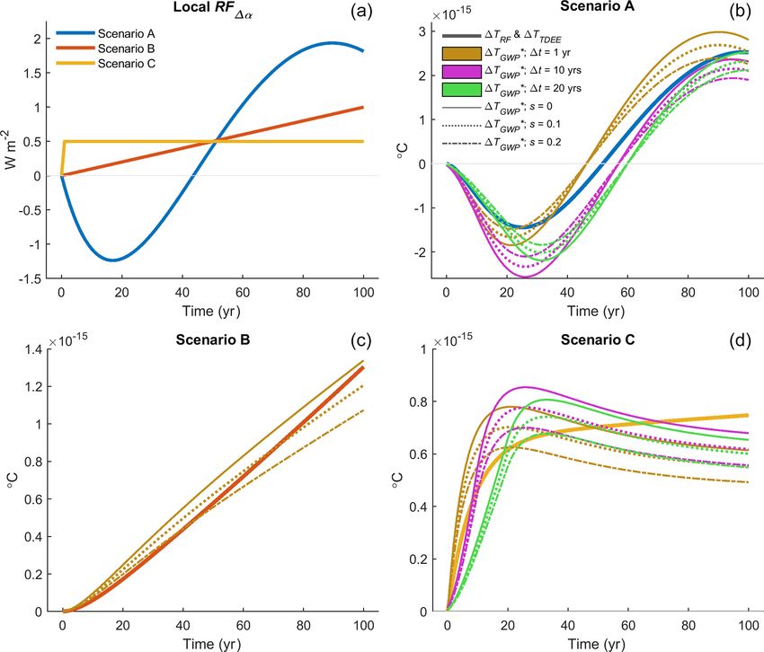
https://doi.org/10.5194/acp-21-9887-2021 Atmos. Chem. Phys., 21, 9887–9907, 20219894 R. M. Bright and M. T. Lund: CO2 -equivalence metrics for surface albedo change Figure 3. Example application of metrics yielding a complete time series of CO2 -eq. pulse emissions or removals. (a) Time-dependent local 1α scenario (“1α” = αnew −αold ). (b) The corresponding local annual mean instantaneous shortwave radiative forcing over time (RF1α (t)). (c) The derived metrics T DEE, GWP(100) / 100, and EESF / 100 for a range of airborne fractions (AF). (d) The reconstructed local annual mean RF1α (t) based on the values shown in panel (c) and Eq. (4). Note that the legend in panel (d) also applies to panel (c). evergreen needleleaved forest matures in 80 years its mean (Fig. 1). EESF estimated using AF from 2015 (Fig. 5, green annual surface albedo will be about 2 % lower than the de- diamond) is 44 % lower than EESF using AF from the pre- ciduous broadleaved forest. The corresponding annual local vious year (Fig. 5, magenta diamond). If surface albedo is RF1α at year 80 is 1.8 W m−2 , and we wish to associate a ever to be included in forestry decision making – as some CO2 equivalence with this value in order to weigh it against have proposed (Thompson et al., 2009a; Lutz and Howarth, an estimate of the total CO2 stock difference between the two 2014) – the subjective choice of the AF becomes problem- forests after 80 years (i.e., TH = 80). Assuming we have no atic given this large sensitivity. For instance, if the decision- information about how the albedo evolves a priori in the two making basis in this example depends on the net of the forests before year 80, we have no choice but to apply the CO2 -eq. of 1α and a difference in forest CO2 stock of EESF measure. 4.5 kg CO2 m−2 , adopting an AF of 0.5 might lead to a deci- Figure 5 presents the CO2 -eq. estimate based on EESF for sion to plant the new tree species given that the stock differ- an AF range of 0.1–1, shown together with an estimate in ence would exceed the EESF estimate (i.e., CO2 sinks domi- which the AF is obtained using the mean fraction of CO2 nate), whereas adopting an AF of 0.4 might lead to a decision remaining in the atmosphere at 80 years following an emis- to forego the planting given that the CO2 -eq. of 1α would sion pulse, obtained from the latest IPCC impulse response exceed the stock difference (i.e., surface albedo dominates). function (yCO2 (t)), and with the highest and lowest airborne Now let us assume the metric user does have insight into fractions of the last 7 years. how the surface albedos of both forest types will evolve over Figure 5 illustrates EESF’s sensitivity to the assumed AF. the full rotation period. In this new example, harvesting the For instance, EESF with AF = 0.3 is double that estimated deciduous broadleaf forest to plant an evergreen needleleaf with AF = 0.6 – a normal AF range for the past 60 years species will first increase the surface albedo in the short term, Atmos. Chem. Phys., 21, 9887–9907, 2021 https://doi.org/10.5194/acp-21-9887-2021
R. M. Bright and M. T. Lund: CO2 -equivalence metrics for surface albedo change                                             9895

                                                                 airborne fractions of 0.66 and lower. Similarly, the GWP-
                                                                 based estimate remembers the negative 1α occurring in the
                                                                 short term; however, GWP is a normalized measure, mean-
                                                                 ing that the time-evolving radiative effects of 1α and CO2
                                                                 are first computed independently from each other prior to
                                                                 the COP 2 -equivalence calculation, whereas for T DEE (and
                                                                 hence T DEE) CO2 equivalence depends directly on the
                                                                 time-evolving
                                                                 P               radiative effect of 1α. Framed differently,
                                                                    T DEE remembers prior CO2 -eq. fluxes yielding the ra-
                                                                 diatively equivalent effect of the time-dependent 1α sce-
                                                                 nario, whereas the “memories” of RF1α and RFCO2 underly-
                                                                 ing the GWP-based CO2 -equivalent estimate are first consid-
                                                                 ered in isolation (Fig. 6a, red curves). Hence the GWP-based
                                                                 CO
                                                                 P 2 -eq. estimate in this example is much lower than the
                                                                    T DEE-based estimate since the temporally accumulated
                                                                 RFCO2 following a unit pulse emission at t = 0 (or 6RFCO2 ,
                                                                 also known as the absolute GWP or AGW PCO2 ; Fig. 6a
Figure 4. Magnitude of the annual CO2 -eq. emission (removal)    dashed red curve) is significantly larger than the temporally
pulse as a function of the metric TH for the EESF and GWP mea-   accumulated RF1α (or 6RF1α ) representing brief periods of
sures relative to T DEE, which is insensitive to TH.             both positive and negative RF1α . Comparing brief or “short-
                                                                 lived” RFs with CO2 RFs using GWP has been heavily criti-
                                                                 cized for reasons we discuss further in Sect. 6.
                                                                    When scalar metrics are required, Fig. 6 illustrates the
                                                                 large inherent risk of applying a static measure like EESF
                                                                 to characterize 1α in dynamic systems. Moreover, for dy-
                                                                 namic systems in which 1α’s time dependency is defined
                                                                 a priori, Fig. 6 illustrates the importance of clearly defining
                                                                 the time horizon at which the physical effects of 1α and CO2
                                                                 are to be compared: GWP gives an effect measured in terms
                                                                 of
                                                                 P a present-day CO2 emission (or removal) pulse, while
                                                                    TDEE gives an effect measured in terms of a future CO2
                                                                 emission (or removal). In other words, internal consistency
                                                                 between the ecological and metric P time horizons is relaxed
                                                                 with GWP but preserved with T DEE.

                                                                 5   Qualitative metric evaluation

Figure 5. Sensitivity of EESF to the airborne fraction (AF).     The reviewed metrics and underlying methods for converting
                                                                 shortwave radiative forcings from 1α (i.e., RF1α ) into their
                                                                 CO2 -equivalent effects – summarized in Table 3 – can pri-
yet as the evergreen needleleaf forest grows and tree canopies   marily be differentiated by the physical interpretation of the
begin to close and mask the surface, the albedo difference       derived measure and by whether or not a time dependency
(1α) reverts to negative and stays negative for the remainder    (inter-annual) for 1α was defined a priori.
of the rotation. This results in an annual mean local RF1α (t)      For cases when 1α’s time dependency is not known or
profile that is first negative and then positive, which is de-   defined a priori, the EESF measure is the only applicable
picted in Fig. 6a (blue solid curve, left y axis).               measure of those reviewed, although it was shown here to be
   Converting the RF1α (t) time profile first to a time series   highly sensitive to the value chosen to represent CO2 ’s air-
of CO2 -eq. emission/removal pulses (i.e., T DEE, Fig. 6 A,      borne fraction (AF; Fig. 5) – a key input variable taking on
dashed blue curve) and then summing to year 80 gives a mea-      a wide range of values depending on how it was defined. In
sure of the totalPquantity of CO2 -eq. emitted (orPremoved)      general, when AF is defined according to historical accounts
at year 80 – or T DEE (Fig. 6b, blue curve). T DEE               of global carbon cycling, its value is prone to large fluctua-
thus “remembers” the negative 1α in the early phases of the      tions across short timescales (Fig. 1) due to natural variability
rotation period (short-term), leading to a lower CO2 -eq. es-    in the global carbon cycle (Ciais et al., 2013). When defined
timate at year 80 relative to EESF estimates computed with       as the fraction of CO2 remaining in the atmosphere following

https://doi.org/10.5194/acp-21-9887-2021                                          Atmos. Chem. Phys., 21, 9887–9907, 2021
9896 R. M. Bright and M. T. Lund: CO2 -equivalence metrics for surface albedo change
Figure 6. Example application of metrics yielding a single CO2 -eq. emission (or removal) pulse following a hypothetical forest tree species
conversion. (a) RF1α (t) and corresponding T DEE (left y axis, blue curves) and the temporally accumulated RF1α (t) normalized to
Earth’s surface area (solid red, right y axis) and temporally accumulated RFCO2 (t) (dashed red, right y axis) following a 1 kg pulse emission.
(b) EESF estimated
P for the 1α (and RF1α ) occurring at TH = 80 shown in relation to GWP(TH) – or the ratio of two red curves shown in
panel (a) – and TDEE estimated at all THs.
a pulse emission – as would be obtained from a simple car- present yielding the accumulated radiative forcing of the 1α
bon cycle model (i.e., a CO2 impulse response function) – scenario at TH years into the future. GWP has merit from
its value depends on the time horizon chosen and underly- the standpoint that it is easy to apply and conforms to estab-
ing model representation of atmospheric removal processes lished reporting methods, accounting standards, or decision-
(i.e., time constants). Use of the latter definition of AF af- support tools such as life cycle assessment (e.g., Cherubini
fixes a forward-looking time dependency to the EESF mea- et al., 2012; Sieber et al., 2020). Scientifically, however, there
sure, which is inconsistent with the definition of 1α and adds are important limitations to GWP when the forcing (i.e., 1α)
subjectivity (i.e., the choice in TH). Basing the AF on global is short-lived or temporary (Allen et al., 2016; Pierrehumbert,
carbon budget reconstructions would at least preserve some 2014; Allen et al., 2018; Lynch et al., 2020; Cain et al., 2019).
element of objectivity, although given the measure’s sensitiv- The T DEE measure, on the other hand, can be interpreted
ity to AF it would be prudent to compute the measure for a as a complete time series of CO2 emission pulses (i.e., a com-
range of AFs (i.e., as constrained by the observational record) plete emission scenario) yielding the instantaneous radiative
in an effort to boost transparency. Forgoing the use of an AF forcing of the 1α scenario. When summed to TH, the latter
altogether would eliminate all subjectivity, as has been sug- (as 6T DEE) provides a clearer indication of the radiative
gested elsewhere (Bright et al., 2016). impact incurred up to TH, thus having greater scientific merit
For cases involving a time-dependent 1α scenario that as an indicator of future warming.
is defined a priori, forward-looking measures are identified The permutations of GWP and EESF applied to arrive
whose methodological differences give rise to different in- at a time series of CO2 -eq. pulses – GWP(TH) / TH and
terpretations of CO2 equivalence (Table 3). For example, the EESF / TH – have little merit on the grounds that the result-
GWP measure can be interpreted as CO2 -eq. pulse emitted at ing series does not reproduce RF1α (t) (Fig. 3d). The T DEE
Atmos. Chem. Phys., 21, 9887–9907, 2021 https://doi.org/10.5194/acp-21-9887-2021R. M. Bright and M. T. Lund: CO2 -equivalence metrics for surface albedo change 9897
Table 3. Overview of distinguishing attributes, methodological differences, drawbacks, and merits of the six 1α metrics applied in the
scientific literature included in this review.
1α metric CO2 equivalence Time-dependent Drawbacks Merits
interpretation 1α scenario
EESF Single pulse No Sensitive to choice of airborne Easy to apply; no need to define a 1α
fraction (AF) scenario a priori
Not forward-looking
No carbon cycle dynamics
EESF/TH Series of uniform No Same as above Easy to apply
pulses CO2 -eq. series does not repro-
duce RF1α (t)a
Sensitive to TH
T DEE Series of non-uniform Yes Not scalar CO2 -eq. series reproduces RF1α (t)
pulses Can be compared to an emission sce-
nario
Insensitive to TH
6T DEE Accumulation of Yes Cannot be compared to a CO2 Compatible with policy targets based
a series of pulse of the present on cumulative emissions
non-uniform pulses Insensitive to TH
GWP Single pulse Yes Sensitive to TH Well-known; IPCC conformity
May be a poor indicator of im- Compatible with IPCC assessments
pact when 1α(t) is shorter than and UNFCCC accounting conven-
TH tions
GWP(TH)/TH Series of uniform Yes Sensitive to TH GWP method is well-known
pulses CO2 -eq. series does not repro-
duce RF1α (t) except at t = TH
a The exception is at t = TH when AF = TH−1 t=TH y
R
t=0 CO2 (t)dt .
approach was proposed to overcome this limitation, although to serve the purpose of a measure of progress towards a
it should be stressed that – like GWP(TH) / TH – its deriva- global temperature-oriented climate goal (i.e., limit warm-
tion requires that a time-dependent 1α scenario be defined ing to “well below 2 ◦ C”). Compared to conventional GWP,
a priori, which adds uncertainty and may not always be pos- cumulative CO2 -eq. emissions based on GWP∗ provide a
sible. clearer indication of future warming, and future CO2 -eq.
emission rates better indicate future warming rates. GWP∗
thus better relates all climate pollutants in a common cumu-
6 GWP∗ and 1α lative emission (or emission budget) framework, making it
easier to formulate mitigation strategies that provide a more
It is well known that the conventional usage of GWP does accurate indication of progress towards climate stabilization.
not adequately capture different behaviors of short-and long- Among one of the more distinguishing features of GWP∗
lived climate pollutants or their impact on global mean sur- is that, when applied to radiative forcings rather than pulse
face temperatures (Pierrehumbert, 2014; Allen et al., 2016; emissions, information about the time dependency of the per-
Shine et al., 2003; Fuglestvedt et al., 2010). Some have pro- turbation (i.e., the lifetimes of “climate pollutants” or forc-
posed an alternative usage of GWP – denoted GWP∗ (Allen ing agents) is not required (Lee et al., 2021; Cain et al.,
et al., 2018) – which overcomes this problem by equating an 2019; Allen et al., 2018), making it an attractive alternative
increase in the emission rate of a short-lived climate pollu- to EESF. In other words, a GWP estimate of the “short-lived”
tant (or radiative forcing agent) with a one-off “pulse” CO2 forcing agent under scope – which requires such information
emission. GWP∗ recognizes that a pulse emission of CO2 to be known or defined a priori – is unnecessary in its cal-
and a sudden step change in the sustained rate of emission culation. Only the rate of change of the forcing is required,
of a short-lived climate pollutant (SLCP) both give near- scaled by TH / AGWP(TH)CO2 as follows (Lee et al., 2021;
constant radiative forcing. Or, alternately, that a progressive Allen et al., 2018):
linear increase (or decrease) in the rate of an SLCP emis- TH
1RF1α
sion is approximately equivalent to a sustained step change ECO2 -eq.∗ = , (9)
in the emission rate of CO2 . As such, GWP∗ is considered AGWP(TH)CO2 1t
to have greater “environmental integrity” than the conven- where TH is the time horizon, AGWP(TH)CO2 is CO2 ’s
tional GWP metric (Allen et al., 2018), as it is better fit AGWP at the same TH (i.e., 9.2 × 10⁻¹⁴ W yr m−2 kg−1
https://doi.org/10.5194/acp-21-9887-2021 Atmos. Chem. Phys., 21, 9887–9907, 20219898 R. M. Bright and M. T. Lund: CO2 -equivalence metrics for surface albedo change
when TH = 100 years), 1t is the time step change, and analogous to urban expansion into a cropland (Fig. 7a, yel-
1RF1α is the time differential of RF1α (t) over the step low).
change. ECO2 -eq.∗ thus represents the CO2 -eq. emission pulse We then reconstruct the global mean temperature response
for the step change and will equal EESF when the AF (in (1T ) of the CO2 -eq.∗ emission (removal) scenario under
Eq. 6 denominator) corresponds to the mean of yCO2 (t) over varying assumptions surrounding the size of 1t and the
R t=TH
the TH (i.e., T H −1 t=0 yCO2 (t)dt). A TH of 100 years is weighting factor s (shown in Fig. 7b legend), which is then
typically applied in Eq. (9), which is justified when it ex- compared to the RF1α -based 1T and the 1T reconstructed
ceeds the lifetime of the SLCP or when the time-integrated using the CO2 -eq. emission (removal) scenario based on the
radiative forcing of the forcing agent (i.e, 1α) becomes a T DEE approach (Fig. 7b–d). For Scenario A (Fig. 7b), we
constant at this timescale, since the time-integrated radiative find no obvious parameter set that outperforms any other in
forcing of the reference gas (i.e., AGWPCO2 ) increases lin- terms of the faithfulness by which the CO2 -eq.∗ emission
early with TH. In other words, the TH dependence cancels (removal) scenario reproduces 1T across the full time hori-
out in the calculation of CO2 -eq.∗ , rendering GWP∗ insen- zon. There appears to be a trade-off between the near- and
sitive to the choice in TH, which contrasts with the conven- long-term reproduction accuracy of different parameter sets:
tional GWP (Allen et al., 2016, 2018). The step change 1t a 20-year 1t with no weighting (Fig. 7b, solid green curve)
for which 1RF is calculated is typically taken as 20 years to better reproduces the 1T response seen in the short term
“reduce the volatility of CO2 -eq.∗ emissions in response to (. 20 years) as well as the 1T seen at the end of the sce-
variations in SLCP emission rates” (Allen et al. 2018; Cain nario time horizon (year 100), whereas a 10-year 1t with no
et al. 2019), although comprehensive investigations into the weighting (Fig. 7b, solid purple curve) better reproduces the
appropriateness of this choice when applied to a wide variety 1T response seen in the longer term (from ∼ 60–90 years).
of time-varying SLCP emission (radiative forcing) scenar- An increase in the weighting factor s serves to dampen the
ios are lacking. We note that more recent works (Cain et al., amplitude between the maximum cooling and warming seen
2019; Lee et al., 2021) employed weighting-based modifica- in the short and longer term, respectively (Fig. 7b, spread be-
tions to Eq. (9) in an effort to better account for the longer- tween like-colored curves). As for Scenario B representing a
term temperature equilibration to past forcing changes: linear increase in RF, the reconstructed 1T is insensitive to
1t and thus only results for a 1-year 1t are computed and
presented in Fig. 7c. Although a weighting factor of 0.2 is
TH 1RF1α
ECO2 -eq.∗ = (1 − s) most accurate for the first ∼ 50 years, a weight of 0.1 gives
AGWP(TH) CO2 1t
a more faithful 1T reproduction for the full time period. As
RF1α for Scenario C representing a step change in RF (Fig. 7d),
+s , (10)
AGWP(TH)CO2 again we find no obvious parameter set that yields a faithful
1T reproduction across the full time period. High s weights
where s is a factor weighting the delayed response by global overpredict 1T in the medium term but reproduce 1T best
mean temperature to the radiative forcing history, repre- in the longer term (Fig. 7d, solid curves), while a 1t larger
sented here (following Lee et al., 2021) as the mean forcing than 10 years appears to result in large underpredictions in
over the period 1t – or RF1α . Note that s is analogous to the the short term (i.e., . 20 years; Fig. 7d, green curves).
“α” term seen in Eq. (1) of Lee et al. (2021) and that the fac- Unsurprisingly, 1T reconstructed using the CO2 -eq.
tor 1 − s is analogous to the rate contribution weight denoted emission (removal) scenario estimated with the T DEE ap-
as “r” in Eq. (S1) of Cain et al. (2019). Like the choice of 1t, proach exactly reproduces the RF-based 1T , and thus these
however, few investigations have been carried out to assess two estimates are plotted jointly as a single curve in Fig. 7b–
the appropriateness of weight sizes applied in Eq. (10) for d (wider solid curves). Thus, when future surface albedo
different SLCP emission (radiative forcing) scenarios having changes are defined a priori (i.e., when the 1α perturbation
widely varying temporal dynamics. “lifetime” is known or estimated), a CO2 -eq. emission (re-
We explore the sensitivity of the choice in both 1t and moval) time series quantified with T DEE is far superior
s on CO2 -eq. emissions (removals) estimated with the mod- to one based on GWP∗ irrespective of the choice in 1t or
ified GWP∗ approach (Eq. 10) for three hypothetical local weight sizes applied, making it the better CO2 -eq. measure
RF1α (t) scenarios presented in Fig. 7. The first scenario – or of progress towards global temperature stabilization.
Scenario A – is identical to the forest management scenario
plotted in Fig. 6 and extended by 20 years, which is charac-
terized by a negative RF in the short term and positive RF 7 Spatial disparity in climate response between CO2
in the longer term (Fig. 7a, blue). In the second scenario, or emissions and 1α perturbations
Scenario B, RF1α (t) corresponds to a linearly increasing 1α
trend which is loosely analogous to incremental deforestation The climate (i.e., temperature) response to a 1α perturba-
occurring on a regional scale (Fig. 7a, red). The third sce- tion either isolated (e.g., Jacobson and Ten Hoeve, 2012) or
nario, or Scenario C, resembles a permanent albedo decrease, as part of LULCC (e.g., Pongratz et al., 2010; Betts, 2001)
Atmos. Chem. Phys., 21, 9887–9907, 2021 https://doi.org/10.5194/acp-21-9887-2021R. M. Bright and M. T. Lund: CO2 -equivalence metrics for surface albedo change 9899
Figure 7. Performance of GWP∗ computed for three stylized scenarios of surface-albedo-change-driven radiative forcing using Eq. (10) with
nine different parameter sets. (a) Local radiative forcing of one permanent and two temporally evolving surface albedo change scenarios. (b–
d) The corresponding global mean temperature response 1T to the radiative forcing relative to that which has been reconstructed using the
CO2 -eq. emission (removal) time series computed with T DEE and GWP∗ under the assumption that 1αt+n−t is known. 1T in panels (b–
d) is estimated with a temperature impulse response function following Boucher and Reddy (2008) and Myhre et al. (2013) having a climate
sensitivity of 1.06 K (W m−2 )−1 , which is equivalent to a 3.9 K equilibrium climate response to an abrupt CO2 concentration doubling.
Table 4. Differences in surface property and flux perturbations between geoengineering-type forcings involving non-vegetative solar radiation
management (SRM) and forcings from LULCC, land management change (LMC), or forest management change (FMC). 1ra : change to bulk
aerodynamic resistance; 1rs : change to bulk surface resistance; 1λ(E): latent heat flux change from a change to evaporation; 1λ(E + T ):
latent heat flux change from a change to both evaporation and transpiration; 1H : sensible heat flux change.
Forcing type Surface property perturbation Surface flux perturbation
Geoengineering (non-veg. SRM) 1α 1λ(E), 1H
LULCC; LMC; FMC 1α, 1ra , 1rs 1λ(E + T ), 1H
is highly heterogeneous in space, the magnitude and ex- Nazarenko, 2004; Hansen et al., 2005; Myhre et al., 2013).
tent of which depends on its location (Brovkin et al., 2013; This has caused some researchers to question the utility of
de Noblet-Ducoudré et al., 2012). This is because the re- a CO2 -eq. measure for 1α (Jones et al., 2013) or encour-
sponse pattern of climate feedbacks has a strong spatial de- aged others to look for solutions or further methodological
pendency – feedbacks are generally larger at higher latitudes refinements. For instance, some researchers (e.g., Cherubini
due to higher energy budget sensitivity to clouds, water va- et al., 2012; Zhao and Jackson, 2014) have applied climate
por, and surface albedo, which generally increases the effec- efficacies – or the climate sensitivity of a forcing agent rela-
tiveness of RF in those regions (Shindell et al., 2015). This is tive to CO2 (Joshi et al., 2003; Hansen et al., 2005) – to adjust
in contrast to CO2 emissions where both RF and the temper- RF1α prior to the CO2 -eq. calculation. Such adjustments rec-
ature response are more homogeneous in space (Hansen and ognize that the temperature response to RF depends on the
https://doi.org/10.5194/acp-21-9887-2021 Atmos. Chem. Phys., 21, 9887–9907, 20219900 R. M. Bright and M. T. Lund: CO2 -equivalence metrics for surface albedo change geographic location, extent, and type of underlying forcing 2019; Hansen et al., 2005). Regarding the latter, most base associated with the 1α (e.g., land use and land cover change the temperature response for CO2 on the equilibrium cli- (LULCC), white-roofing), which can be co-associated with mate sensitivity (ECS) for a CO2 doubling, although good other perturbations (Table 4) like those arising from changes arguments have been made for using the transient climate to vegetative physical properties (for the LULCC case) which response (TCR) instead, particularly for short-lived forcing can modify the partitioning of turbulent heat fluxes above and agents (Marvel et al., 2016; Shindell, 2014). The tempera- beyond the purely radiatively driven change (Davin et al., ture response for the forcing agent of interest is rarely taken 2007; Bright et al., 2017). as the equilibrium response although there are some excep- Using a climate efficacy to adjust RF1α , however, is not tions (e.g. “Eα ” in Richardson et al., 2019, which is based on without its drawbacks. A first and obvious drawback is that climate feedback parameters obtained from ordinary least- efficacies are climate model dependent (Hansen et al., 2005; square regressions). Efficacies are also sensitive to the defi- Smith et al., 2020; Richardson et al., 2019). Climate models nition of RF (Richardson et al., 2019; Hansen et al., 2005). vary in their underlying physics, which is evidenced by the For example, the efficacy of sulfate forcing (5 × SO4 ) has re- large spread in CO2 ’s climate sensitivity across CMIP6 mod- cently been shown to vary from 0.94 to 2.97 depending on els (Meehl et al., 2020; Zelinka et al., 2020). A second draw- whether RF is based on the net radiative flux change at TOA back is that climate sensitivities for certain forcing agents from fixed SST experiments or the instantaneous shortwave like 1α are tied to experiments that differ largely in the way flux change at the tropopause (Richardson et al., 2019). forcings have been imposed in time and space. Both draw- Ideally, CO2 -eq. metrics based on the RF concept should backs contribute to large uncertainties in the choice of effi- be based on an RF definition yielding efficacies approach- cacy for 1α. The latter drawback is especially problematic ing unity for a broad range of forcing types. Although there since the 1α perturbation is often accompanied by perturba- is currently no consensus here, strong arguments have been tions to other surface properties and fluxes (Table 4) having made for RF definitions based on the net radiative flux large spatial and temporal dependencies. The turbulent heat change at TOA resulting from fixed SST experiments with flux perturbations that accompany a net radiative flux change GCMs and ESMs (i.e., “Fs ” in Hansen et al. 2005; “ERFSST ” at the surface affect atmospheric temperature and humidity in Richardson et al. 2019), since such definitions yield effi- profiles (Bala et al., 2008; Modak et al., 2016; Schmidt et al., cacies approaching unity for a broad range of forcing types. 2012; Kravitz et al., 2013), causing the atmosphere to ad- However, for most 1α metric practitioners it is not feasible just to a new state, resulting in a net radiative flux change at to quantify atmospheric adjustments and hence the ERF. Ef- TOA that extends beyond the instantaneous shortwave radia- ficacies compatible with RF1α (instantaneous 1SW at TOA) tive flux change (i.e., RF1α ). could be the more feasible option for metric calculations, but For example, the efficacy of LULCC forcing across the broad consensus surrounding appropriate efficacy values for six studies reviewed by Bright et al. (2015) ranged from different forcing types associated with the 1α perturbation 0.5 to 1.02 owing to differences in model set-up (e.g., fixed would need to be established first (Table 4). This is espe- SST vs. slab vs. dynamic ocean), differences in the spa- cially true for forcings involving changes to the biophysical tial extent and magnitude of the imposed LULCC forcing properties of vegetation – such as LULCC, forestry, etc. – (e.g., historical transient vs. idealized time slice), and the since these are constructs representing a seemingly myriad LULCC definition (i.e., the type of LULCC that was included combination of perturbations acting on non-radiative con- in the study such as only afforestation/deforestation vs. all trols (i.e., 1ra and 1rs ) of the surface energy balance. Build- LULCC). Even when controlling for differences in experi- ing consensus for efficacies applicable to geoengineering- mental design (e.g., CMIP protocols), the climate efficacy type forcings where the only physical property perturbed is of historical LULCC has been found to vary considerably in the surface albedo (e.g., white roofing, sea ice brightening) both sign and magnitude (see Fig. 8, Richardson et al. 2019), would be less challenging since the confounding perturba- which is more likely attributed to the larger spread in effec- tions to 1ra and 1rs and hence to the partitioning of the tur- tive radiative forcing (ERF) for LULCC than for CO2 . For bulent heat fluxes are removed. Nevertheless, irrespective of instance, Smith et al. (2020) report a standard deviation of whether broad scientific consensus can be reached surround- 6 % in the ERF of CO2 (4× abrupt) across 17 GCMs and ing efficacies suitable for 1α metrics, additional responsi- Earth system models (ESMs) participating in RFMIP in con- bility would always be imposed on the metric practitioner to trast to 175 % for LULCC, although it should be kept in mind ensure that the chosen efficacy aligns with the forcing type that the ERF is weak for LULCC and thus relative differences underlying the RF1α . become large. An additional drawback and source of uncertainty un- derlying efficacies is related to differences in their defini- tion. Differences in definition can stem from either differ- ent definitions of RF itself or differences in the definition of the temperature response per unit RF (Richardson et al., Atmos. Chem. Phys., 21, 9887–9907, 2021 https://doi.org/10.5194/acp-21-9887-2021
You can also read