Comprehensive evaluations of diurnal NO2 measurements during DISCOVER-AQ 2011: effects of resolution-dependent representation of NOx emissions ...
←
→
Page content transcription
If your browser does not render page correctly, please read the page content below
Atmos. Chem. Phys., 21, 11133–11160, 2021
https://doi.org/10.5194/acp-21-11133-2021
© Author(s) 2021. This work is distributed under
the Creative Commons Attribution 4.0 License.

Comprehensive evaluations of diurnal NO2 measurements during
DISCOVER-AQ 2011: effects of resolution-dependent
representation of NOx emissions
Jianfeng Li1,a , Yuhang Wang1 , Ruixiong Zhang1 , Charles Smeltzer1 , Andrew Weinheimer2 , Jay Herman3 ,
K. Folkert Boersma4,5 , Edward A. Celarier6,7,b , Russell W. Long8 , James J. Szykman8 , Ruben Delgado3 ,
Anne M. Thompson6 , Travis N. Knepp9,10 , Lok N. Lamsal6 , Scott J. Janz6 , Matthew G. Kowalewski6 , Xiong Liu11 ,
and Caroline R. Nowlan11
1 School of Earth and Atmospheric Sciences, Georgia Institute of Technology, Atlanta, GA, USA
2 National Center for Atmospheric Research, Boulder, CO, USA
3 Joint Center for Earth Systems Technology, University of Maryland Baltimore County, Baltimore, MD, USA
4 Royal Netherlands Meteorological Institute, De Bilt, the Netherlands
5 Meteorology and Air Quality Group, Wageningen University, Wageningen, the Netherlands
6 NASA Goddard Space Flight Center, Greenbelt, MD, USA
7 Universities Space Research Association, Columbia, MD, USA
8 National Exposure Research Laboratory, Office of Research and Development, US Environmental Protection Agency,

Research Triangle Park, NC, USA
9 NASA Langley Research Center, Virginia, USA
10 Science Systems and Applications, Inc., Hampton, VA, USA
11 Atomic and Molecular Physics Division, Harvard–Smithsonian Center for Astrophysics, Cambridge, MA, USA
a now at: Atmospheric Sciences and Global Change Division, Pacific Northwest National Laboratory,

Richland, WA, USA
b now at: Digital Spec, Tyson’s Corner, VA, USA

Correspondence: Yuhang Wang (yuhang.wang@eas.gatech.edu)

Received: 18 November 2020 – Discussion started: 6 January 2021
Revised: 1 June 2021 – Accepted: 17 June 2021 – Published: 23 July 2021

Abstract. Nitrogen oxides (NOx = NO + NO2 ) play a cru-         Instrument; GOME-2A: Global Ozone Monitoring Experi-
cial role in the formation of ozone and secondary inorganic     ment – 2A), ground-based Pandora, and the Airborne Com-
and organic aerosols, thus affecting human health, global ra-   pact Atmospheric Mapper (ACAM) instrument in July 2011
diation budget, and climate. The diurnal and spatial varia-     during the DISCOVER-AQ campaign over the Baltimore–
tions in NO2 are functions of emissions, advection, depo-       Washington region. The model simulations at 36 and 4 km
sition, vertical mixing, and chemistry. Their observations,     resolutions are in reasonably good agreement with the re-
therefore, provide useful constraints in our understanding of   gional mean temporospatial NO2 observations in the day-
these factors. We employ a Regional chEmical and trAns-         time. However, we find significant overestimations (underes-
port model (REAM) to analyze the observed temporal (di-         timations) of model-simulated NO2 (O3 ) surface concentra-
urnal cycles) and spatial distributions of NO2 concentrations   tions during nighttime, which can be mitigated by enhancing
and tropospheric vertical column densities (TVCDs) using        nocturnal vertical mixing in the model. Another discrepancy
aircraft in situ measurements and surface EPA Air Quality       is that Pandora-measured NO2 TVCDs show much less vari-
System (AQS) observations as well as the measurements of        ation in the late afternoon than simulated in the model. The
TVCDs by satellite instruments (OMI: the Ozone Monitoring       higher-resolution 4 km simulations tend to show larger bi-

Published by Copernicus Publications on behalf of the European Geosciences Union.
11134                                          J. Li et al.: Effects of resolution-dependent representation of NOx emissions

ases compared to the observations due largely to the larger       (2011) found that the diurnal patterns of surface NO, NO2 ,
spatial variations in NOx emissions in the model when the         and O3 concentrations at a tropical coastal station in In-
model spatial resolution is increased from 36 to 4 km. OMI,       dia from November 2007 to May 2009 were closely asso-
GOME-2A, and the high-resolution aircraft ACAM obser-             ciated with sea breeze and land breeze, which affected the
vations show a more dispersed distribution of NO2 vertical        availability of NOx through transport. They also thought that
column densities (VCDs) and lower VCDs in urban regions           monsoon-associated synoptic wind patterns could strongly
than corresponding 36 and 4 km model simulations, likely re-      influence the magnitudes of NO, NO2 , and O3 diurnal cycles.
flecting the spatial distribution bias of NOx emissions in the    The monsoon effect on surface NO, NO2 , and O3 diurnal cy-
National Emissions Inventory (NEI) 2011.                          cles was also observed in China by Tu et al. (2007) on the
                                                                  basis of continuous measurements of NO, NO2 , and O3 at an
                                                                  urban site in Nanjing from January 2000–February 2003.
                                                                     In addition to surface NO2 diurnal cycles, the daily varia-
1   Introduction                                                  tions in NO2 vertical column densities (VCDs) were also in-
                                                                  vestigated in previous studies. For example, Boersma et al.
Nitrogen oxides (NOx = NO + NO2 ) are among the most im-          (2008) compared NO2 tropospheric VCDs (TVCDs) re-
portant trace gases in the atmosphere due to their crucial role   trieved from OMI (the Ozone Monitoring Instrument) and
in the formation of ozone (O3 ) and secondary aerosols and        SCIAMACHY (SCanning Imaging Absorption SpectroMe-
their role in the chemical transformation of other atmospheric    ter for Atmospheric CHartography) in August 2006 around
species, such as carbon monoxide (CO) and volatile organic        the world. They found that the diurnal patterns of different
compounds (VOCs) (Cheng et al., 2017, 2018; Fisher et al.,        types of NOx emissions could strongly affect the NO2 TVCD
2016; Li et al., 2019; Liu et al., 2012; Ng et al., 2017; Peng    variations between OMI and SCIAMACHY and that intense
et al., 2016; Zhang and Wang, 2016). NOx is emitted by both       afternoon fire activity resulted in an increase in NO2 TVCDs
anthropogenic activities and natural sources. Anthropogenic       from 10:00 to 13:30 LT (local time) over tropical biomass
sources account for about 77 % of the global NOx emissions,       burning regions. Boersma et al. (2009) further investigated
and fossil fuel combustion and industrial processes are the       the NO2 TVCD change from SCIAMACHY to OMI in dif-
primary anthropogenic sources, which contribute to about          ferent seasons of 2006 in Israeli cities and found that there
75 % of the anthropogenic emissions (Seinfeld and Pandis,         was a slight increase in NO2 TVCDs from SCIAMACHY to
2016). Other important anthropogenic sources include agri-        OMI in winter due to increased NOx emissions from 10:00
culture and biomass and biofuel burning. Soils and light-         to 13:30 LT and a sufficiently weak photochemical sink and
ning are two major natural sources. Most NOx is emitted as        that the TVCDs from OMI were lower than SCIAMACHY
NO, which is then oxidized to NO2 by oxidants, such as O3 ,       in summer due to a strong photochemical sink of NOx .
the hydroperoxyl radical (HO2 ), and organic peroxy radicals         All of the above research, however, exploited only NO2
(RO2 ).                                                           surface or satellite VCD measurements. Due to the avail-
   The diurnal variations in NO2 controlled by physical and       ability of ground-based NO2 VCD observations, some recent
chemical processes reflect the temporal patterns of these un-     studies tried to investigate the diurnal relationships between
derlying controlling factors, such as NOx emissions, chem-        NO2 surface concentrations and NO2 VCDs (Kollonige et al.,
istry, deposition, advection, diffusion, and convection. There-   2018; Thompson et al., 2019). For example, Zhao et al.
fore, the observations of NO2 diurnal cycles can be used to       (2019) converted Pandora direct-sun and zenith-sky NO2
evaluate our understanding of NOx -related emission, chem-        VCDs to NO2 surface concentrations using concentration-to-
istry, and physical processes (Frey et al., 2013; Jones et al.,   partial-column ratios and found that the derived concentra-
2000; Judd et al., 2018). For example, Brown et al. (2004) an-    tions captured the observed NO2 surface diurnal and seasonal
alyzed the diurnal patterns of surface NO, NO2 , NO3 , N2 O5 ,    variations well. Knepp et al. (2015) related the daytime vari-
HNO3 , OH, and O3 concentrations along the east coast of          ations in NO2 TVCD measurements by ground-based Pan-
the United States (US) during the New England Air Qual-           dora instruments to the variations in coincident NO2 sur-
ity Study (NEAQS) campaign in the summer of 2002 and              face concentrations using a planetary boundary layer height
found that the predominant nighttime sink of NOx through          (PBLH) factor over the periods July 2011–October 2011 at
the hydrolysis of N2 O5 had an efficiency on par with day-        the NASA Langley Research Center in Hampton, Virginia,
time photochemical loss over the ocean surface off the New        and July 2011 at the Padonia and Edgewood sites in Mary-
England coast. Van Stratum et al. (2012) investigated the         land for the DISCOVER-AQ experiment, showing the impor-
contribution of boundary layer dynamics to chemistry evo-         tance of boundary layer vertical mixing on NO2 vertical dis-
lution during the DOMINO (Diel Oxidant Mechanisms in              tributions and the ability of NO2 VCD measurements to in-
relation to Nitrogen Oxides) campaign in 2008 in Spain and        fer hourly boundary layer NO2 variations. DISCOVER-AQ,
found that entrainment and boundary layer growth in day-          the Deriving Information on Surface conditions from Col-
time influenced mixed-layer NO and NO2 diurnal cycles on          umn and Vertically Resolved Observations Relevant to Air
the same order of chemical transformations. David and Nair        Quality experiment (https://discover-aq.larc.nasa.gov/, last

Atmos. Chem. Phys., 21, 11133–11160, 2021                                         https://doi.org/10.5194/acp-21-11133-2021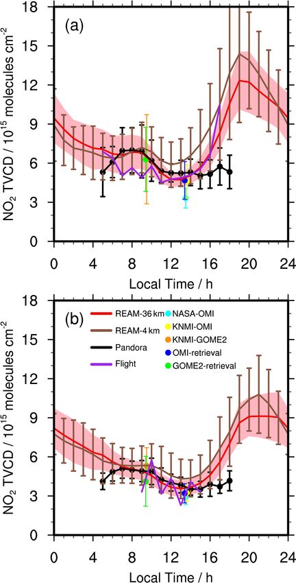
J. Li et al.: Effects of resolution-dependent representation of NOx emissions                                                    11135

                                                                        VCDs, and other physical properties of the atmosphere (An-
                                                                        derson et al., 2014; Reed et al., 2015; Sawamura et al., 2014).
                                                                        Satellite OMI and GOME-2A (Global Ozone Monitoring Ex-
                                                                        periment – 2A) instruments provided NO2 TVCD measure-
                                                                        ments over the campaign region at 13:30 and 09:30 LT, re-
                                                                        spectively. These concurrent measurements of NO2 VCDs,
                                                                        surface NO2 , and vertically resolved distributions of NO2
                                                                        during the DISCOVER-AQ 2011 campaign, therefore, pro-
                                                                        vide a comprehensive dataset to evaluate NO2 diurnal and
                                                                        spatial variabilities and processes affecting NO2 concentra-
                                                                        tions.
                                                                           Section 2 describes the measurement datasets in detail.
                                                                        The Regional chEmistry and trAnsport Model (REAM), also
                                                                        described in Sect. 2, is applied to simulate the NO2 obser-
                                                                        vations during the DISCOVER-AQ campaign in July 2011.
                                                                        The evaluations of the simulated diurnal cycles of surface
                                                                        NO2 concentrations, NO2 vertical profiles, and NO2 TVCDs
                                                                        are discussed in Sect. 3 through comparisons with observa-
                                                                        tions. In Sect. 3, we also investigate the differences between
                                                                        NO2 diurnal cycles on weekdays and weekends and their im-
                                                                        plications for NOx emission characteristics. To corroborate
Figure 1. The locations of surface and P-3B aircraft observations
during the DISCOVER-AQ 2011 campaign. We mark the 36 km                 our evaluation of NOx emissions based on NO2 diurnal cy-
REAM grid cells with red lines and the 4 km REAM grid cells             cles, we further compare observed NOy (reactive nitrogen
with black lines. Gray shading denotes land surface in the nested       compounds) concentrations with REAM simulation results
4 km WRF domain, while the white area denotes ocean or water            in Sect. 3. Moreover, we assess the resolution dependence
surface. Blue dots denote surface O3 observation sites. Cross marks     of REAM simulation results in light of the observations and
denote surface NO2 observation sites, and their colors denote differ-   discuss the potential distribution biases of NOx emissions by
ent measurement instruments: green for the Thermo Electron 42C-         comparing the 36 and 4 km REAM simulation results with
Y NOy analyzer, dark orchid for the Ecotech Model 9841/9843 T-          OMI, GOME-2A, and high-resolution ACAM NO2 VCDs.
NOy analyzers, black for the Thermo Model 42C NOx analyzer,             Finally, we summarize the study in Sect. 4.
and chocolate for the Teledyne API model 200eup photolytic NOx
analyzer. Circles denote Pandora sites, and the cyan circle denotes
a Pandora site (USNA) on a ship. Black squares denote the inland
P-3B aircraft spiral locations.                                         2     Datasets and model description

                                                                        2.1    REAM

access: 6 April 2019), was designed to better understand the            REAM has been widely applied in many studies (Cheng
relationship between boundary layer pollutants and satellite            et al., 2017; Choi et al., 2008; Li et al., 2019; R. Zhang et
observations (Flynn et al., 2014; Reed et al., 2015). Figure 1          al., 2018; Y. Zhang et al., 2016; Zhao et al., 2009). The model
shows the sampling locations of the summer DISCOVER-                    has a horizontal resolution of 36 km and 30 vertical layers
AQ 2011 campaign in the Baltimore–Washington metropoli-                 in the troposphere. Meteorology fields are from a Weather
tan region. In this campaign, the NASA P-3B aircraft flew               Research and Forecasting (WRF; version 3.6) model simu-
spirals over six air quality monitoring sites (Aldino – rural           lation with a horizontal resolution of 36 km. We summarize
and suburban, Edgewood – coastal and urban, Beltsville –                the physics parameterization schemes of the WRF simula-
suburban, Essex – coastal and urban, Fairhill – rural, and              tion in Table S2. The WRF simulation is initialized and con-
Padonia – suburban) (Table S1 in the Supplement) and the                strained by the NCEP coupled forecast system model ver-
Chesapeake Bay (Cheng et al., 2017; Lamsal et al., 2014)                sion 2 (CFSv2) products (http://rda.ucar.edu/datasets/ds094.
and measured 245 NO2 profiles in 14 flight days in July                 0/, last access: 10 March 2015) (Saha et al., 2011). The chem-
(Zhang et al., 2016). During the same period, the NASA UC-              istry mechanism in REAM is based on GEOS-Chem v11.01
12 aircraft flew across the Baltimore–Washington region at              with updated aerosol uptake of isoprene nitrates (Fisher et al.,
an altitude of about 8 km above sea level (a.s.l.), using the           2016) and revised treatment of wet scavenging processes
Airborne Compact Atmospheric Mapper (ACAM) to map                       (Luo et al., 2019). A 2◦ × 2.5◦ GEOS-Chem simulation pro-
the distributions of NO2 VCDs below the aircraft (Lam-                  vides the chemical boundary and initial conditions.
sal et al., 2017). Furthermore, ground-based instruments                   Biogenic VOC emissions in REAM are from MEGAN
were deployed to measure NO2 surface concentrations, NO2                v2.10 (Guenther et al., 2012). Anthropogenic emissions on

https://doi.org/10.5194/acp-21-11133-2021                                              Atmos. Chem. Phys., 21, 11133–11160, 2021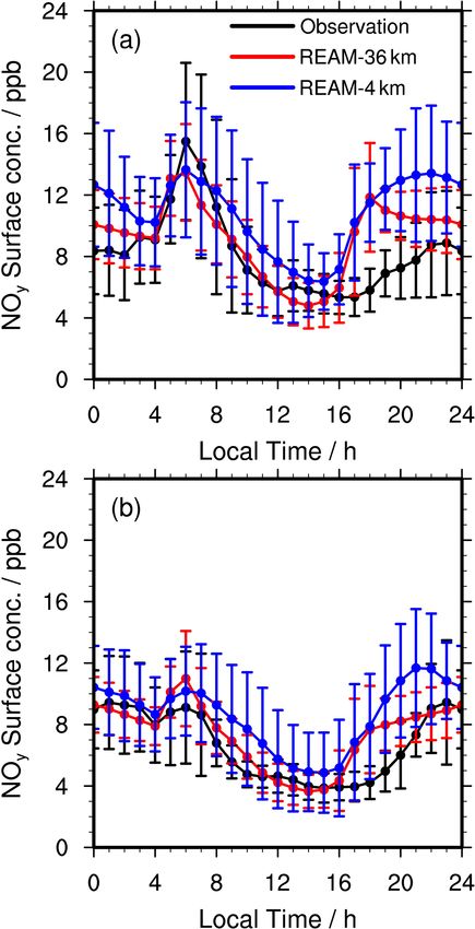
11136                                         J. Li et al.: Effects of resolution-dependent representation of NOx emissions

Figure 2. Distributions of NOx emissions for the (a) 36 km and (b) 4 km REAM simulations around the DISCOVER-AQ 2011 region. Here
NOx emissions refer to the mean values (molecules km−2 s−1 ) in 1 week (Monday–Sunday).

                                                                   than weekday emissions, and the weekend NOx emission
                                                                   diurnal cycles were different from weekdays; therefore, we
                                                                   specify a weekend-to-weekday NOx emission ratio of 2/3 in
                                                                   this study. The resulting diurnal variations in weekday and
                                                                   weekend NOx emissions over the DISCOVER-AQ 2011 re-
                                                                   gion are shown in Fig. 3. The diurnal emission variation is
                                                                   lower on weekends than on weekdays.
                                                                      To understand the effects of model resolutions on the tem-
                                                                   porospatial distributions of NO2 , we also conduct a REAM
                                                                   simulation with a horizontal resolution of 4 km during the
                                                                   DISCOVER-AQ campaign. A 36 km REAM simulation (dis-
                                                                   cussed in Sect. 3.2) provides the chemical initial and hourly
                                                                   boundary conditions. Meteorology fields are from a nested
                                                                   WRF simulation (36, 12, 4 km) with cumulus parameteriza-
Figure 3. Relative diurnal profiles of weekday and weekend NOx
                                                                   tion turned off in the 4 km domain (Table S2). Figure 1 shows
emissions (molecules km−2 s−1 ) in the DISCOVER-AQ 2011 re-
gion (the 36 and 4 km grid cells over the 11 inland Pandora        a comparison of the 4 and 36 km REAM grid cells with
sites shown in Fig. 1) for the 36 and 4 km REAM. All the pro-      DISCOVER-AQ observations, and Fig. 2 shows a compar-
files are scaled by the 4 km weekday emission average value        ison of NOx emission distributions between the 4 and 36 km
(molecules km−2 s−1 ).                                             REAM simulations. The comparison of NOx emission diur-
                                                                   nal variations over the DISCOVER-AQ 2011 region between
                                                                   the 4 and 36 km REAM is shown in Fig. 3.
weekdays are from the National Emission Inventory 2011
(NEI2011) (EPA, 2014) from the Pacific Northwest National          2.2   NO2 TVCD measurements by OMI and GOME-2A
Laboratory (PNNL), which has an initial resolution of 4 km
and is regridded to REAM 36 km grid cells (Fig. 2). Weekday        The OMI instrument onboard the sun-synchronous NASA
emission diurnal profiles are from NEI2011. The weekday-           EOS Aura satellite with an Equator-crossing time of around
to-weekend emission ratios and weekend emission diurnal            13:30 LT was developed by the Finnish Meteorological In-
profiles are based on previous studies (Beirle et al., 2003;       stitute and the Netherlands Agency for Aerospace Programs
Boersma et al., 2009; Choi et al., 2012; de Foy, 2018; Den-        to measure solar backscattering radiation in the visible and
Bleyker et al., 2012; Herman et al., 2009; Judd et al., 2018;      ultraviolet bands (Levelt et al., 2006; Russell et al., 2012).
Kaynak et al., 2009; Kim et al., 2016). These studies sug-         The radiance measurements are used to derive trace gas con-
gested that weekend NOx emissions were 20 %–50 % lower             centrations in the atmosphere, such as O3 , NO2 , HCHO, and

Atmos. Chem. Phys., 21, 11133–11160, 2021                                          https://doi.org/10.5194/acp-21-11133-2021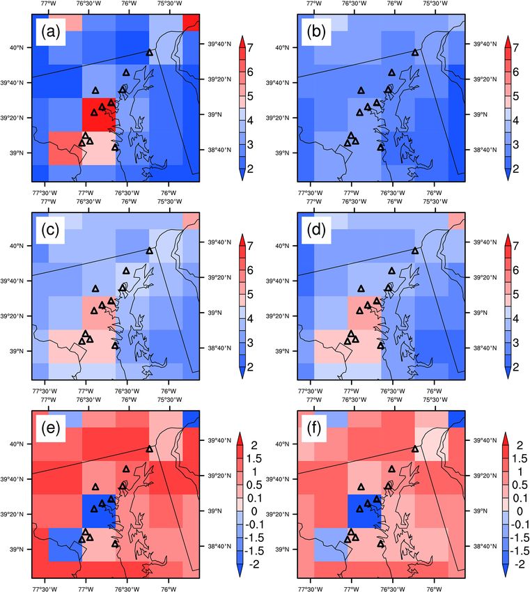
J. Li et al.: Effects of resolution-dependent representation of NOx emissions                                                   11137

SO2 (Levelt et al., 2006). OMI has a nadir resolution of             GOME-2A measures backscattered solar radiation in the
13 km × 24 km and provides daily global coverage (Levelt             range from 240 to 790 nm, which is used for VCD retrievals
et al., 2006).                                                       of trace gases, such as O3 , NO2 , BrO, and SO2 (Munro et al.,
   Two widely used archives of OMI NO2 VCD prod-                     2006). We use the KNMI TM4NO2A v2.3 GOME-2A NO2
ucts are available, NASA OMNO2 (v4.0) (https://disc.                 VCD product archived on http://www.temis.nl/airpollution/
gsfc.nasa.gov/datasets/OMNO2_003/summary, last access:               no2col/no2colgome2_v2.php (last access: 22 January 2015)
26 September 2020) and KNMI DOMINO (v2.0) (https:                    (Boersma et al., 2007, 2011). GOME-2A-derived NO2 VCDs
//www.temis.nl/airpollution/no2.php, last access: 14 January         have been validated with SCIAMACHY and MAX-DOAS
2015). Although both use Differential Optical Absorption             measurements (Irie et al., 2012; Peters et al., 2012; Richter
Spectroscopy (DOAS) algorithms to derive NO2 slant col-              et al., 2011). As in the case of OMI, we use the same criteria
umn densities, they have differences in spectral fitting, strato-    to filter the NO2 TVCD data and recalculate the tropospheric
spheric and tropospheric NO2 slant column density (SCD)              AMF values and GOME-2A TVCDs using the daily 36 km
separation, a priori NO2 vertical profiles, air mass factor          REAM NO2 profiles (09:00–10:00 LT).
(AMF) calculation, etc. (Boersma et al., 2011; Bucsela et al.,
2013; Chance, 2002; Krotkov et al., 2017; Lamsal et al.,             2.3   Pandora ground-based NO2 VCD measurements
2021; Marchenko et al., 2015; Oetjen et al., 2013; van
der A et al., 2010; Van Geffen et al., 2015). Both OMNO2             Pandora is a small direct sun spectrometer which
and DOMINO have been extensively evaluated with field                measures sun and sky radiance from 270 to 530 nm
measurements and models (Boersma et al., 2009, 2011;                 with a 0.5 nm resolution and a 1.6◦ field of view
Choi et al., 2020; Hains et al., 2010; Huijnen et al., 2010;         (FOV) for the retrieval of the total VCDs of NO2
Ionov et al., 2008; Irie et al., 2008; Lamsal et al., 2014,          with a precision of about 5.4 × 10¹⁴ molecules cm−2
2021; Oetjen et al., 2013). The estimated uncertainty in the         (2.7 × 10¹⁴ molecules cm−2 for NO2 SCD) and a nominal
DOMINO TVCD product includes an absolute component of                accuracy of 2.7 × 10¹⁵ molecules cm−2 under clear-sky
1.0 × 10¹⁵ molecules cm−2 and a relative AMF component               conditions (Herman et al., 2009; Lamsal et al., 2014; Zhao
of 25 % (Boersma et al., 2011), while the uncertainty in the         et al., 2020). There were 12 Pandora sites operating in the
OMNO2 TVCD product ranges from ∼ 30 % under clear-                   DISCOVER-AQ campaign (Fig. 1). Six of them are the same
sky conditions to ∼ 60 % under cloudy conditions (Lamsal             as the P-3B aircraft spiral locations (Aldino, Edgewood,
et al., 2014; Oetjen et al., 2013; Tong et al., 2015). In or-        Beltsville, Essex, Fairhill, and Padonia) (Table S1 and
der to reduce uncertainties in this study, we only use TVCD          Fig. 1). The other six sites are Naval Academy (Annapolis,
data with effective cloud fractions < 0.2, solar zenith an-          Maryland) (USNA – ocean), University of Maryland College
gle (SZA) < 80◦ , and albedo ≤ 0.3. Both positive and neg-           Park (UMCP – urban), University of Maryland Baltimore
ative TVCDs are considered in the calculation. The data af-          County (UMBC – urban), Smithsonian Environmental
fected by row anomaly are excluded (Boersma et al., 2018;            Research Center (SERC – rural and coastal), Oldtown in
R. Zhang et al., 2018).                                              Baltimore (Oldtown – urban), and Goddard Space Flight
   For AMF calculation, DOMINO used daily TM4 model                  Center (GSFC – urban and suburban) (Table S1 and Fig. 1).
results with a resolution of 3◦ × 2◦ as a priori NO2 vertical        In this study, we exclude the USNA site as its measurements
profiles (Boersma et al., 2007, 2011), while OMNO2 v4.0              were conducted on a ship (“Pandora(w)” in Fig. 1), and there
used monthly mean values from the Global Modeling Initia-            were no other surface observations in the corresponding
tive (GMI) model with a resolution of 1◦ × 1.25◦ . The rel-          REAM grid cell. Including the data from the USNA site
atively coarse horizontal resolution of the a priori NO2 pro-        has a negligible effect on the comparisons of observed
files in the retrievals can introduce uncertainties in the spatial   and simulated NO2 TVCDs. In our analysis, we ignore
and temporal characteristics of NO2 TVCDs at satellite pixel         Pandora measurements with SZA > 80◦ (Fig. S1 in the
scales. For comparison purposes, we also use 36 km REAM              Supplement) and exclude the data when fewer than three
simulation results as the a priori NO2 profiles to compute the       valid measurements are available within an hour to reduce
AMFs and NO2 TVCDs with the DOMINO algorithm. The                    the uncertainties in the hourly averages due to the significant
36 km REAM NO2 data are first regridded to OMI pixels to             variations in Pandora observations (Fig. S2).
calculate the corresponding tropospheric AMFs, which are                Since Pandora measures total NO2 VCDs, we need to sub-
then applied to compute OMI NO2 TVCDs by dividing the                tract stratosphere NO2 VCDs from the total VCDs to com-
tropospheric SCDs from the DOMINO product by our up-                 pute TVCDs. As shown in Fig. S3, stratosphere NO2 VCDs
dated AMFs.                                                          show a clear diurnal cycle with an increase during daytime
   The GOME-2 instrument onboard the polar-orbiting                  due in part to the photolysis of reactive nitrogen reservoirs
MetOp-A satellite (now referred to as GOME-2A) is an                 such as N2 O5 and HNO3 (Brohede et al., 2007; Dirksen et al.,
improved version of GOME-1 launched in 1995 and has                  2011; Peters et al., 2012; Sen et al., 1998; Spinei et al., 2014),
an overpass time of 09:30 LT and a spatial resolution of             which is consistent with the significant increase in strato-
80 km × 40 km (Munro et al., 2006; Peters et al., 2012).             spheric NO2 VCDs from GOME-2A to OMI. In this study,

https://doi.org/10.5194/acp-21-11133-2021                                           Atmos. Chem. Phys., 21, 11133–11160, 2021
11138                                          J. Li et al.: Effects of resolution-dependent representation of NOx emissions

we use the GMI model-simulated stratospheric NO2 VCDs             which are then used to evaluate the distribution of NO2
in Fig. S3 to calculate the Pandora NO2 TVCDs. The small          VCDs in the 4 km REAM simulation. As a supplement in
discrepancies between the GMI stratospheric NO2 VCDs and          Sect. 3.7, we also assess the 4 km REAM simulation by us-
satellite products do not change the pattern of Pandora NO2       ing the UC-12 ACAM NO2 VCDs produced by the Smithso-
TVCD diurnal variations or affect the conclusions in this         nian Astrophysical Observatory (SAO) algorithms, archived
study.                                                            on https://www-air.larc.nasa.gov/cgi-bin/ArcView/discover-
                                                                  aq.dc-2011?UC12=1#LIU.XIONG/ (last access: December
2.4   ACAM NO2 VCD measurements                                   31, 2019) (Liu et al., 2015a, b). This product is an early ver-
                                                                  sion of the SAO algorithm used to produce the Geostationary
The ACAM instrument onboard the UC-12 aircraft consists           Trace gas and Aerosol Sensor Optimization (GeoTASO) and
of two thermally stabilized spectrometers in the ultraviolet,     the GEOstationary Coastal and Air Pollution Events (GEO-
visible, and near-infrared range. The spectrometer in the ul-     CAPE) Airborne Simulator (GCAS) airborne observations in
traviolet and visible band (304–520 nm) with a resolution of      later airborne campaigns (Nowlan et al., 2016, 2018).
0.8 nm and a sampling of 0.105 nm can be used to detect NO2
in the atmosphere. The native ground resolution of UC-12          2.5   Surface NO2 and O3 measurements
ACAM NO2 measurements is 0.5 km × 0.75 km at a flight
altitude of about 8 km a.s.l. and a nominal ground speed of       The measurement of NOx is based on the chemiluminescence
100 m s−1 during the DISCOVER-AQ 2011 campaign (Lam-              of electronically excited NO∗2 , produced from the reaction of
sal et al., 2017), thus providing high-resolution NO2 VCDs        NO with O3 , and the strength of the chemiluminescence from
below the aircraft.                                               the decay of NO∗2 to NO2 is proportional to the number of NO
   In this study, we mainly use the ACAM NO2 VCD prod-            molecules present (Reed et al., 2016). NO2 concentrations
uct described by Lamsal et al. (2017), which applied a            can be measured with this method by converting NO2 to NO
pair-average co-adding scheme to produce NO2 VCDs at              first through catalytic reactions (typically on the surface of
a ground resolution of about 1.5 km (cross-track) × 1.1 km        heated molybdenum oxide (MoOx ) substrate) or photolytic
(along-track) to reduce noise impacts. In their retrieval of      processes (Lamsal et al., 2015; Reed et al., 2016). However,
ACAM NO2 VCDs, they first used the DOAS fitting method            for the catalytic method, reactive nitrogen compounds other
to generate differential NO2 SCDs relative to the SCDs at an      than NOx (NOz ), such as HNO3 , peroxyacetyl nitrate (PAN),
unpolluted reference location. Then they computed above-          and other organic nitrates, can also be reduced to NO on the
and below-aircraft AMFs at both sampling and reference lo-        heated surface, thus causing an overestimation of NO2 . The
cations based on the vector linearized discrete ordinate radia-   magnitude of the overestimation depends on the concentra-
tive transfer code (VLIDORT) (Spurr, 2008). In the computa-       tions and the reduction efficiencies of interference species,
tion of AMFs, the a priori NO2 vertical profiles were from a      both of which are uncertain. The photolytic approach, which
combination of high-resolution (4 km) CMAQ (the Commu-            employs broadband photolysis of ambient NO2 , offers more
nity Multiscale Air Quality Modeling System) model outputs        accurate NO2 measurements (Lamsal et al., 2015).
in the boundary layer and GMI simulation (2◦ × 2.5◦ ) results        There were 11 NOx monitoring sites operating in the
elsewhere in the atmosphere. Finally, the below-aircraft NO2      DISCOVER-AQ region during the campaign (Fig. 1), includ-
VCDs at the sampling locations were generated by divid-           ing those from the EPA Air Quality System (AQS) moni-
ing below-aircraft NO2 SCDs at the sampling locations by          toring network and those deployed for the DISCOVER-AQ
the corresponding below-aircraft AMFs. The below-aircraft         campaign. Nine of them measured NO2 concentrations by a
NO2 SCDs were the differences between the total and above-        catalytic converter. The other two sites (Edgewood and Pado-
aircraft NO2 SCDs. The total NO2 SCDs were the sum                nia) had NO2 measurements from both catalytic and pho-
of DOAS-fitting-generated differential NO2 SCDs and NO2           tolytic methods. Different stationary catalytic instruments
SCDs at the reference location, and the above-aircraft NO2        were used during the campaign: Thermo Electron 42C-Y
SCDs were derived based on above-aircraft AMFs, GMI               NOy analyzer, Thermo Model 42C NOx analyzer, Thermo
NO2 profiles, and OMNO2 stratospheric NO2 VCDs (Lam-              Model 42I-Y NOy analyzer, and Ecotech Model 9843 and
sal et al., 2017). The ACAM NO2 VCD product had been              9841 T-NOy analyzers. In addition, a mobile platform – NA-
evaluated via comparisons with other independent observa-         TIVE (Nittany Atmospheric Trailer and Integrated Validation
tions during the DISCOVER-AQ 2011 campaign, such as P-            Experiment) with a Thermo Electron 42C-Y NOy analyzer
3B aircraft, Pandora, and OMNO2, and the uncertainty in           installed – was also deployed at the Edgewood site. The pho-
individual below-aircraft NO2 VCD is about 30 % (Lam-             tolytic measurements of NO2 in Edgewood and Padonia were
sal et al., 2017). To keep the consistency of ACAM NO2            from Teledyne API model 200eup photolytic NOx analyzers.
VCDs, we exclude NO2 VCDs measured at altitudes <                 We scale catalytic NO2 measurements using the diurnal ra-
8 km a.s.l., which accounts for about 6.8 % of the total avail-   tios of NO2 photolytic measurements to NO2 from the cor-
able ACAM NO2 VCD data. We regrid the 1.5 km × 1.1 km             responding catalytic analyzers (Fig. 4). Figure 4 shows the
ACAM NO2 VCDs to the 4 km REAM grid cells (Fig. 1),               lowest photolytic–catalytic ratio in the afternoon, which re-

Atmos. Chem. Phys., 21, 11133–11160, 2021                                         https://doi.org/10.5194/acp-21-11133-2021
J. Li et al.: Effects of resolution-dependent representation of NOx emissions                                               11139

                                                                   in the daytime for July 2011 are used to compute the average
                                                                   profiles of NO2 for the six inland sites (Fig. 1).
                                                                      The aircraft measurements were generally sampled from
                                                                   a height of about 300 m a.g.l. (above ground level) in the
                                                                   boundary layer to 3.63 km a.g.l. in the free troposphere. We
                                                                   bin these measurements to REAM vertical levels. In order to
                                                                   make up the missing observations between the surface and
                                                                   300 m, we apply quadratic polynomial regressions by using
                                                                   aircraft data below 1 km and coincident NO2 surface mea-
                                                                   surements.
                                                                      In addition to using NO2 concentrations from the NCAR
                                                                   four-channel instrument to evaluate REAM-simulated NO2
                                                                   vertical profiles, we also use P-3B NO, NO2 , and NOy con-
                                                                   centrations measured by the NCAR four-channel        instrument
Figure 4. Hourly ratios of NO2 measurements from the Teledyne                                              P
                                                                   and NO   2 , total peroxyacyl nitrates (  PNs),  total alkyl ni-
API model 200 eup photolytic NOx analyzer to NO2 from coinci-              P
dent catalytic instruments for 2011 July. “CY42” denotes the ra-   trates ( ANs) (including alkyl nitrates and hydroxyalkyl ni-
tios of photolytic NO2 to NO2 from the Thermo Electron 42C-Y       trates), and HNO3 concentrations measured by the thermal-
NOy analyzer in Edgewood, “C42” denotes the ratios of photolytic   dissociation laser-induced fluorescence (TD-LIF) technique
NO2 to NO2 from the Thermo Model 42C NOx analyzer in Pado-         (Day et al., 2002; Thornton et al., 2000; Wooldridge et al.,
nia, and “ECO” denotes the ratios of photolytic NO2 to NO2 from    2010) to evaluate the concentrations of NOy from REAM
the Ecotech Model 9841 T-NOy analyzer in Padonia. “ECO” ratios     (Table 1). All these P-3B measurements are vertically binned
are also used to scale NO2 measurements from the Ecotech Model     to REAM grid cells for comparisons with REAM results. In
9843 T-NOy analyzer.                                               addition, below the P-3B spirals, four NOy observation sites
                                                                   at Padonia, Edgewood, Beltsville, and Aldino were operat-
                                                                   ing to provide continuous hourly NOy surface concentrations
                                                                   during the campaign, which we also use to evaluate REAM-
flects the production of nitrates and other reactive nitrogen
                                                                   simulated NOy surface concentrations in this study. We sum-
compounds from NOx in the daytime. When photolytic mea-
                                                                   marize the information of available observations at the 11 in-
surements are available, we only use the photolytic obser-
                                                                   land Pandora sites in Table S1.
vations in this study; otherwise, we use the scaled catalytic
measurements.
   Nineteen surface O3 monitoring sites were operating in
the DISCOVER-AQ region during the campaign (Fig. 1).               3     Results and discussion
They measured O3 concentrations by using a federal equiv-
                                                                   3.1    Evaluation of WRF-simulated meteorological fields
alent method (FEM) based on the UV absorption of O3
(https://cfpub.epa.gov/si/si_public_file_download.cfm?p_
                                                                   We evaluate the performances of the 36 km and nested
download_id=520887&Lab=NERL, last access: 12 July
                                                                   4 km WRF simulations using temperature, potential tem-
2021) with an uncertainty of 5 ppb.
                                                                   perature, relative humidity (RH), and wind measurements
                                                                   from the P-3B spirals (Fig. 1) and precipitation data from
2.6   Aircraft measurements of NO2 vertical profiles               the NCEP (National Centers for Environmental Predic-
                                                                   tion) Stage IV precipitation dataset. Generally, P-3B spi-
In this study, we mainly use the NO2 concentrations mea-           rals range from ∼ 300 m to ∼ 3.63 km in height above the
sured by the National Center for Atmospheric Research              ground level (a.g.l.). As shown in Fig. S4, both the 36 km
(NCAR) four-channel chemiluminescence instrument (P-               and nested 4 km WRF simulations simulate temperature
CL) onboard the P-3B aircraft for the evaluation of REAM-          well with R 2 = 0.98. Both WRF simulations show good
simulated NO2 vertical profiles. The instrument has an NO2         agreement with P-3B measurements in U wind (36 km:
measurement uncertainty of 10 %–15 % and a 1 s, 1σ detec-          R 2 = 0.77; 4 km: R 2 = 0.76), V wind (36 km: R 2 = 0.79;
tion limit of 30 pptv.                                             4 km: R 2 = 0.78), wind speed (36 km: R 2 = 0.67; 4 km:
   NO2 measurements from aircraft spirals provide us with          R 2 = 0.67), and wind direction (Figs. S4 and S5). We fur-
NO2 vertical profiles. Figure 1 shows the locations of the         ther compare the temporal evolutions of vertical profiles for
aircraft spirals during the DISCOVER-AQ campaign, except           temperature, potential temperature, RH, U wind, and V wind
for the Chesapeake Bay spirals over the ocean. There were          below 3 km from the P-3B observations with those from the
only six spirals available over the Chesapeake Bay, which          36 km and nested 4 km WRF simulations in Fig. S6. Both
have ignorable impacts on the following analyses. Therefore,       WRF simulations capture the temporospatial variations in
we do not use them in this study. The remaining 239 spirals        P-3B-observed vertical profiles well except that RH below

https://doi.org/10.5194/acp-21-11133-2021                                         Atmos. Chem. Phys., 21, 11133–11160, 2021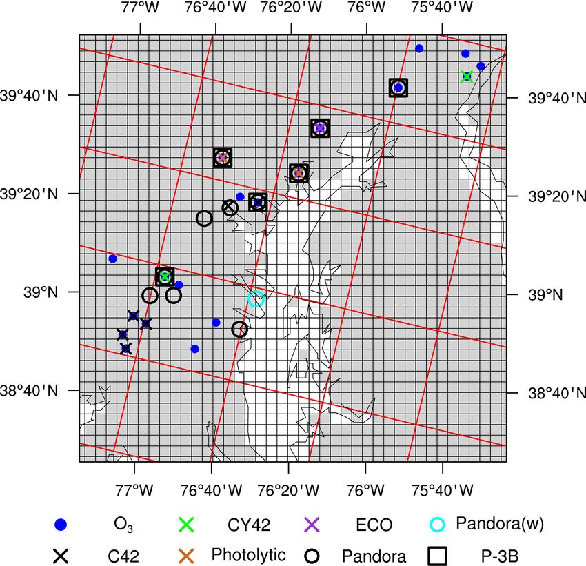
J. Li et al.: Effects of resolution-dependent representation of NOx emissions
https://doi.org/10.5194/acp-21-11133-2021
Table 1. Comparison of the concentrations of NOy and its components between REAM and P-3B aircraft measurements during the DISCOVER-AQ campaign.
NOy (ppb1 ) NO2 _LIF (ppb2 ) Derived-NOy (ppb3 )
P P
NO (ppb) NO2 _NCAR (ppb) PNs (ppb) ANs (ppb) HNO3 (ppb)
36 km4 Weekday5 P-3B 2.51 ± 2.09 0.18 ± 0.29 0.85 ± 1.13 0.68 ± 0.95 0.70 ± 0.58 0.31 ± 0.23 1.15 ± 0.73 2.86 ± 2.26
REAM 3.64 ± 3.13 0.18 ± 0.30 0.74 ± 1.04 0.68 ± 0.89 0.54 ± 0.45 0.10 ± 0.09 1.80 ± 1.61 3.10 ± 2.70
R2 0.33 0.35 0.38 0.34 0.37 0.38 0.24 0.41
Weekend P-3B 3.00 ± 2.18 0.15 ± 0.20 0.71 ± 0.80 0.63 ± 0.72 0.91 ± 0.53 0.36 ± 0.21 1.15 ± 0.79 2.96 ± 2.15
REAM 3.78 ± 2.20 0.15 ± 0.17 0.54 ± 0.59 0.53 ± 0.58 0.53 ± 0.29 0.09 ± 0.06 2.31 ± 1.38 3.43 ± 2.26
R2 0.29 0.28 0.41 0.45 0.27 0.39 0.50 0.51
4 km Weekday P-3B 2.51 ± 2.15 0.19 ± 0.30 0.86 ± 1.27 0.68 ± 0.98 0.70 ± 0.59 0.31 ± 0.22 1.17 ± 0.74 2.90 ± 2.27
REAM 3.81 ± 3.81 0.19 ± 0.35 0.79 ± 1.31 0.76 ± 1.20 0.46 ± 0.51 0.08 ± 0.10 2.03 ± 1.91 3.31 ± 3.28
R2 0.28 0.22 0.26 0.32 0.37 0.29 0.38 0.47
Weekend P-3B 2.96 ± 2.13 0.14 ± 0.18 0.69 ± 0.74 0.63 ± 0.71 0.91 ± 0.51 0.35 ± 0.21 1.15 ± 0.80 2.94 ± 2.09
REAM 4.36 ± 3.66 0.25 ± 0.40 0.85 ± 1.28 0.81 ± 1.23 0.41 ± 0.29 0.08 ± 0.08 2.54 ± 1.99 3.72 ± 3.52
R2 0.21 0.15 0.19 0.18 0.16 0.23 0.38 0.37
1 For P-3B, the concentrations of NO , NO, and NO _NCAR were measured by using the NCAR four-channel chemiluminescence instrument. The measurement uncertainties are 10 %, 10 %–15 %, and 10 % for NO, NO , and NO ,
y 2 2 y
respectively. The 1 s, 1σ detection limits are 20, 30, and 20 pptv for NO, NO2 , and NOy , respectively
P (https://discover-aq.larc.nasa.gov/wp-content/uploads/sites/140/2020/05/Weinheimer20101005_DISCOVERAQ_AJW.pdf,
P last
access: 28 June 2019). For REAM, NOy is the sum of NO, NO2 , total peroxyacyl nitrates ( PNs), total alkyl nitrates ( ANs) (including alkyl nitrates and hydroxyalkyl nitrates), HNO3 , HONO, 2 × N2 O5 , HNO4 , first-generation
Atmos. Chem. Phys., 21, 11133–11160, 2021
C5 carbonyl nitrate (nighttime isoprene nitrate ISN1: C5 H8 NO4 ), 2 × C5 dihydroxy dinitrate (DHDN: C5 H10 O8 N2 ), methyl peroxy nitrate (MPN: CH3 O2 NO2 ), propanone nitrate (PROPNN: CH3 C(=O)CH2 ONO2 ), nitrate from
methyl vinyl ketone (MVKN: HOCH2 CH(ONO2 )C(=O)CH3 ), nitrate from methacrolein (MARCN: HOCH2 C(ONO2 )(CH3 )CHO), and ethanol nitrate (ETHLN: CHOCH2 ONO2 ).
2 For P-3B, the concentrations of NO _LIF, P PNs, P ANs, and HNO were measured by applying the thermal-dissociation laser-induced fluorescence (TD-LIF) technique. The accuracy of TD-LIF measurements of NO , P PNs,
2 3 2
ANs, and HNO3 is better than 15 %, and the detection limit for the sum of NO2 , PNs, ANs, and HNO3 is ∼ 10 ppt 10 s−1 (Day et al., 2002).
P P P
3 To compare NO concentrations from TD-LIF measurements with those from REAM, we calculate derived-NO as the sum of NO, NO _LIF, P PNs, P ANs, and HNO . Only when the concentrations of all the five species are
y y 2 3
availablePat the same hour in the same grid cell can we calculate derived-NOy at the given hour in the given grid cell. Therefore, in Table 1, the averaged derived-NOy values are not exactly equal to the sum of averaged NO, NO2 _LIF,
P
PNs, ANs, and HNO3 concentrations that only depend on the availability of a single species. In addition, the measurement times and frequencies between NOy and derived-NOy are not the same. A comparison between these two
types of data needs coincident sampling, as described in the main text.
4 Mean NO emissions over the six P-3B spiral sites are close (relative difference < 4 %) between the 36 and 4 km REAM (Table S1).
x
5 Due to different sampling times and locations between weekdays and weekends, we do not recommend a direct comparison between weekday and weekend values here.
11140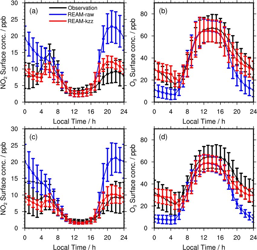
J. Li et al.: Effects of resolution-dependent representation of NOx emissions 11141
1.5 km is significantly underestimated between 09:00 and
17:00 LT in both WRF simulations. The evaluations above
suggest that WRF-simulated wind fields are good and com-
parable at 4 and 36 km resolutions, but potential dry biases
exist in both WRF simulations.
The NCEP Stage IV precipitation dataset provides hourly
precipitation across the contiguous United States (CONUS)
with a resolution of ∼ 4 km based on the merging of rain
gauge data and radar observations (Lin and Mitchell, 2005;
Nelson et al., 2016). The Stage IV dataset is useful for eval-
uating model simulations, satellite precipitation estimates,
and radar precipitation estimates (Davis et al., 2006; Gour-
ley et al., 2011; Kalinga and Gan, 2010; Lopez, 2011;
Yuan et al., 2008). We obtain the Stage IV precipitation
data for July 2011 from the NCAR/UCAR Research Data
Archive (https://rda.ucar.edu/datasets/ds507.5/, last access:
28 December 2019). As shown in Figs. S7 and S8, both the
36 km and nested 4 km WRF simulations generally predict
much less precipitation (in precipitation amount and dura-
tion) compared to the Stage IV data in July 2011 around the
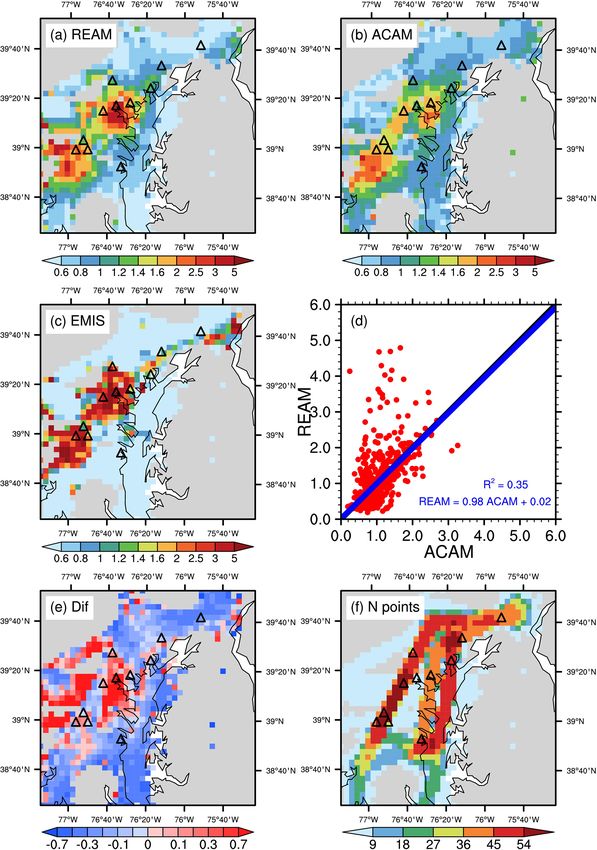
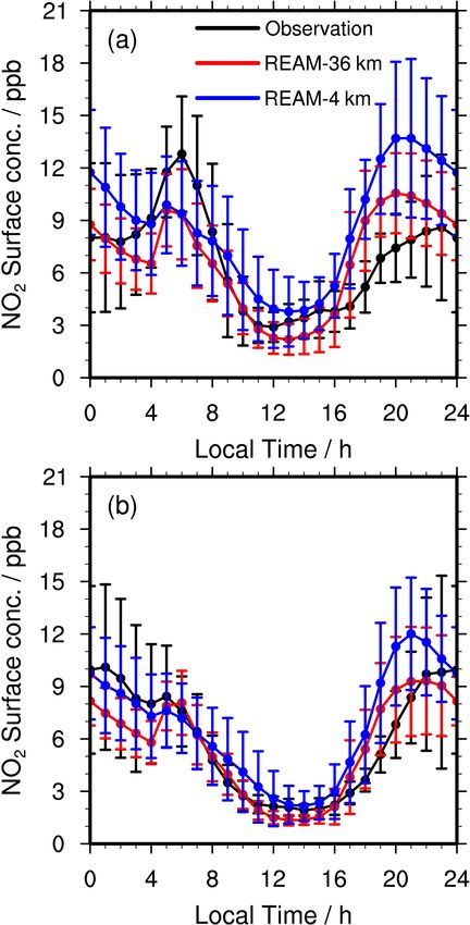
DISCOVER-AQ campaign region, especially for the nested Figure 5. Diurnal cycles of surface (a, c) NO2 and (b, d) O3
4 km WRF simulation, consistent with the aforementioned concentrations on (a, b) weekdays and (c, d) weekends during
underestimated RH and dry bias in WRF simulations. The the DISCOVER-AQ campaign in the DISCOVER-AQ region (the
precipitation biases in the WRF model will affect REAM 36 km grid cells over the 11 inland Pandora sites shown in Fig. 1).
simulations of trace gases, leading to high biases of soluble Black lines denote the mean observations from all the 11 NO2 sur-
species due to underestimated wet scavenging. Clouds inter- face monitoring sites and 19 O3 surface sites during the campaign
(Fig. 1), as mentioned in Sect. 2.5. “REAM-raw” (blue lines) de-
fere with satellite observations. Therefore, the precipitation
notes the coincident 36 km REAM simulation results with WRF-
bias does not affect model evaluations with satellite mea-
YSU-simulated kzz data, and “REAM-kzz” (red lines) is the coin-
surements of NO2 . Aircraft measurements were also taken cident 36 km REAM simulation results with updated kzz data. See
on non-precipitating days. the main text for details. Vertical bars denote corresponding stan-
dard deviations.
3.2 Effect of boundary layer vertical mixing on the
diurnal variations in surface NO2 concentrations
biases with WRF-YSU-simulated kzz data in Fig. 5 indicate
that vertical mixing may be underestimated at night.
3.2.1 36 km model simulation in comparison to the During the DISCOVER-AQ campaign, WRF-simulated
surface observations vertical wind velocities are very low at night and have lit-
tle impact on vertical mixing (Fig. S9a). The nighttime ver-
Figure 5a and b show the observed and 36 km REAM- tical mixing is mainly attributed to turbulent mixing. How-
simulated diurnal cycles of surface NO2 and O3 concen- ever, Hu et al. (2012) found that the YSU scheme un-
trations on weekdays in July 2011 in the DISCOVER-AQ derestimated nighttime PBL vertical turbulent mixing in
region. REAM with WRF-YSU-simulated vertical diffusion WRF, which is consistent with Fig. 6, showing that WRF-
coefficient (kzz ) values significantly overestimates NO2 con- YSU kzz -determined mixed-layer heights (MLHs) are sig-
centrations and underestimates O3 concentrations at night, nificantly lower than lidar observations in the late afternoon
although it captures the patterns of the diurnal cycles of sur- and at night at the UMBC site during the DISCOVER-AQ
face NO2 and O3 : an O3 peak and an NO2 minimum around campaign (Knepp et al., 2017). Here, the kzz -determined
noontime. Here, YSU denotes the Yonsei University plane- MLH refers to the mixing height derived by comparing kzz
tary boundary layer (PBL) scheme (Shin and Hong, 2011) to its background values (Hong et al., 2006) but not the
used by our WRF simulations (Table S2). At night, the re- PBLH outputs from WRF. UMBC is an urban site (Ta-
action of O3 + NO → O2 + NO2 produces NO2 but removes ble S1), surrounded by a mixture of constructed materials
O3 . Since most NOx emissions are in the form of NO, the and vegetation. The UMBC lidar MLH data were derived
model biases of low O3 and high NO2 occur at the same time. from the Elastic Lidar Facility (ELF) attenuated backscat-
Since there are no significant chemical sources of O3 at night, ter signals by using the covariance wavelet transform (CWT)
mixing of O3 -rich air above the surface is the main source of method and had been validated against radiosonde mea-
O3 supply near the surface. Therefore, the nighttime model surements (N (number of data points) = 24; R 2 = 0.89; bias
https://doi.org/10.5194/acp-21-11133-2021 Atmos. Chem. Phys., 21, 11133–11160, 2021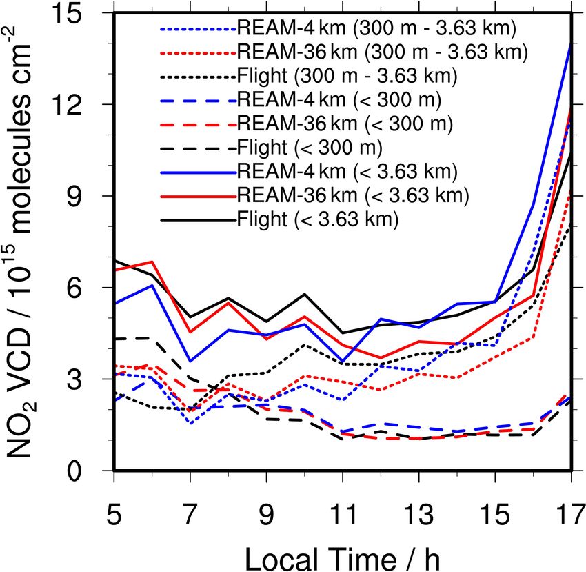
11142                                            J. Li et al.: Effects of resolution-dependent representation of NOx emissions

                                                                     Virginia (Knepp et al., 2017). Finally, we want to emphasize
                                                                     that different definitions of NBL can result in significantly
                                                                     different NBL heights (Breuer et al., 2014). In this study, we
                                                                     follow Knepp et al. (2017) to use MLHs derived from aerosol
                                                                     backscatter signals as the measure of vertical pollutant mix-
                                                                     ing within the boundary layer, which is simulated by kzz in
                                                                     REAM.
                                                                        To improve nighttime PBL vertical turbulent mixing
                                                                     in REAM, we increase kzz below 500 m between 18:00
                                                                     and 05:00 LT to 5 m s−2 if the WRF-YSU-computed
                                                                     kzz < 5 m s−2 , which significantly increases the kzz -
                                                                     determined MLHs at night (Fig. 6), leading to the decreases
                                                                     in simulated surface NO2 and the increases in surface O3
                                                                     concentrations at night (Fig. 5). The assigned value of
Figure 6. ELF-observed and model-simulated diurnal variations in
MLH at the UMBC site during the Discover-AQ campaign. “ELF           5 m s−2 is arbitrary. Changing this value to 2 or 10 m s−2
MLH” denotes ELF-derived MLHs by using the covariance wavelet        can also alleviate the biases of model-simulated nighttime
transform method. “WRF-YSU MLH” denotes the 36 km WRF-               surface NO2 and O3 concentrations (Fig. S10). Considering
YSU kzz -determined MLHs, and “Updated MLH” denotes updated          the potential uncertainties in nighttime NOx emissions, an
kzz -determined MLHs. See the main text for details. Vertical bars   alternative solution to correct the model nighttime simulation
denote standard deviations. For the ELF MLHs, there are 13 506       biases is to reduce NOx emissions, which can decrease the
1 min measurements in total during the campaign, and we bin them     consumption of O3 through the process of NOx titration
into hourly data. The green line corresponding to the right y axis   mentioned above (O3 + NO → O2 + NO2 ). Our sensitivity
shows the diurnal variations in the number of hourly ELF data        tests (not shown) indicate that it is necessary to reduce NOx
points.
                                                                     emissions by 50 %–67 % to eliminate the model nighttime
                                                                     simulation biases, but we cannot find good reasons to justify
                                                                     this level of NOx emission reduction only at night.
(ELF – radiosonde) = 0.03 ± 0.23 km), radar wind profiler               The updated REAM simulation of surface NO2 diurnal
observations (N = 659; R 2 = 0.78; bias = −0.21 ± 0.36 km),          pattern in Fig. 5a is in good agreement with previous stud-
and Sigma Space mini-micropulse lidar data (N = 8122;                ies (Anderson et al., 2014; David and Nair, 2011; Gaur et al.,
R 2 = 0.85; bias = 0.02 ± 0.22 km) from the Howard Univer-           2014; Reddy et al., 2012; Zhao et al., 2019). Daytime surface
sity Beltsville Research Campus (HUBRC) in Beltsville,               NO2 concentrations are much lower compared to nighttime,
Maryland (38.058◦ N, 76.888◦ W) in the daytime during                and NO2 concentrations reach a minimum around noontime.
the DISCOVER-AQ campaign (Compton et al., 2013). It                  As shown in Fig. S11, under the influence of vertical turbu-
is noteworthy that although CWT is not designed to detect            lent mixing, the surface layer NOx emission diurnal pattern
the nocturnal boundary layer (NBL), it does consider the             is similar to the surface NO2 diurnal cycle in Fig. 5a, em-
residue layer (RL) and distinguish it from MLH in the early          phasizing the importance of turbulent mixing on modulating
morning after sunrise, which is similar to nighttime condi-          surface NO2 diurnal variations. The highest boundary layer
tions. Therefore, CWT can detect nighttime MLHs, although            (Fig. 6) due to solar radiation leads to the lowest surface layer
with large uncertainties due to the hard-coded assumption of         NOx emissions (Fig. S11), and, therefore, the smallest sur-
RL = 1 km in the algorithm and insufficient vertical resolu-         face NO2 concentrations occur around noontime (Fig. 5a).
tion of the technique. In addition, the sunrise and sunset time      Transport, which is mainly attributed to advection and turbu-
in July 2011 is about 05:00 and 19:30 LT (https://gml.noaa.          lent mixing, is another critical factor affecting surface NO2
gov/grad/solcalc/sunrise.html, last access: 27 May 2021), re-        diurnal variations (Fig. S11). The magnitudes of transport
spectively. Figure 6 shows that WRF-YSU kzz -determined              fluxes (Fig. S11) are proportional to horizontal and vertical
MLHs are significantly lower than ELF observations after             gradients of NOx concentrations and are therefore generally
sunrise between 05:00 and 08:00 LT and before sunset be-             positively correlated to surface NO2 concentrations. How-
tween 18:00 and 20:00 LT. Even if we do not consider MLHs            ever, some exceptions exist, reflecting different strengths of
at night (19:30–05:00 LT), we can still conclude that WRF-           advection (U , V , and W ) and turbulent mixing (kzz ) at dif-
YSU underestimates vertical mixing in the early morning af-          ferent times. For example, in the early morning, NO2 surface
ter sunrise and the late afternoon before sunset, enabling a         concentrations peak between 05:00 and 06:00 LT (Fig. 5a),
reasonable assumption that WRF-YSU also underestimates               while transport fluxes peak between 07:00 and 08:00 LT
nighttime vertical mixing. Moreover, the nighttime MLHs in           (Fig. S11). The delay of the peak is mainly due to lower tur-
Fig. 6 are comparable to those measured by the Vaisala CL51          bulent mixing between 05:00 and 06:00 LT than other day-
ceilometer at the Chemistry And Physics of the Atmospheric           time hours in the model (Fig. 6). Chemistry also contributes
Boundary Layer Experiment (CAPABLE) site in Hampton,                 to surface NO2 diurnal variations mainly through photo-

Atmos. Chem. Phys., 21, 11133–11160, 2021                                            https://doi.org/10.5194/acp-21-11133-2021
J. Li et al.: Effects of resolution-dependent representation of NOx emissions 11143
chemical sinks in the daytime and N2 O5 hydrolysis at night-
time. Chemistry fluxes in Fig. S11 are not only correlated to
the strength of photochemical reactions and N2 O5 hydrolysis
(chemistry fluxes per unit NOx ) but are also proportional to
NOx surface concentrations. Therefore, chemistry fluxes in
Fig. S11 cannot directly reflect the impact of solar radiation
on photochemical reactions. It can, however, still be identi-
fied by comparing afternoon chemistry contributions: from
13:00 to 15:00 LT, surface layer NOx emissions and NO2
concentrations are increasing (Figs. S11 and 5a); however,
chemistry losses are decreasing as a result of the reduction
in photochemical sinks with weakening solar radiation. The
contributions of vertical mixing and photochemical sinks to
NO2 concentrations can be further corroborated by daytime
variations in NO2 vertical profiles and TVCDs discussed in
Sects. 3.3 and 3.4.
Figure 5c shows the diurnal variation on weekends is
also simulated well in the improved 36 km model. The di-
urnal variation in surface NO2 concentrations (REAM: 1.5–
10.2 ppb; observations: 2.1–9.8 ppb) is lower than on week-
days (REAM: 2.4–12.2 ppb; observations: 3.3–14.5 ppb), re-
flecting lower magnitude and variation in NOx emissions on
weekends (Fig. 3). Figure 5d also shows an improved sim-
ulation of surface O3 concentrations at nighttime due to the
improved MLH simulation (Fig. 6).
Figure 7. Diurnal cycles of observed and simulated average sur-
3.2.2 4 km model simulation in comparison to the face NO2 concentrations over Padonia, Oldtown, Essex, Edgewood,
surface observations Beltsville, and Aldino (Table S1) on (a) weekdays and (b) week-
ends. Black lines denote mean observations from the six sites. Red
lines denote coincident 36 km REAM simulation results, and blue
The results of 4 km REAM simulations with original WRF- lines are for coincident 4 km REAM simulation results. Error bars
YSU kzz (not shown) are very similar to Fig. 5 since WRF- denote standard deviations.
simulated nocturnal vertical mixing is insensitive to the
model horizontal resolution. Applying the modified noctur-
nal mixing in the previous section also greatly reduced the 3.3 Diurnal variations in NO2 vertical profiles
nighttime NO2 overestimate and O3 underestimate in the
4 km REAM simulations. All the following analyses are Figure 8a and c show the temporal variations in P-3B-
based on REAM simulations with improved nocturnal mix- observed and 36 km REAM-simulated NO2 vertical pro-
ing. Figure 7 shows that mean surface NO2 concentrations files in the daytime on weekdays during the DISCOVER-
simulated in the 4 km model are higher than the 36 km re- AQ campaign. The 36 km REAM reproduces the observed
sults over Padonia, Oldtown, Essex, Edgewood, Beltsville, characteristics of NO2 vertical profiles well in the daytime
and Aldino (Table S1), leading to generally higher biases (R 2 = 0.89), which are strongly affected by vertical mixing
compared to the observations in the daytime. A major cause and photochemistry (Y. Zhang et al., 2016). When vertical
is that the observation sites are located in regions of high NOx mixing is weak in the early morning (06:00–08:00 LT), NO2 ,
emissions (Fig. 2). At a higher resolution of 4 km, the high released mainly from surface NOx sources, is concentrated in
emissions around the surface sites are apparent compared to the surface layer, and the vertical gradient is large. As vertical
rural regions. At the coarser 36 km resolution, spatial aver- mixing becomes stronger after 08:00 LT, NO2 concentrations
aging greatly reduces the emissions around the surface sites. below 500 m decrease significantly, while those over 500 m
On average, NOx emissions (molecules km−2 s−1 ) around the increase from 06:00–08:00 to 12:00–14:00 LT. It is notewor-
six surface NO2 observation sites are 67 % higher in the 4 km thy that MLHs and NOx emissions are comparable between
than the 36 km REAM simulations (Table S1). The resolution 12:00–14:00 and 15:00–17:00 LT (Figs. 3 and 6); however,
dependence of model results will be further discussed in the NO2 concentrations between 15:00 and 17:00 LT are signifi-
model evaluations using the other in situ and remote sensing cantly higher than between 12:00 and 14:00 LT in the whole
measurements. boundary layer, reflecting the impact of the decreased pho-
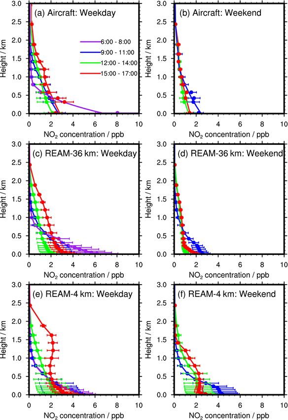
https://doi.org/10.5194/acp-21-11133-2021 Atmos. Chem. Phys., 21, 11133–11160, 202111144 J. Li et al.: Effects of resolution-dependent representation of NOx emissions Figure 8. Temporal evolutions of NO2 vertical profiles below 3 km on (a, c, e) weekdays and (b, d, f) weekends from the (a, b) P-3B aircraft and (c, d) 36 km and (e, f) 4 km REAM during the DISCOVER-AQ campaign. Horizontal bars denote the corresponding standard deviations. In (a, b), dots denote aircraft measurements, while lines below 1 km are based on quadratic polynomial fitting, as described in Sect. 2.6. The fitting values are mostly in reasonable agreement with the aircraft and surface measurements in the boundary layer. On weekends, no aircraft observations were made between 06:00 and 08:00 LT, and therefore no corresponding model profiles are shown. tochemical loss of NOx in the late afternoon. In fact, photo- and 7, observed and simulated concentrations of NO2 are chemical losses affect all the daytime NO2 vertical profiles, lower on weekends than on weekdays. Some of the varia- which can be easily identified by NO2 TVCD process diag- tions from weekend profiles are due to a lower number of ob- nostics discussed in Sect. 3.4 (Fig. 9). servations (47 spirals) on weekends. The overall agreement Figure 8b and d also show the observed and 36 km REAM- between the observed vertical profiles and 36 km model re- simulated vertical profiles on weekends. Similar to Figs. 5 sults is good on weekends (R 2 = 0.87). Between 15:00 and Atmos. Chem. Phys., 21, 11133–11160, 2021 https://doi.org/10.5194/acp-21-11133-2021
J. Li et al.: Effects of resolution-dependent representation of NOx emissions                                                      11145

Figure 9. Contributions of emission, chemistry, transport, and dry deposition to NOx TVCD diurnal variations over the 11 inland Pandora
sites (Table S1 and Fig. 1) on weekdays in July 2011 for the (a) 36 km and (b) 4 km REAM simulations. “Chem” refers to net NOx chemistry
production; “Emis” refers to NOx emissions; “Drydep” denotes NOx dry depositions; “Transport” includes advection, turbulent mixing,
lightning NOx production, and wet deposition. “Total (NOx )” is the hourly change in NOx TVCDs ((TVCD) = TVCDt+1 − TVCDt ). “Total
(NO2 )” is the hourly change in NO2 TVCDs, and “Total (NO)” is the hourly change in NO TVCDs.

17:00 LT, the model simulates a larger gradient than what the         3.4   Daytime variation in NO2 TVCDs
combination of aircraft and surface measurements indicates.
It may be related to the somewhat underestimated MLHs in              We compare satellite, P-3B aircraft, and model-simulated
the late afternoon in the model (Fig. 6).                             TVCDs with Pandora measurements, which provide contin-
   On weekdays, most simulated vertical profiles at the 4 km          uous daytime observations. The locations of Pandora sites
resolution (Fig. 8e) are similar to 36 km results in part be-         are shown in Table S1 and Fig. 1. Among the Pandora
cause the average NOx emissions over the six P-3B spiral              sites, four sites are located significantly above the ground
sites are about the same, 4 % lower in the 4 km than the              level: UMCP (∼ 20 m), UMBC (∼ 30 m), SERC (∼ 40 m),
36 km REAM simulations (Table S1). A clear exception is               and GSFC (∼ 30 m). The other sites are 1.5 m a.g.l. To prop-
the 4 km REAM-simulated vertical profile Between 15:00                erly compare Pandora to other measurements and model
and 17:00 LT when the model greatly overestimates bound-              simulations, we calculate the missing TVCDs between the
ary layer NOx mixing and concentrations. The main reason is           Pandora site heights and ground surface by multiplying the
that WRF-simulated vertical velocities (W ) in the late after-        Pandora TVCDs with model-simulated TVCD fractions of
noon are much larger in the 4 km simulation than the 36 km            the corresponding columns. The resulting correction is 2 %–
                                                                                         1
simulation (Fig. S9), which can explain the simulated fully           21 % ( 1−missing TVCD   percentage ) for the four sites significantly
mixed boundary layer between 15:00 and 17:00 LT. Since it             above the ground surface, but the effect on the averaged day-
is not designed to run at the 4 km resolution, and it is com-         time TVCD variation at all Pandora sites is small (Fig. S12).
monly assumed that convection can be resolved explicitly              In the following analysis, we use the updated Pandora TVCD
at high resolutions, the Kain–Fritsch (new Eta) convection            data.
scheme is not used in the nested 4 km WRF simulation (Ta-                The weekday diurnal variations in NO2 TVCDs from
ble S2); it may be related to the large vertical velocities in        satellites, Pandora, 4 and 36 km REAM, and the P-3B aircraft
the late afternoon, when thermal instability is the strongest.        are shown in Fig. 10a. We calculate aircraft-derived TVCDs
Appropriate convection parameterization is likely still nec-          by using Eq. (1):
essary for 4 km simulations (Zheng et al., 2016), which may                               P
                                                                                              caircraft (t) · ρREAM (t) · VREAM (t)
also help alleviate the underestimation of precipitation in the       TVCDaircraft (t) =                                            , (1)
nested 4 km WRF simulation as discussed in Sect. 3.1.                                                         AREAM
   The same rapid boundary layer mixing due to vertical               where t is time, caircraft (v/v) denotes aircraft NO2 con-
transport is present in the 4 km REAM-simulated weekend               centrations (mixing ratios) at each level at time t, ρREAM
vertical profile (Fig. 8f), although the mixing height is lower.      (molecules cm−3 ) is the density of air from 36 km REAM
Fewer spirals (47) and distinct transport effect due to dif-          at the corresponding level, VREAM (cm3 ) is the volume
ferent NO2 horizontal gradients between the 4 and 36 km               of the corresponding 36 km REAM grid cell, and AREAM
REAM simulations (discussed in detail in Sect. 3.6) may               (cm2 ) is the surface area (36 km × 36 km). In the calcula-
cause the overestimation of weekend profiles in the 4 km              tion, we only use NO2 concentrations below 3.63 km a.g.l.
REAM simulation.                                                      because few aircraft measurements were available above this

https://doi.org/10.5194/acp-21-11133-2021                                            Atmos. Chem. Phys., 21, 11133–11160, 2021
You can also read