An energy balance model for paleoclimate transitions - Climate of the Past
←
→
Page content transcription
If your browser does not render page correctly, please read the page content below
Clim. Past, 15, 493–520, 2019
https://doi.org/10.5194/cp-15-493-2019
© Author(s) 2019. This work is distributed under
the Creative Commons Attribution 4.0 License.

An energy balance model for paleoclimate transitions
Brady Dortmans, William F. Langford, and Allan R. Willms
Department of Mathematics and Statistics, University of Guelph, 50 Stone Road West, Guelph, ON, N1G 2W1, Canada

Correspondence: William F. Langford (wlangfor@uoguelph.ca)

Received: 8 May 2018 – Discussion started: 22 May 2018
Revised: 23 February 2019 – Accepted: 26 February 2019 – Published: 21 March 2019

Abstract. A new energy balance model (EBM) is presented           climate transitions in the past, with a focus on transitions that
and is used to study paleoclimate transitions. While most pre-    were abrupt. The understanding gained here will be applied
vious EBMs only dealt with the globally averaged climate,         in a subsequent paper to the important problem of determin-
this new EBM has three variants: Arctic, Antarctic and tropi-     ing whether anthropogenic climate change may lead to an
cal climates. The EBM incorporates the greenhouse warm-           abrupt transition in the future.
ing effects of both carbon dioxide and water vapour, and             We present a new two-layer energy balance model (EBM)
also includes ice–albedo feedback and evapotranspiration.         for the climate of the Earth. General knowledge of climate
The main conclusion to be inferred from this EBM is that          and of climate change has been advanced by many studies
the climate system may possess multiple equilibrium states,       employing simple EBMs (Budyko, 1968; Kaper and Engler,
both warm and frozen, which coexist mathematically. While         2013; McGehee and Lehman, 2012; North et al., 1981; Payne
the actual climate can exist in only one of these states at any   et al., 2015; Sagan and Mullen, 1972; Sellers, 1969; Stap
given time, the EBM suggests that climate can undergo tran-       et al., 2017). In general, these EBMs facilitate exploration
sitions between the states via mathematical saddle-node bi-       of the relationship between specific climate forcing mecha-
furcations. This paper proposes that such bifurcations have       nisms and the resulting climate changes. The EBM presented
actually occurred in Paleoclimate transitions. The EBM is         here includes a more accurate representation of the role of
applied to the study of the Pliocene paradox, the glacia-         greenhouse gases in climate change than has been the case
tion of Antarctica and the so-called warm, equable climate        for previous EBMs. The model is based on fundamental prin-
problem of both the mid-Cretaceous Period and the Eocene          ciples of atmospheric physics, such as the Beer–Lambert law,
Epoch. In all cases, the EBM is in qualitative agreement with     the Stefan–Boltzmann law, the Clausius–Clapeyron equation
the geological record.                                            and the ideal-gas equation. In particular, the modelling of wa-
                                                                  ter vapour acting as a greenhouse gas in the atmosphere, pre-
                                                                  sented in Sect. 2.3.3, is more physically accurate than in pre-
                                                                  vious EBMs and it shows that water vapour feedback is im-
1   Introduction                                                  portant in climate change. Also, ice–albedo feedback plays
                                                                  a central role in this EBM. The nonlinearity of this EBM
For approximately 75 % of the last 540 million years of the       leads to bistability (existence of multiple stable equilibrium
paleoclimate history of the Earth, the climate of both polar      states), to hysteresis (the climate state realized in the model
regions was mild and free of permanent ice-caps (Cronin,          depends on the past history) and to bifurcations (abrupt tran-
2010; Crowley, 2000; Hubert et al., 2000). Today, both the        sitions from one state to another). Forcing factors that are
North and South poles are ice-capped; however, there is over-     included explicitly in the model include insolation, CO2 con-
whelming evidence that these polar ice-caps are melting. The      centration, relative humidity, evapotranspiration, ocean heat
Arctic is warming faster than any other region on Earth. The      transport and atmospheric heat transport. Other factors that
formation of the present-day Arctic and Antarctic ice-caps        may affect climate change, such as geography, precipitation,
occurred abruptly, at widely separated times in the geolog-       vegetation and continental drift, are not included explicitly
ical history of the Earth. This paper explores some of the
underlying mechanisms and forcing factors that have caused

Published by Copernicus Publications on behalf of the European Geosciences Union.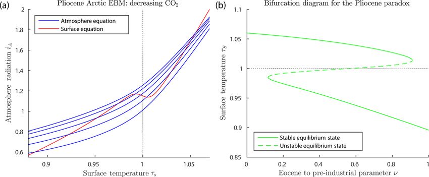
494                                                                      B. Dortmans et al.: EBM for paleoclimate transitions

in the EBM but are present only implicitly in so far as they       (2011) and Sloan and Barron (1990, 1992) observed that the
affect those included factors.                                     early Eocene (56–48 Ma) encompasses the warmest climates
   During the Pliocene Epoch, 2.6–5.3 Ma, the climate of the       of the past 65 million years, yet climate modelling studies
Arctic region of Earth changed abruptly from ice-free to ice-      had difficulty explaining such warm and equable tempera-
capped. The major climate forcing factors (solar constant,         tures. Therefore, this situation was called the early Eocene
orbital parameters, CO2 concentration and locations of the         warm, equable climate problem. The EBM of the present pa-
continents) were all very similar to today (Fedorov et al.,        per suggests that the mathematical mechanism of bistability
2006, 2010; Haywood et al., 2009; Lawrence et al., 2009;           provides plausible answers to both the mid-Cretaceous and
De Schepper et al., 2015). Therefore, it is difficult to explain   the early Eocene equable climate problems. In fact, from the
why the early Pliocene climate was so different from that of       perspective of this simple model, these two are mathemati-
today. That problem has been called the Pliocene paradox           cally the same problem. Therefore, we call them collectively
(Cronin, 2010; Fedorov et al., 2006, 2010). Currently, there       the warm, equable Paleoclimate problem. Recent progress
is great interest in mid-Pliocene climate as a natural ana-        in paleoclimate science has succeeded in narrowing the gap
logue of the future warmer climate expected for Earth, due         between proxy and general circulation model (GCM) esti-
to anthropogenic forcing. In recent years, significant progress    mates for the Cretaceous climate (Donnnadieu et al., 2006;
has been achieved in understanding Pliocene climate, e.g. by       Ladant and Donnadieu, 2016; O’Brien et al., 2017) and for
Haywood et al. (2009); Salzmann et al. (2009); Ballantyne          the Eocene climate (Baatsen et al., 2018; Hutchinson et al.,
et al. (2010); Steph et al. (2010); von der Heydt and Dijk-        2018; Lunt et al., 2016, 2017).
stra (2011); Zhang and Yan (2012); Zhang et al. (2013); Sun           The principal contribution of this paper is a simple cli-
et al. (2013); De Schepper et al. (2013); Tan et al. (2017);       mate EBM, based on fundamental physical laws, that ex-
Chandan and Peltier (2017, 2018) and Fletcher et al. (2018);       hibits bistability, hysteresis and bifurcations. We propose that
see also references therein. This paper proposes that bista-       these three phenomena have occurred in the paleoclimate
bility and bifurcation may have played a fundamental role in       record of the Earth and they help to explain certain paleocli-
determining the Pliocene climate.                                  mate transitions and puzzles as outlined above. A key prop-
   The waning of the warm ice-free paleoclimate at the South       erty of this EBM is that its underlying physical principles are
Pole, leading eventually to abrupt glaciation of Antarctica at     highly nonlinear. As is well known, nonlinear equations can
the Eocene–Oligocene transition (EOT) about 34 Ma, is be-          have multiple solutions, unlike linear equations, which can
lieved to have been caused primarily by two major geologi-         have only one unique solution (if well-posed). In our EBM,
cal changes (although other factors played a role). One is the     the same set of equations can have two or more coexisting
movement of the continent of Antarctica from the Southern          stable solutions (bistability); for example, an ice-capped so-
Pacific Ocean to its present position over the South Pole, fol-    lution (like today’s climate) and an ice-free solution (like the
lowed by the development of the Antarctic Circumpolar Cur-         Cretaceous climate), even with the same values of the forc-
rent (ACC), thus drastically reducing ocean heat transport to      ing parameters. The determination of which solution is ac-
the South Pole (Cronin, 2010; Scher et al., 2015). The second      tually realized by the planet at a given time is dependent
is the gradual draw down in CO2 concentration worldwide            on past history (hysteresis). Changes in forcing parameters
(DeConto et al., 2008; Goldner et al., 2014; Pagani et al.,        may drive the system abruptly from one stable state to an-
2011). The EBM of this paper includes both CO2 concen-             other, at so-called “tipping points”. In this paper, these tip-
tration and ocean heat transport as explicit forcing factors.      ping points are investigated mathematically, and are shown
The results of this paper suggest that the abrupt glaciation       to be bifurcation points, which are investigated using math-
of Antarctica at the EOT was the result of a bifurcation that      ematical bifurcation theory. Bifurcation theory tells us that
occurred as both of these factors changed incrementally; and       the existence of bifurcation points is preserved (but the nu-
furthermore that both are required to explain the abrupt onset     merical values may change) under small deformations of the
of Antarctic glaciation.                                           model equations. Thus, even though this conceptual model
   In the mid-Cretaceous Period (100 Ma) the climate of the        may not give us precise quantitative information about cli-
entire Earth was much more equable than it is today. This          mate changes, qualitatively there is good reason to believe
means that, compared to today, the pole-to-Equator tempera-        that the existence of the bifurcation points in the model will
ture gradient was much smaller and also the summer/winter          be preserved in similar more refined models and in the real
variation in temperature at mid- to high-latitudes was much        world.
less (Barron, 1983). The differences in forcing factors be-           Previous climate models exhibiting multiple equilibrium
tween the Cretaceous Period and modern times appeared to           states have indicated that bifurcations may cause abrupt cli-
be insufficient to explain this difference in the climates. Eric   mate transitions (Budyko, 1968; Sellers, 1969; North et al.,
Barron called this the warm, equable Cretaceous climate            1981; Paillard, 1998; Alley et al., 2003; Rial et al., 2004;
problem and he explored this problem in a series of pioneer-       Lindsay and Zhang, 2005; Ferreira et al., 2010; Thorndike,
ing papers (Barron, 1983; Barron et al., 1981, 1995; Sloan         2012; Payne et al., 2015; Stap et al., 2017). None of these
and Barron, 1992). In a similar vein, Huber and Caballero          authors employ the recently developed mathematical the-

Clim. Past, 15, 493–520, 2019                                                                  www.clim-past.net/15/493/2019/
B. Dortmans et al.: EBM for paleoclimate transitions                                                                         495

ory of bifurcations to the extent used in this paper. Abrupt         The energy balance model presented here is conceptual
transitions in Quaternary glaciations have been studied by        and qualitative. It contains many simplifying assumptions
Ganopolski and Rahmstorf (2001); Paillard (2001a, b); Calov       and is not intended to give a detailed description of the cli-
and Ganopolsky (2005) and Robinson et al. (2012). These           mate of the Earth with quantitative precision. It complements
glacial cycles are strongly influenced by orbital forcings,       but does not replace more detailed GCMs. Geographically,
which are not within the scope of this paper. Scientists have     this model is as simple as possible. It follows in a long tradi-
long considered that abrupt transitions (or bifurcations) in      tion of slab models of the atmosphere. Previous slab models
the Atlantic Meridional Overturning Circulation (AMOC)            represented the atmosphere of the Earth as a globally aver-
were possible, and that this could contribute to abrupt cli-      aged uniform slab at a single temperature T . The temperature
mate change (Stommel, 1961; Rahmstorf, 1995; Ganopol-             T is determined in those models by a global energy balance
ski and Rahmstorf, 2001; Lenton et al., 2012). This type of       equation of the form energy in = energy out. Such models are
change in the AMOC is sometimes called a Stommel bifurca-         unable to differentiate between different climates at different
tion. However, that phenomenon is also outside the scope of       latitudes; for example, if the polar climate is changing more
the EBM of this paper, which does not include ocean geogra-       rapidly than the tropical climate. In this new model, the forc-
phy or meridional dependence. (An extension of this EBM,          ing parameters of the slab atmosphere are chosen to represent
to a partial differential equation (PDE) spherical shell model,   each one of three particular latitudes: Arctic, Antarctic or
is planned.)                                                      tropics. Each of these regions is represented by its own slab
   With regard to the EOT, a variety of indicators, includ-       model, with its own forcing parameters and its own surface
ing the analysis of fossil plant stomata (Steinthorsdottir et     temperature TS . In addition, each region has its own variable
al., 2016), imply that decreasing atmospheric pCO2 in the         IA representing the intensity of the radiation re-emitted by
Eocene preceded the large shift in oxygen isotope records         the atmosphere. The two independent variables IA and TS are
that characterize the EOT. It was hypothesized in Steinthors-     determined in each model by two energy balance equations,
dottir et al. (2016) that at the EOT, a certain threshold of      expressing energy balance in the atmosphere and energy bal-
pCO2 was crossed, resulting in an abrupt change of climate        ance at the surface, respectively. In this way, the different
mode. Possible mechanisms for the threshold that they hy-         climate responses of these three regions to their respective
pothesized are studied in Sect. 3.2.                              forcings can be explored.
   Even for changes as recent as the mid-Holocene, there             The role played by greenhouse gases in climate change is
is a debate, for example, over whether the abrupt deserti-        a particular focus of this model. Greenhouse gases trap heat
fication of the Sahara is due to a bifurcation, as suggested      emitted by the surface and are major contributors to global
in Claussen et al. (1999) using an Earth model of interme-        warming. The very different roles of the two principal green-
diate complexity (EMIC), or is a transient response of the        house gases in the atmosphere, carbon dioxide and water
AMOC to a sudden termination of freshwater discharge to           vapour, are analyzed here in Sects. 2.3.2 and 2.3.3, respec-
the North Atlantic, as proposed in Liu et al. (2009), using a     tively. The greenhouse warming effect of CO2 increases with
coupled atmosphere–ocean GCM (AOGCM). Similarly, for              the density of the atmosphere but is independent of temper-
the glaciation of Greenland at the Pliocene–Pleistocene tran-     ature, while the greenhouse warming of H2 O increases with
sition, recent work in Tan et al. (2018), using a coupled         temperature but is independent of the density (or partial pres-
GCM–ice-sheet model, shows good agreement with proxy              sure) of the other gases present. The greenhouse warming of
records without the need for bifurcations. The model of this      methane (CH4 ) acts in a similar fashion to that of CO2 ; there-
paper does not adapt to these two situations, which are lo-       fore, CH4 can be incorporated into the CO2 concentration. As
calized and away from the poles where the axis of symmetry        an increase in CO2 concentration causes climate warming,
restricts the dynamics and facilitates the analysis presented     this warming causes an increase in evaporation of H2 O into
here.                                                             the atmosphere, which further increases the climate warming
   Further investigation of climate changes, using a range of     beyond that due to CO2 alone (this is true both in the model
climate models from EBM and EMIC to GCM and AOGCM,                and in the real atmosphere). This effect is known as water
is warranted to clarify the underlying mechanisms of abrupt       vapour feedback. The energy balance model presented here
climate change. Very sophisticated GCMs, which include            is the first EBM to incorporate these important roles of the
many 3-D processes, are only able to run a few climate tra-       greenhouse gases in such detail.
jectories; while EBMs and EMICs may explore more pos-                The paper concludes with two appendices. In Appendix A,
sibilities and investigate climate transitions (tipping points)   model parameters that are difficult or impossible to deter-
with major simplifications and with less effort. More rig-        mine for paleoclimates are calibrated using the abundant
orous mathematical analysis is possible on small models,          satellite and surface data available for today’s climate. In
which may then suggest lines of inquiry on large models. The      addition, justification is given for parameter values chosen
Earth climate system is extremely complex. For best results,      for the model. In Appendix B the paleoclimate model of this
a hierarchy of climate models is necessary.                       paper is adapted to modern-day conditions and its equilib-
                                                                  rium climate sensitivity (ECS) is determined. Here, ECS is

www.clim-past.net/15/493/2019/                                                                  Clim. Past, 15, 493–520, 2019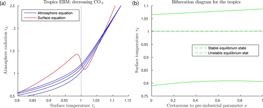
496                                                                         B. Dortmans et al.: EBM for paleoclimate transitions

Table 1. Summary of variables and parameters used in the model. Many of these parameters have standard textbook values (e.g.
TR , σ, Lv , RW ). The standard lapse rate 0 is from ICAO (1993). Other parameters such as kC and kW are derived in Appendix A.

                                                   Variables and parameters used
      Variables                                        Symbol            Values
      Mean temperature of the surface                  TS                −50 to +20 ◦ C
      Infrared radiation from the surface              IS                141 to 419 W m−2
      Mean temperature of the atmosphere               TA                −70 to 0 ◦ C
      Energy emitted by the atmosphere                 IA                87 to 219 W m−2
      Parameters and constants                         Symbol            Values
      Temperature of freezing point for water          TR                273.15 K
      Stefan–Boltzmann constant                        σ                 5.670 × 10⁻⁸ W m−2 K−4
      Emissivity of dry air                                             0.9
      Fraction of IA reaching surface                  β                 0.63
      Incident solar radiation                         Q                 173.2 W m−2 (poles), 418.8 W m−2 (Equator)
      Fraction of solar radiation reflected from       ξR                0.2235
      atmosphere
      Fraction of solar radiation directly absorbed    ξA                0.2324
      by atmosphere
      Warm surface albedo                              αW                0.08 to 0.15
      Cold surface albedo                              αC                0.7
      Albedo transition rate (in tanh function)        ω = /TR          0.01
      Solar radiation striking surface                 FS                (1 − ξR − ξA )Q
      Ocean heat transport                             FO                −55 to 100 W m−2
      Atmospheric heat transport                       FA                −25 to 45 W m−2
      Vertical heat transport (conduction              FC                0 to 150 W m−2 , function of TS
      + evapotranspiration)
      Vertical heat transport coefficients             a1 , a2           2.650 and 6.590 × 10⁻² , respectively
      Molar concentration of CO2 in ppm                µ                 270 to 1600 ppm
      Relative humidity of H2 O                        δ                 0.5 to 0.85
      Absorptivity for CO2                             ηC                0 to 1, function of µ
      Absorptivity for H2 O                            ηW                0 to 1, function of δ and TS
      Absorptivity for clouds                          ηCl               0.3729
      Total atmosphere absorptivity                    η                 1 − (1 − ηW )(1 − ηC )(1 − ηCl )
      Grey gas absorption coefficient for CO2          kC                0.07424 m2 kg−1
      Grey gas absorption coefficient for H2 O         kW                0.05905 m2 kg−1
      Standard and normalized atmosphere lapse rates   0, γ = 0/TR       6.49 × 10⁻³ K m−1 and 2.38 × 10⁻⁵ m−1 , respectively
      Tropopause height                                Z                 9 km (poles), 17 km (Equator), 14 km (global)
      Latent heat of vaporization of water             Lv                2.2558 × 10⁶ m2 s−2
      Ideal-gas constant specific to water vapour      RW                461.5 m2 s−2 K−1
      Saturated partial pressure of water at TR        PWsat (T )        611.2 Pa
                                                               R
      Atmospheric standard pressure at surface         PA                101.3 × 10³ Pa
      Gravitational acceleration                       g                 9.81 m s−2
      Parameter for ηC                                 GC                (1.52 × 10⁻⁶ )kC PA /g = 1.166 × 10⁻³
      First parameter for ηW                           GW1               Lv /(RW TR ) = 17.89
      Second parameter for ηW                          GW2               kW PW sat (T )/(γ R T ) = 12.05
                                                                                     R      W R

the change in global mean temperature produced by a dou-             2    The energy balance climate model
bling of CO2 in the model, starting from the pre-industrial
value of 270 ppm. For this EBM, the ECS is determined to             In this EBM, the atmosphere and surface are each assumed
be 1T = 3.3 ◦ C, which is at the high end of the range ac-           to be in energy balance. Short-wave radiant energy from the
cepted by the IPCC (IPCC, 2013).                                     sun is partly reflected by the atmosphere back into space, a
                                                                     small portion is absorbed directly by the atmosphere and the
                                                                     remainder passes through to the surface. The surface reflects

Clim. Past, 15, 493–520, 2019                                                                      www.clim-past.net/15/493/2019/
B. Dortmans et al.: EBM for paleoclimate transitions 497
FO and FA represent ocean and atmosphere heat transport,
respectively, and are specified as constants for each region
of interest. Heat transport by conduction/convection from
the surface to the atmosphere is denoted FC . This quantity
will be largely dependent on surface temperature, TS . As de-
scribed in Appendix A we have modelled it as a hyperbola
that is mostly flat for temperatures below freezing, and grows
Figure 1. A visualization of the energy balance model. Symbols are roughly linearly for temperatures above freezing so that
defined in Table 1 and Sect. 2.1. q
FC = A1 (TS − TR ) + A21 (TS − TR )2 + A22 , (3)
where A1 and A2 are constants. Since the model is concerned
some of this short-wave energy (which is assumed to escape
with temperatures around the freezing point of water, we set
to space) and absorbs the rest, re-emitting long-wave radiant
this as a reference temperature, TR = 273.15 K.
energy of intensity IS upward into the atmosphere. The at-
The annually averaged intensity of solar radiation strik-
mosphere is modelled as a slab, with greenhouse gases, that
ing a surface parallel to the Earth’s surface but at the top
absorbs a fraction η of the radiant energy IS from the surface.
of the atmosphere is Q. The value of Q at either Pole is
The atmosphere re-emits radiant energy of total intensity IA .
Q = 173.2 Wm−2 and at the Equator is 418.8 Wm−2 (McGe-
Of this radiation IA , a fraction β is directed downward to the
hee and Lehman, 2012; Kaper and Engler, 2013). A fraction
surface, and the remaining fraction (1 − β) goes upward and
ξR of this short-wave radiation is reflected by the atmosphere
escapes to space.
back into space and a further fraction ξA is directly absorbed
This model is based on the uniform slab EBM used in
by the atmosphere; the remainder penetrates to the surface.
Payne et al. (2015), modified as shown in Fig. 1. In our case,
See Appendix A1 for the derivation of values for ξR and ξA .
the “slab” is a uniform column of air of unit cross section,
The solar radiation striking the surface of the Earth is
extending vertically above the surface to the tropopause, and
located either at a pole or at the Equator. The symbols in
Fig. 1 are defined in Table 1. FS = (1 − ξR − ξA )Q. (4)
This section presents the mathematical derivation of the
EBM. Readers interested only in the climate applications of The surface albedo is the fraction, α, of this solar radiation
the model may skip this section and go directly to Sect. 3. A that reflects off the surface back into space. Thus the solar
preliminary version of this EBM was presented in a confer- forcing absorbed by the surface is (1 − α)FS , and the solar
ence proceedings paper (Dortmans et al., 2018). The present radiation reflected back to space is αFS . Typical values of
model incorporates several important improvements over the surface albedo α are 0.6–0.9 for snow, 0.4–0.7 for ice, 0.2
that model. The differences between that model and the one for crop land and 0.1 or less for open ocean. In this paper we
presented here are indicated where appropriate in the text. introduce a smoothly varying albedo given by the hyperbolic
Furthermore, the previous paper (Dortmans et al., 2018) con- tangent function:
sidered only the application of the model to the Arctic cli-
mate and the Pliocene paradox; it did not study Antarctic 1 TS − TR
α= [αW + αC ] + [αW − αC ] tanh , (5)
or tropical climate or the Cretaceous warm, equable climate 2
problem, as does the present paper. where αC and αW are the albedo values for cold and warm
temperatures, respectively, and the parameter determines
2.1 Energy balance the steepness of the transition between αC and αW . See Ap-
pendix A2 for a full explanation of Eq. (5).
The model consists of two energy balance equations, one for
The emission of long-wave radiation, I , from a body is
the atmosphere and one for the surface. In Fig. 1, the so-
governed by the Stefan–Boltzmann law, I = σ T 4 , where
called forcings are shown as arrows, pointing in the direction
is the emissivity, σ is the Stefan–Boltzmann constant, and T
of energy transfer. From Fig. 1, the energy balance equations
is temperature. The surface of the Earth acts as a black-body
for the atmosphere and surface are given, respectively, by
radiator; so for the radiation emitted from the surface = 1,
thus
0 = FA + FC + ξA Q + ηIS − IA , and (1) IS = σ TS4 . (6)
0 = FO − FC + (1 − α)FS − IS + βIA . (2) Previous authors have postulated an idealized uniform at-
mospheric temperature TA for the slab model, so that the in-
Symbols and parameter values for the model are defined
tensity of radiation emitted by the atmosphere, IA , is
in Table 1. Appendix A4 provides derivations and justifica-
tion for the values of the empirical parameters. The forcings IA = σ TA4 . (7)
www.clim-past.net/15/493/2019/ Clim. Past, 15, 493–520, 2019498 B. Dortmans et al.: EBM for paleoclimate transitions
The emissivity is = 0.9 since the atmosphere is an imper- 273.15 K, and therefore the nondimensional temperature τ
fect black-body radiator. A uniform temperature for the at- lies in an interval around τ = 1. In this paper, we assume
mosphere does not exist in the real world, where TA varies 0.8 ≤ τ ≤ 1.2, which corresponds approximately to a range
strongly with height, unlike TS , which has a single value. in more familiar degrees Celsius of −54 ◦ C ≤ T ≤ +54 ◦ C.
Previous two-layer EBMs have used (TS , TA ) as the two inde- Another reason for the upper limit on temperature is that the
pendent variables in the two energy balance Eqs. (1) and (2). Clausius–Clapeyron law used in Sect. 2.3.3 fails to apply at
Here instead, we use (TS , IA ) as the two independent vari- temperatures above the boiling point of water.
ables, and then we formally let TA be defined by Eq. (7). The
fraction of IA that reaches the surface is β = 0.63; see Ap-
2.2 Optical depth and the Beer–Lambert law
pendix A6.
The parameter η represents the fraction of the infrared The goal of this section is to define the absorptivity param-
radiation IS from the surface that is absorbed by the atmo- eter η in the EBM Eq. (9) (or Eq. 1) in such a way that the
sphere and is called absorptivity. The major constituents of atmosphere in the uniform slab model will absorb the same
the atmosphere are nitrogen and oxygen and these gases do fraction η of the long-wave radiation IS from the surface
not absorb any infrared radiation. The gases that do con- as does the real nonuniform atmosphere of the Earth. This
tribute to the absorptivity η are called greenhouse gases. absorption is due primarily to water vapour, carbon dioxide
Chief among these are carbon dioxide and water vapour. The and clouds. Previous energy balance models have assigned a
contribution of these two greenhouse gases to η are analyzed constant value to η, often determined by climate data. In the
in Sects. 2.3.2 and 2.3.3, respectively. Although both con- present EBM, η is not constant but is a function of other more
tribute to warming of the climate, the underlying physical fundamental physical quantities, such as µ, δ, kC , kW and T .
mechanisms of the two are very different. In general, the This function is determined by classical physical laws. In
contribution to η from water vapour is a function of temper- this way, the present EBM adjusts automatically to changes
ature. Another major contributor to absorption is the liquid in these physical quantities, and represents a major advance
and solid water in clouds. We model this portion of the ab- over previous EBMs.
sorption as constant, since we do not include any data on The Beer–Lambert law states that when a beam of radi-
cloud cover variation. However, we experimented with mak- ation (or light) enters a sample of absorbing material, the
ing this portion vary with surface temperature, and the results absorption of radiation at any point z is proportional to the
were not qualitatively different than those presented here. intensity of the radiation I (z) and also to the concentration
or density of the absorber ρ(z). This bilinearity fails to hold
Nondimensional temperatures at very high intensity of radiation or high density of ab-
sorber, neither of which is the case in the Earth’s atmosphere.
We rescale temperature by the reference temperature TR = Whether this law is applied to the uniform slab model or to
273.15 K and define new nondimensional temperatures and the nonuniform real atmosphere, it yields the same differen-
new parameters tial equation
TS IA Q FO FA
τS = , iA = 4
, q= 4
, fO = 4
, fA = , dI
TR σ TR σ TR σ TR σ TR4 = −kρ(z)I (z), (13)
dz
FC A1 A2
fC = , a1 = , a2 = , ω= . (8)
4
σ TR 3
σ TR σ TR4 TR where k (m2 kg−1 ) is the absorption coefficient of the ma-
terial, ρ (kg m−3 ) is the density of the absorbing substance
After normalization, the freezing temperature of water is such as CO2 and z (m) is distance along the path. The differ-
represented by τ = 1 and the atmosphere and surface energy ential Eq. (13) may be integrated from z = 0 (the surface) to
balance Eqs. (1)–(6) simplify to z = Z (the tropopause) to give
iA = fA + fC (τS ) + ξA q + η(τS )τS4 , (9)
ZZ
1h i IT RZ
iA = fC (τS ) − fO − (1 − α(τS ))(1 − ξR − ξA )q + τS4 , (10) = e− 0 kρ(z) dz ≡ e−λ , where λ ≡ kρ(z) dz. (14)
β IS
0
where, from Appendix A,
q Here IT ≡ I (Z) is the intensity of radiation escaping to space
fC (τS ) = a1 (τS − 1) + a12 (τS − 1)2 + a22 , (11) at the tropopause z = Z, and λ is the so-called optical depth
1
τS − 1
of the material. Note that λ is dimensionless. The absorptiv-
α(τS ) = [αW + αC ] + [αW − αC ] tanh . (12) ity parameter η in Eqs. (1) and (9) represents the fraction of
2 ω
the outgoing radiation IS from the surface that is absorbed
The range of surface temperatures TS observed on Earth is by the atmosphere (not to be confused with the absorption
restricted to an interval around the freezing point of water, coefficient k). It follows from the Beer–Lambert law that η
Clim. Past, 15, 493–520, 2019 www.clim-past.net/15/493/2019/B. Dortmans et al.: EBM for paleoclimate transitions 499
is completely determined by the corresponding optical depth dry air, and written as µ. There is convincing evidence that µ
parameter λ; that is has varied greatly in the geological history of the Earth, and
has decreased slowly over the past 100 million years; how-
IS − IT ever, today µ is increasing due to human activity. The value
η= = 1 − e−λ . (15)
IS before the industrial revolution was µ = 270 ppm, but today
For a mixture of n attenuating materials, with densities ρi , µ is slightly above 400 ppm.
absorption coefficients ki and corresponding optical depths Although traditionally µ is measured as a ratio of molar
λi , the Beer–Lambert law extends to concentrations, in practice both the density ρ and the ab-
sorption coefficient k are expressed in mass units of kilo-
IT n
RZ n grams. Therefore, before proceeding, µ must be converted
= e−6i=1 0 ki ρi (z) dz ≡ e−6i=1 λi , (16)
IS from a molar ratio to a ratio of masses in units of kilograms.
The mass of one mole of CO2 is approximately mmC =
so that 44×10−3 kg mol−1 . The dry atmosphere is a mixture of 78 %
n
n
Y n
Y nitrogen, 21 % oxygen and 0.9 % argon, with molar masses
η = 1 − e−6i=1 λi = 1 − e−λi = 1 − (1 − ηi ), (17) of 28, 32 and 40 g mol−1 , respectively. Neglecting other trace
i=1 i=1 gases in the atmosphere, a weighted average gives the molar
mass of the dry atmosphere as mmA = 29 × 10−3 kg mol−1 .
where ηi = 1 − e−λi . Equation (17) is the key to solving the Therefore, the CO2 concentration µ measured in molar ppm
problem posed in the first sentence of this subsection. For the is converted to mass concentration in kg ppm by multiplica-
ith absorbing material in the slab model, we set its optical tion by the ratio mmC /mmA ≈ 1.52. If ρA (z) is the density
depth λi to be equal to the value of the optical depth that of the atmosphere at altitude z in kg m−3 , then the mass den-
this gas has in the Earth’s atmosphere as given by Eq. (14), sity of CO2 at the same altitude, with molar concentration
and then combine them using Eq. (16). This calculation is µ ppm, is
presented for the case of CO2 in Sect. 2.3.2 and for water
vapour in Sect. (2.3.3). For the third absorbing material in µ
ρC (z) = 1.52 ρA (z) kg m−3 . (18)
our model, clouds, we assume a constant value ηCl . 106
It is known that CO2 disperses rapidly throughout the Earth’s
2.3 Greenhouse gases atmosphere, so that its concentration µ may be assumed in-
The two principal greenhouse gases are carbon dioxide dependent of location and altitude (IPCC, 2013). As the den-
(CO2 ) and water vapour (H2 O). Because they act in differ- sity of the atmosphere decreases with altitude, the density of
ent ways, we determine the absorptivities ηC and ηW , and CO2 decreases at exactly the same rate, according to Eq. (18).
optical depths λC and λW of CO2 and H2 O separately, and Substituting Eq. (18) into Eq. (14) determines the optical
then combine their effects, along with the absorption due depth λC of CO2
to clouds, ηCl , using the Beer–Lambert law for mixtures,
ZZ
Eq. (17). Methane acts similarly to CO2 and can be included µ
in the optical depth for CO2 . Other greenhouse gases have λC = 1.52 kC ρA (z) dz. (19)
106
only minor influence and are ignored in this paper. 0
Now consider a vertical column of air, of unit cross sec-
2.3.1 The grey gas approximation tion, from surface to tropopause. The integral in Eq. (19)
Although it is well-known that gases like CO2 and H2 O ab- is precisely the total mass of this column. The atmospheric
sorb infrared radiation IS only at specific wavelengths (spec- pressure at the surfaceRis PA , and this is the total weight of
Z
tral lines), in this paper the grey gas approximation is used; the column. Therefore 0 ρ(A) dz = PA /g, where g is accel-
that is, the absorption coefficient kC or kW is given as a single eration due to gravity. Therefore, the optical depth λC of CO2
number averaged over the infrared spectrum (Pierrehumbert, in the actual atmosphere in Eq. (19) is
2010). The thesis by Dortmans (2017) presents a survey of PA
values in the literature for the absorption coefficients kC and λC = µGC , where GC ≡ 1.52 × 10⁻⁶ kC . (20)
g
kW of CO2 and H2 O, respectively, in the grey gas approxi-
mation. The values used in this paper are given in Table 1; With λC so determined, it follows from Eq. (15) that
and are derived as described in Appendix A5.
ηC = 1 − e−λC = 1 − exp(−µGC ). (21)
2.3.2 Carbon dioxide
As listed in Table 1 and derived in Appendix A5, the cali-
The concentration of CO2 in the atmosphere is usually ex- brated value for kC is 0.07424, and therefore the value for the
pressed as a ratio, in molar parts per million (ppm) of CO2 to greenhouse gas parameter for CO2 is GC = 1.166 × 10⁻³ .
www.clim-past.net/15/493/2019/ Clim. Past, 15, 493–520, 2019500 B. Dortmans et al.: EBM for paleoclimate transitions
Figure 2. Dry atmosphere EBM Eqs. (22)–(23) (with FA = 65 Wm−2 , FO = 50 Wm−2 , Q = 173.2 Wm−2 , αW = 0.08 and Z = 9 km).
(a) CO2 values µ = 400, 800, 1200, 1600, 2000; from bottom to top blue curves. A unique cold equilibrium exists for µ = 400 (bottom blue
curve), multiple equilibria exist for µ = 800, 1200 and 1600, a unique warm equilibrium exists for µ = 2000 (top blue curve). (b) Bifurcation
diagram for the same parameters as in (a) showing the result of solving the EBM for τS as a function of the forcing parameter µ, holding
all other forcing parameters constant. Two saddle-node (or fold) bifurcations occur at approximately µ = 681 and µ = 1881. Three distinct
solutions exist between these two values of µ. As µ decreases from right to left in this figure, if the surface temperature starts in the warm
state (τS > 1), then it abruptly “falls” from the warm state to the frozen state when the left bifurcation point is reached. Similarly, starting on
the frozen state (τS < 1), if µ increases sufficiently, then the state will jump upward to the warm branch when the right bifurcation point is
reached. Both of these transitions are irreversible (one way).
The dry atmosphere EBM is obtained by assuming there 2.3.3 Water vapour and the Clausius–Clapeyron
is no water vapour and no clouds in the atmosphere. Hence equation
η = ηC and δ = 0. We assume also that ξR = ξA = 0. Making
these substitutions in the EBM Eqs. (9)–(10) yields In this section, we determine the absorptivity of water vapour
as a function of temperature, ηW (τS ), using fundamental
physical laws including the Clausius–Clapeyron equation,
the ideal-gas law and the Beer–Lambert law (Pierrehum-
iA = fA + fC (τS ) + [1 − exp(−µGC )] · τS4 , (22)
bert, 2010). We also assume the idealized lapse rate of
1
the International Standard Atmosphere (ISA) as defined by
iA = fC (τS ) − fO − [1 − α(τS )]q + τS4 . (23)
β ICAO (ICAO, 1993). Unlike CO2 , the concentration of wa-
ter vapour (H2 O) in the atmosphere varies widely with lo-
cation and altitude. This is because the partial pressure of
Due to the nonlinearity of the ice–albedo function in 5, there H2 O varies strongly with the local temperature. In fact, it
can be in fact up to three points of intersection as shown in is bounded by a maximum saturated value, which itself is a
Fig. 2a. If the CO2 level µ decreases sufficiently, the warm nonlinear function of temperature, PW sat (T ). The actual partial
state (τS > 1) disappears, while as CO2 increases, the frozen pressure of water vapour is then a fraction, δ, of this saturated
state (τS < 1) may disappear. The CO2 level µ is quite ele- value,
vated in Fig. 2, but the effects of water vapour as a green-
house gas and of clouds have been ignored. sat
PW (T ) = δ PW (T ), 0 ≤ δ ≤ 1, (24)
Figure 2b introduces a bifurcation diagram (Kuznetsov,
2004), in which the two EBM Eqs. (22)–(23) have been where δ is called relative humidity. While PW sat (T ) varies
solved for the surface temperature τS , which is then plot- greatly with T in the atmosphere, the relative humidity δ
ted as a function of the parameter µ. Figure 2b shows the is comparatively constant. If the actual PW (T ) exceeds the
three distinct solutions τS of the EBM: a warm solution saturated value PW sat (T ) (i.e. δ > 1), the excess water vapour
(τS > 1), a frozen solution (τS < 1), and a third solution condenses out of the atmosphere and falls as rain or snow.
that crosses through τS = 1 and connects the other two so- The saturated partial pressure at temperature T is deter-
lutions in saddle-node bifurcations (Kuznetsov, 2004). Sta- mined by the Clausius–Clapeyron equation (Pierrehumbert,
bility analysis (Dortmans, 2017) shows that the warm and 2010),
frozen solutions are stable (in a dynamical systems sense),
while the third solution (denoted by a dashed line) is unsta- sat sat Lv 1 1
ble. PW (T ) = PW (TR ) exp − , (25)
RW TR T
Clim. Past, 15, 493–520, 2019 www.clim-past.net/15/493/2019/B. Dortmans et al.: EBM for paleoclimate transitions 501
where TR is the reference temperature, here chosen to be the z to τ . The result is
freezing point of water (273.15 K); Lv is the latent heat of
vaporization of water and RW is the ideal-gas constant for ZZ ZτS
kW
water, see Table 1. The actual partial pressure of water vapour λW = kW ρW (τ (z)) dz = ρW (τ ) dτ. (31)
γ
at relative humidity δ and temperature T is then given by 0 τS −γ Z
combining Eqs. (24) and (25).
We may use the ideal-gas law in the form PW = ρW RW T Now substitute Eq. (27) into the integral Eq. (31) and sim-
to convert the partial pressure PW of water vapour at temper- plify to
ature T to mass density ρW of water vapour at that tempera-
ZτS
ture. Substituting into Eqs. (24) and (25) gives 1 τ −1
λW (τS ) = δ GW2 exp GW1 dτ, (32)
sat (T ) τ τ
PW R Lv 1 1 τS −γ Z
ρW (T ) = δ exp − . (26)
RW T RW TR T
where the greenhouse gas parameters GW1 and GW2 for wa-
Transforming to the dimensionless temperature τ = T /TR as ter vapour are defined as
in Sect. 2.1, this becomes
sat (T )
kW P W
Lv R
sat
PW (TR ) 1
Lv
τ −1
GW1 ≡ and GW2 ≡ . (33)
ρW (τ ) = δ exp . (27) RW TR RW TR γ
RW TR τ RW TR τ
Finally, using the Beer–Lambert law, the absorptivity ηW of
The Beer–Lambert law in Sect. 2.2 implies that the absorp- water vapour in Eq. (28) is determined by its optical depth,
tivity of a greenhouse gas ηi is completely determined by its and is now a function of the surface temperature,
optical depth λi . For water vapour, from Eqs. (15) and (14),
ηW (τS ) = 1 − exp [−λW (τS )]
ZZ
−λW
ZτS
ηW = 1 − e where λW ≡ kW ρW (z) dz. (28) 1 τ −1
= 1 − exp −δ GW2 exp GW1 dτ . (34)
τ τ
0 τS −γ Z
Here kW is the absorption coefficient of water vapour; see The definite integral in this expression is easily evaluated nu-
Appendix A5. In order to evaluate the integral in Eq. (28), we merically in the process of solving the atmosphere and sur-
need to know how ρW varies with height z. We have shown face EBM equations. As given in Table 1 and derived in Ap-
that ρW is a function of temperature, given by Eqs. (26) pendix A5, the calibrated value of kW is 0.05905 m2 kg−1
or (27). Therefore, we need an expression for the variation in and the greenhouse gas parameters for H2 O are
temperature T with height z. Under normal conditions, the
temperature T decreases with height in the troposphere. This GW1 = 17.89 and GW2 = 12.05.
rate of decrease is called the lapse rate 0, and is defined as
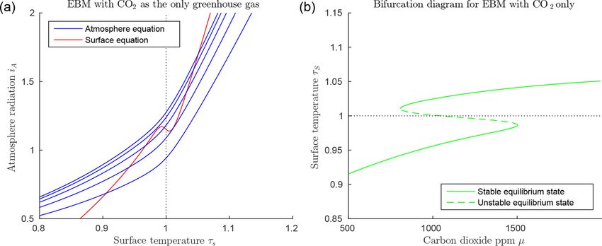
dT Figure 3a shows that the function ηW (τS ) in Eq. (34) in-
0≡− . (29)
dz creases rapidly from near 0 to near 1 as τS increases past
Normally, 0 is positive and is close to constant in value 1, and it steepens towards a step function as δ increases.
from the surface to the tropopause. The International Civil This implies that if the surface temperature τS in the surface
Aviation Organization has defined, for reference purposes, energy balance Eq. (10) increases past τS = 1, then the ab-
the ISA, in which 0 is assigned the constant value 0 = sorptivity of water vapour ηW (τS ), acting as a greenhouse
6.49×10⁻³ K m−1 (ICAO, 1993). Using this assumption, the gas in Eq. (9), increases rapidly, thus amplifying the heat-
variation in temperature with height is given as ing of the atmosphere by the radiation IS = σ TS4 from the
surface. Energy balance requires a corresponding increase
T (z) = TS − 0z or τ (z) = τS − γ z, (30) in the radiation IA transmitted from the atmosphere back
to the surface, further increasing the surface temperature τS .
where the normalized lapse rate is γ = 0/TR = 2.38 × This is a positive feedback loop called water vapour feed-
10−5 m−1 . The tropopause height Z ranges from 8 to 11 km back. This positive feedback is manifested in Fig. 3b in
at the poles and 16 to 18 km at the Equator, based on satellite the additional increase in TS on the warm branch, beyond
measurements (Kishore et al., 2006). Therefore, both T (Z) that due to the ice–albedo bifurcation. Compare this with
and τ (Z) are positive. For this paper we will take the height Fig. 2, where no water vapour is present. This rapid non-
to be Z = 9 km at the poles and Z = 17 km at the Equator. linear change is due to the relatively large size of the green-
Lv
Equation (30) may be used to change the variable of inte- house constant GW1 = RW TR = 17.89 in the exponent of the
gration in Eq. (28) for the optical depth of water vapour, from Clausius–Clapeyron Eq. (27), as it reappears in Eq. (34).
www.clim-past.net/15/493/2019/ Clim. Past, 15, 493–520, 2019502 B. Dortmans et al.: EBM for paleoclimate transitions
Figure 3. Climate EBM (Eqs. 9–10) including greenhouse effect of water vapour only, µ = 0 (with FA = 45, FO = 50, Q = 173.2 Wm−2 ,
αW = 0.08, and Z = 9 km). (a) Absorptivity ηW (τS ) as given by Eq. (34) with relative humidity δ = 0.4, 0.6 and 0.8 from bottom to top
blue lines. Below freezing (τs < 1) water vapour has little influence as a greenhouse gas, but absorptivity increases rapidly to approach η = 1
for τ > 1. (b) Bifurcation diagram for EBM with µ = 0, and relative humidity increasing from 0 to 1. Note the accelerated increase in surface
temperature τS above τS = 1, compared to that in Fig. 2b, due to the rapid increase in ηW .
2.3.4 Combined CO2 and H2 O greenhouse gases to an abrupt increase in temperature. The second is water
vapour feedback in the atmosphere equilibrium equation. As
The combined effect of two greenhouse gases is determined
shown in Fig. 3, if the surface temperature continues to in-
by the Beer–Lambert law as shown in Sect. 2.2. If ηC is the
crease above freezing, then the absorptivity of water vapour
absorptivity of CO2 as in Eq. (21) and ηW is the absorptiv-
increases dramatically, strengthening the greenhouse effect
ity of H2 O as in Eq. (28), then the combined absorptivity
for water vapour and further increasing the temperature. Both
η of these two is obtained by adding the two corresponding
of these mechanisms act independently of the concentration
optical depths λC and λW . The overall absorptivity of the at-
of CO2 itself in the atmosphere. However, if the concentra-
mosphere including these two greenhouse gases and the (as-
tion of CO2 goes up, causing a rise in temperature, then each
sumed) constant effect of clouds is, by Eq. (17),
of these two positive feedback mechanisms can amplify the
η(τS ) = 1 − (1 − ηC )(1 − ηW )(1 − ηCl ) increase in temperature that would occur due to CO2 alone.
= 1 − exp [−λC − λW (τS )] (1 − ηCl )
3 Applications of the energy balance model
= 1 − exp − µ · GC − δ GW2
The goal of this section is an exploration of the underlying
ZτS causes of abrupt climate changes that have occurred on Earth
1 τ −1
exp GW1 dτ (1 − ηCl ). (35) in the past 100 million years, using, as a tool, the EBM de-
τ τ veloped in Sect. 2. The most dramatic climate changes oc-
τS −γ Z
curred in the two polar regions of the Earth. The climate of
The full nondimensional two-layer EBM is therefore speci- the tropical region of the Earth has changed relatively little in
fied by Eqs. (9)–(12) and (35), and the parameter values in the past 100 million years. In this section, the EBMs for the
Table 1. two polar regions are applied to the Arctic Pliocene paradox,
the glaciation of Antarctica, the warm, equable Cretaceous
2.4 Positive feedback mechanisms problem and the warm, equable Eocene problem. For com-
parison, a control EBM with parameter values set to those of
The above analysis shows that there are two highly nonlinear the tropics shows no abrupt climate changes in the tropical
positive feedback mechanisms in this EBM. Both serve to climate for the past 100 million years.
amplify an increase (or decrease) in surface temperature TS
near the freezing point as follows. Consider the case of rising
3.1 EBM for the Pliocene paradox
temperature. The first feedback is ice–albedo feedback, due
to a change in albedo in the surface equilibrium equation. The Arctic region of the Earth’s surface has had ice cover
As illustrated in Fig. A1, if the surface temperature increases year-round for only the past few million years. For at least
slowly through the freezing point, causing a drop in albedo, 100 million years prior to about 3 Ma, the Arctic had no per-
there is a large increase in solar energy absorbed, leading manent ice cover, although there could have been seasonal
Clim. Past, 15, 493–520, 2019 www.clim-past.net/15/493/2019/B. Dortmans et al.: EBM for paleoclimate transitions 503
snow in the winter. Recently, investigators have found plant the Greenland ice sheet in the late Pliocene. Recently, Tan
and animal remains, in particular on the farthest northern et al. (2018) have strengthened this conclusion.
islands of the Canadian Arctic Archipelago, which demon- During the Pliocene Epoch, important forcing factors that
strate that there was a wet temperate rainforest there for mil- determine climate were very similar to those of today. The
lions of years, similar to that now present on the Pacific Earth orbital parameters, the CO2 concentration, solar ra-
Northwest coast of North America (Basinger et al., 1994; diation intensity, position of the continents, ocean currents
Greenwood et al., 2010; Struzik, 2015; West et al., 2015; and atmospheric circulation all had values close to the values
Wolfe et al., 2017). The relative humidity has been estimated they have today. Yet, in the early/mid-Pliocene, 3.5–5 mil-
at 67 % (Jahren and Sternberg, 2003), and this value has been lion years ago, the Arctic climate was much milder than that
chosen for δ in the Arctic EBM of this section. The change of today. Arctic surface temperatures were 8–19 ◦ C warmer
from an ice-free to an ice-covered condition in the Arctic than today and global sea levels were 15–20 m higher than
occurred abruptly, during the late Pliocene and early Pleis- today, and yet CO2 levels are estimated to have been 340–
tocene. This is sometimes called the Pliocene–Pleistocene 400 ppm, about the same as 20th century values (Ballan-
transition (PPT 3.0–2.5 Ma; Willeit et al., 2015; Tan et al., tyne et al., 2010; Csank et al., 2011; Tedford and Harington,
2018). It has been a longstanding challenge to explain this 2003). As mentioned in the Introduction section, the problem
dramatic change in the climate; however, significant progress of explaining how such dramatically different climates could
has been made recently for the case of the Greenland ice exist with such similar forcing parameter values has been
sheet (GIS). The authors of Willeit et al. (2015) have solved called the Pliocene paradox (Cronin, 2010; Fedorov et al.,
the “inverse problem” for the GIS by finding a schematic 2006, 2010; Zhang and Yan, 2012).
pCO2 concentration scenario from an ensemble of transient Another interesting fact concerning polar glaciation is that
simulations using an EMIC that gives the best fit to data although both poles have transitioned abruptly from ice-free
from 3.2 to 2.4 Ma, taking into account the obliquity cycle. to ice-covered conditions, they did so at very different ge-
Meanwhile, Tan et al. (2018) have used an AOGCM asyn- ological times. The climate forcing conditions of Earth are
chronously coupled with sophisticated ice sheet models to highly symmetric between the two hemispheres, and for most
reproduce the waxing and waning of the GIS across the PPT, of the past 200 million years (or more) the climates of the
obtaining good qualitative agreement with ice rafted debris two poles have been similar. However, there was an anoma-
data reconstructions. lous interval of about 30 million years, from the EOT, 34 Ma,
Currently, there is great interest in the mid-Pliocene cli- to the early Pliocene, 4 Ma, when the Antarctic was largely
mate, because it is the most recent paleoclimate that resem- ice covered but the Arctic was largely land ice free. Because
bles the future warmer climate now predicted for the Earth. CO2 disperses rapidly in the Atmosphere, its concentration
Significant progress in understanding the Pliocene climate µ must be the same everywhere at any given time. Therefore
has been achieved in recent years. The Pliocene Research, we seek a forcing factor other than µ to account for this 30-
Interpretation and Synoptic Mapping (PRISM) project of the million-year period of broken symmetry. One obvious differ-
US Geological Survey has contributed to this goal (Dowsett ence is geography. Since the Eocene, the South Pole has been
et al., 2011, 2013, 2016), as has the Pliocene Model Inter- land-locked in Antarctica, while the North Pole has been in
comparison Project (PlioMIP; Haywood et al., 2011, 2016; the Arctic Ocean. Therefore, our two EBMs for the North
Zhang et al., 2013). Advances in the extraction and inter- Pole and South Pole have very different values for ocean heat
pretation of proxy data have given a clearer picture of the transport FO . We will show that this difference is sufficient to
warm Pliocene climate (Haywood et al., 2009; Salzmann account for the gap of 30 million years between the Antarctic
et al., 2009; Ballantyne et al., 2010; Steph et al., 2010; Seki and Arctic glaciations.
et al., 2010; Bartoli et al., 2011; De Schepper et al., 2013; Our Pliocene Arctic EBM brackets the Pliocene Epoch
Knies et al., 2014; O’Brien et al., 2014; Brierley et al., 2015; between the mid-Eocene (50 Ma) and pre-industrial mod-
Fletcher et al., 2018). At the same time, computer models ern times, and it models the effects of the slow decrease in
have achieved closer agreement with proxy data, see for ex- both CO2 and ocean heat transport FO in the Arctic over this
ample Haywood et al. (2009); Dowsett et al. (2011); Zhang long time interval. In this Arctic model, abrupt glaciation of
and Yan (2012); Sun et al. (2013); Willeit et al. (2015); Tan the Arctic is inevitable, due to the existence of a bifurcation
et al. (2017, 2018); Chandan and Peltier (2017, 2018), and point.
other references therein. Using a fully coupled atmosphere– During the Eocene (56–34 Ma), temperatures were much
ocean GCM, Lunt et al. (2008) considered the following higher than today, especially in the Arctic (Greenwood et al.,
forcing factors contributing to late Pliocene glaciation: de- 2010; Wolfe et al., 2017; Huber and Caballero, 2011); also,
creasing carbon dioxide concentration, closure of the Panama CO2 concentration µ was higher than today. Estimates of
seaway, end of a permanent El Niño state, tectonic uplift Eocene CO2 concentration µ vary from 1000–1500 ppm (Pa-
and changing orbital parameters. They concluded that falling gani et al., 2005, 2006) to 490 ppm (Wolfe et al., 2017).
CO2 levels were primarily responsible for the formation of For this EBM, we set mid-Eocene CO2 at µ = 1000 (Pagani
et al., 2005). Both temperature and CO2 concentration have
www.clim-past.net/15/493/2019/ Clim. Past, 15, 493–520, 2019504 B. Dortmans et al.: EBM for paleoclimate transitions
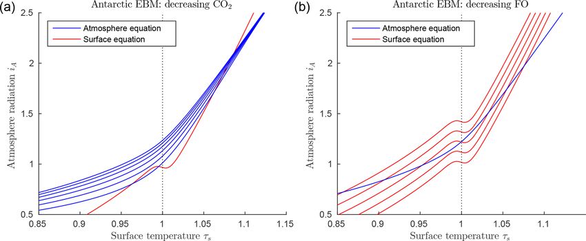
decreased steadily but not monotonically, with many fluc- Figure 4a shows graphs of the surface and atmosphere
tuations from their Eocene values to pre-industrial modern equilibrium equations for the Arctic Pliocene EBM, for vary-
values. The overall decrease in CO2 concentration observed ing values of µ. The figure shows only one surface equilib-
since the Eocene may be attributed to decreased volcanic ac- rium curve (red), with FO = 50 W m−2 , because the change
tivity, increased absorption and sequestration by vegetation in FO is relatively small. The blue atmosphere equilibrium
and the oceans, continental erosion, and other sinks. curves represent values of CO2 concentration µ falling from
The changes in ocean heat transport to the Arctic are more 1100 to 200 ppm, from the top to bottom blue curves. It is
complicated and derive from many factors only summarized clear that there may exist up to three points of intersection of
here (De Schepper et al., 2015; Haug et al., 2004; Knies et al., a given atmosphere equilibrium curve (blue) with the sur-
2014; Lunt et al., 2008; Zhang et al., 2013). There was a face equilibrium curve (red); namely, a warm equilibrium
slow drop in global sea level, in large part due to the grad- state τs > 1, a frozen equilibrium state τS < 1 and a third (in-
ual accumulation of vast amounts of water in the form of termediate) solution, which is always unstable (when it ex-
ice and snow on Antarctica. It has been estimated that the ists). As µ decreases and the warm equilibrium state τs > 1
total amount of ice today in the Antarctic is equivalent to approaches the local minimum on the red S-shaped curve,
a change in sea level of about 58 m (Fretwell et al., 2013; the unstable intermediate equilibrium state moves down the
IPCC, 2013). This drop in sea level likely reduced the flow of middle branch of the red S-shaped curve. When they meet,
warm tropical ocean water into the Arctic. Against this back- these two equilibria coalesce, then disappear, via a saddle-
ground, several other factors came into play due to chang- node bifurcation. Beyond this saddle-node bifurcation, only
ing geography. In the Eocene, the North Atlantic Ocean was one equilibrium state remains, which is the stable frozen
not always connected to the Arctic, but the Turgai Sea ex- state on the left in the Figure. Dynamical systems theory
isted between Europe and Asia and connected the warm In- tells us that following this bifurcation, the system will transi-
dian Ocean to the Arctic, until about 29 Ma (Briggs, 1987). tion rapidly to that frozen equilibrium state. The paleoclimate
By the Oligocene, the Turgai Sea had closed and the North record shows that CO2 concentration was trending downward
Atlantic had opened between Greenland and Norway, form- for millions of years before and during the Pliocene. There-
ing a deep-water connection to the Arctic Ocean. The Bering fore, Fig. 4a predicts that an abrupt drop in temperature to
Strait opened and closed. During the Pliocene the formation a frozen state would be inevitable if this trend continued far
of the Isthmus of Panama about 3.5 Ma cut off a warm equa- enough.
torial current that had existed between the Atlantic and Pa- In order to explore this downward trend further, we bracket
cific, at least since Cretaceous times. On the Atlantic side the Pliocene Epoch between the mid-Eocene Epoch (50 Ma)
of the isthmus, the sea water became warmer, and became and the pre-industrial modern era (300 years ago), and define
more saline due to evaporation. The Gulf Stream carried this a surrogate time variable ν by
warm salty water to western Europe. One might expect the
Gulf Stream to transport more heat into the Arctic. How- t = 50(1 − ν) Ma. (36)
ever, some believe that the Gulf Stream actually contributed
to glaciation in the Arctic (Haug et al., 2004; Bartoli et al., As reviewed above, it is believed that ocean heat transport
2005) as follows. Evaporation from the Gulf Stream waters FO decreased modestly over this time period, mainly due to
contributed to rainfall across northern Europe and Siberia, the drop in global sea level, while the CO2 concentration µ
increasing the flow of fresh water in rivers emptying into decreased more significantly. Therefore, we express both µ
the Arctic Ocean. This reduced the salinity, and hence the and FO as decreasing functions of bifurcation parameter ν
density, of the Arctic Ocean waters. The Gulf Stream wa-
ters in the North Atlantic now cooler, and denser due to high µ = 1000 − 730 · ν ppm
salinity, were forced downward by the less dense Arctic wa- FO = 60 − 10 · ν Wm−2 . (37)
ters, which began to flow into the North Atlantic on the sur-
face. The denser Gulf Stream waters returned southward as Here, ν = 0 corresponds to estimated mid-Eocene values of
a deep ocean current, without having conveyed much heat to µ and FO (Pagani et al., 2005; Wolfe et al., 2017; Bar-
the Arctic. Meanwhile the low salinity Arctic surface water, ron et al., 1981), while ν = 1 corresponds to modern pre-
with a higher freezing temperature, began to freeze, resulting industrial values (IPCC, 2013). Equation (37) defines µ and
in higher albedo and accelerating Arctic glaciation. In large FO as linear functions of ν. In the real world, neither µ nor
measure, these changing geographical factors partially can- FO decreased linearly. This is not an obstacle for our bifurca-
celled each other in their contributions to ocean heat trans- tion analysis. What is important is that, somewhere between
port to the Arctic. In the EBM, we summarize all of the above ν = 0 and ν = 1, a bifurcation point is crossed.
heat transport mechanisms by specifying a slow overall de- Figure 4b is a bifurcation diagram, which shows the de-
crease in ocean heat transport to the Arctic, represented by pendence of surface temperature τS on this bifurcation pa-
the single forcing parameter FO . rameter ν. Note that for ν = 0 (mid-Eocene values, 50 Ma)
only the warm equilibrium state exists. At about ν = 0.116
Clim. Past, 15, 493–520, 2019 www.clim-past.net/15/493/2019/You can also read