REDDIT'S SELF-ORGANISED BULL RUNS: SOCIAL CONTAGION AND ASSET PRICES - MUNICH PERSONAL REPEC ...
←
→
Page content transcription
If your browser does not render page correctly, please read the page content below
Munich Personal RePEc Archive

Reddit’s self-organised bull runs: Social
contagion and asset prices

Semenova, Valentina and Winkler, Julian

Institute of New Economic Thinking at the Oxford Martin School,
Department of Mathematics, University of Oxford, Department of
Economics, University of Oxford

5 May 2021

Online at https://mpra.ub.uni-muenchen.de/107575/
MPRA Paper No. 107575, posted 08 May 2021 07:29 UTC
Reddit’s self-organised bull runs: Social contagion and asset
                                                        prices
                             Valentina Semenova*1,2 and Julian Winkler†1,3
                  1 Institute  of New Economic Thinking at the Oxford Martin School
                            2 Department of Mathematics, University of Oxford
                             3 Department of Economics, University of Oxford

                                                    May 5, 2021‡

                                                        Abstract

          This paper develops an empirical and theoretical case for how ‘hype’ among retail investors can
      drive large asset fluctuations. We use the dataset of discussions on WallStreetBets (WSB), an online
      investor forum with over nine million followers as of April 2021, to show how excitement about
      trading opportunities can ripple through an investor community with large market impacts. This
      paper finds empirical evidence of psychological contagion among retail investors by exploiting
      differences in stock price fluctuations and discussion intensity. We show that asset discussions on
      WSB are self-perpetuating: an initial set of investors attracts a larger and larger group of excited
      followers. Sentiments about future stock performance also spread from one individual to the next,
      net of any fundamental price movements. Leveraging these findings, we develop a model for how
      social contagion impacts prices. The proposed model and simulations show that social contagion
      has a destabilizing effect on markets. Finally, we establish a causal relationship between WSB
      activity and financial markets using an instrumental variable approach.
          JEL codes: D91, G14, G41.

    Acknowledgements
    We thank Rick Van der Ploeg, J. Doyne Farmer, Xiaowen Dong and Steve Bond for supervising this research. We are
grateful to Francis DiTraglia, Kevin Sheppard, Marteen Scholl, John Pougué-Biyong, Ilan Strauss, Jangho Yang, Torsten
Heinrich, François Lafond, Matthias Winkler, José Moran, Farshad Ravasan, Mirta Galesic, Renaud Lambiotte and partic-
ipants of the Royal Economic Society annual conference for their helpful comments and insightful questions. We thank
Baillie Gifford and the Institute for New Economic Thinking at the Oxford Martin School for funding our work at the
University of Oxford.
   * valentina.semenova@maths.ox.ac.uk
  † julian.winkler@economics.ox.ac.uk
  ‡ First version uploaded online January 20th , 2021

                                                           1
1 Introduction
A trite yet fundamental question in economics is: What causes large asset price fluctuations? A ten-
fold rise in the price of GameStop equity, between the 22nd and 28th of January 2021, demonstrates
that herding behaviour among retail investors is an important contributing factor. On this occasion,
thousands of retail investors launched a speculative attack on the short positions held in GameStop
by hedge funds, using social media as their coordination platform.
As academics and regulators alike grapple with the implications, many wonder whether large-
scale coordination among retail investors is the new ‘modus operandi’, or a one-off fluke. We argue
that this is a new manifestation of a well-established global phenomenon. Social media has changed
the fabric of society. Polarization, the spread of fake news and other societal challenges are some of its
documented consequences (Tucker et al. 2018). 4.2 billion people, or 53.6% of the world population,
are active social media users, each just a few clicks away from the next popular phenomenon.1 Now,
a growing audience turns to social media for promising stock market gambles.
To the extent that humans are a social species, personal interactions are likely to play a role in
financial decision-making. Consider, for example, that many bank runs (such as the Japanese finan-
cial crisis in 1927 or the Swedish bank run of 2011) have been triggered by a simple rumour. Studies
of social dynamics in stock market activity date back to Shiller (1984), a seminal paper reminding
us that ‘investing in speculative assets is a social activity.’ Internet communities are simply conduits,
enabling retail investors to come together at an unprecedented scale.
Nevertheless, we lack a holistic theory, backed by empirical evidence, for how social interactions
drive investment decisions. Practical difficulties and lack of data have restricted many researchers
to controlled laboratory experiments, whose external validity remains unchecked. The new invest-
ing climate, enabled by communications technology, offers both an extraordinary opportunity and
urgent need to understand the role that social dynamics play.
This paper sets out to reconcile the extreme nature of the behaviours on social media with eco-
nomic theory. We use text data from the ‘WallStreetBets’ (WSB) Reddit forum to gain insight into
investor social dynamics. Reddit is a social news aggregation site, ranked 19th most visited website
in the world, as of April 2021.2 Reddit, and WSB more specifically, have several desirable features
for this line of research. The WSB forum is completely anonymous, with the quality of content alone
driving further discussion. Users try to garner a following by galvanising their peers with their bal-
looning balances and precipitous losses, which they avidly post online. Finally, WSB has gained a
colossal following: the forum currently has over nine million self-described ‘degenerates’.3 Putting
these numbers into perspective, The Times newspaper recently boasted 7.5 million subscriptions.4
We first document evidence of social contagion on the forum. The working hypothesis is that
users’ expressed interest in assets depends on the discussions they engage with. Demand, much
like an epidemic, ‘dies out’ if the asset is not discussed. Accurately evaluating contagion from one
interested user to another is not straightforward due to endogeneity (Aral et al. 2009). This issue
is addressed with a two-fold approach: i) a panel regression, controlling for outside factors, and ii)
an opinion dynamics model that matches users on observable characteristics. The results demon-
strate significant contagion in asset demand after accounting for endogeneity. Users who comment
on discussions about an asset are between four and nine times more likely to subsequently start a
new conversation about the asset themselves, compared to their matched counterparts in the control
group.
The next question is whether investment strategies also transmit between users: in other words,
2AMD MU
6
Billions of USD
4
2
0
−2
2016 2017 2018 2019 2020 2016 2017 2018 2019 2020
De−meaned Trading Volume Prediction from WSB Activity
Figure 1: Hype-Driven WSB Activity and Trading Volumes; the predicted number of new users
interested in a ticker, for a given week, correlates strongly with observed weekly trading volumes
for AMD (Advanced Micro Devices) and MU (Micron Technology). Both series are plotted as four week
rolling moving averages. See Section 4.4 for details.
whether we observe consensus. We measure ‘buy’ versus ‘sell’ strategies via the expressed sentiment
about future asset performance in WSB submissions. The spread of sentiments about an asset can
be measured by the associated spillover from the network of discussions. This network links sub-
missions by their authors’ comments to older submissions mentioning the same asset. The results
indicate that sentiments in submissions correlate strongly and significantly with the sentiments of
neighbours, especially for bearish posts; the submission from a user who commented on a bearish
post in the past is almost 50% more likely to be bearish than indifferent, net of market factors. Social
interactions thus play an important role in determining investor sentiment. The asymmetry of the
transmission mechanism of bullish versus bearish sentiment is of particular interest. Despite users
encouraging risk-taking, there is strong evidence for risk-aversion and panic selling.
After characterizing the nature of social dynamics, a crucial question remains: what are the im-
plications for financial market stability? Some may argue that the key dynamics, contagion and con-
sensus, could lead to the fast spread of news and quick price convergence to an asset’s ‘true’ market
value. Others may consider the potential for unchecked rumours to permeate the investor commu-
nity, driving the market to diverge from fundamentals and to exhibit greater volatility.
In order to tackle this question, we propose a simple model with two mechanisms through which
social dynamics impact asset prices: i) ‘contagion’, which generates the hump-shaped pattern in de-
mand for an asset over time, as new investors initially buy into the hype but eventually become unin-
terested in an asset, and ii) ‘consensus’, which captures the extent of coordination in buying/selling
amongst these investors. We borrow from Shiller (2017) to describe the rise and subsequent fall in
investor interest. A discrete time simulation of our model, based on parameters initiated from WSB
data, demonstrates that assets experience an initial, slow rise in value followed by a crash and period
of high volatility.
We validate the existence of a causal link between WSB activity and the stock market through a
Two-Stage-Least-Squares approach. We predict new users discussing an asset on WSB using histori-
cal WSB and market data: these new users are ‘hype’ investors, driven to join the trading activity by
the excitement of their peers rather than by news or fundamentals. The predicted number of new
3authors, plus the lag in average sentiment, are fitted to data on price returns, volatility, and trading
volumes, after removing temporal and cross-sectional means. Our key finding is that our instru-
mental variable performs particularly well in explaining asset trading volumes. Figure 1 displays
this result for two heavily discussed stocks, namely Advanced Micro Devices (AMD) and Micron
Technology (MU). Hype investors appear cyclical: interest, built up over several weeks, eventually
fades out. Their activity is correlated to negative asset returns and higher volatility. These findings
offer empirical evidence of the fact that the bull runs generated by WSB activity are destabilising.
The next section comprehensively describes the data source and relevant variables. Section 3
brings to light empirical evidence of investor social dynamics. Section 4 presents a behavioural
model for how asset interest and sentiments spread among investors, with implications for asset
prices. It presents a causal relationship between WSB activity and market variables. Section 5 con-
cludes.
2 What is WallStreetBets?
105
Daily Frequency, 30−Day MA
104
103
102
101
100
2013 2014 2015 2016 2017 2018 2019 2020
Submissions Comments
Figure 2: Daily Activity on WSB Plotted on a Logarithmic Scale; the daily submission and comment
counts, averaged over 30 days, demonstrate a persistent exponential increase from 2015 to 2020, with
a substantial jump in early 2020.
Reddit, launched in 2005, is a social news aggregation, web content rating, and discussion web-
site. It was ranked as the 19th most visited site globally in April 20215 , with over 430 million anony-
mous users by the end of 20196 . The website’s contents are self-organized by subject into smaller
sub-forums, ‘subreddits,’ to discuss a unique, central topic.
Within subreddits, users make titled posts (also called submissions), typically accompanied with
a body of text or a link to an external website. These submissions can be commented and upvoted or
downvoted by other users. A ranking algorithm raises the visibility of a submission with the amount
of upvotes it receives, but lowers it with age. Therefore, the first posts that visitors see are i) highly
upvoted, and ii) recent. Comments on a post are also visible, are subject to a similar scoring system,
and can, themselves, be commented on.
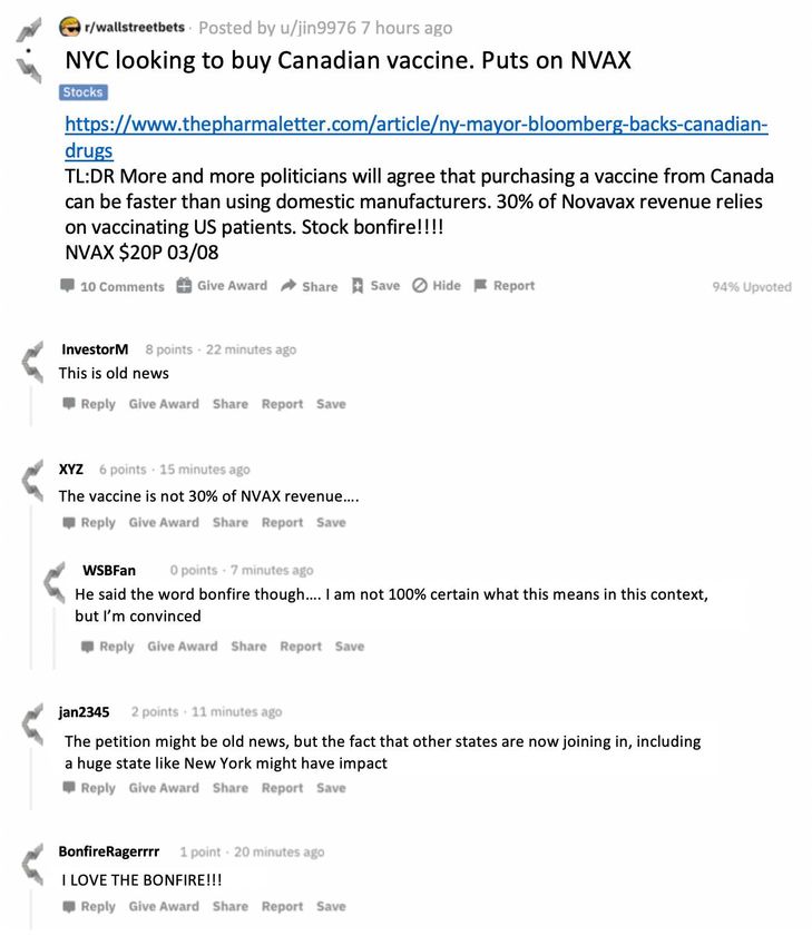
4(a) A Typical Discussion on WSB (b) A Sample Screenshot of User Profits
Figure 3: What Does WSB Look Like? These snapshots exemplify typical discussions on WSB. The
exact text, usernames, and conversation details have been modified to protect user identities.
The WSB subreddit was created on January 31, 2012, and reached one million followers in March
20207 . As per a Google survey from 2016, the majority of WSB users are ‘young, male, students that
are inexperienced investors utilizing real money (not paper trading); most users have four figures
in their trading account’8 . The conversation guidelines outlined by the moderators of WSB handily
demonstrate the financial focus and whimsical tone of discussions:9
• Discussion about day trading, stocks, options, futures, and anything market related,
• Charts and Technical Analysis,
• Shower before posting,
• Some irresponsible risk taking,
• People sharing trades, ideas, observations.
We gain insight into the content of WSB discussions through a biterm topic model (Yan et al.
2013). The model detects a mix of conversations, from those that follow specific real world trends,
such as the China trade war or the COVID-19 pandemic, to those that hype positions on a hand-
ful of stocks and indices, most famously the GameStop (GME) short squeeze. Some topics persist
across time: people consistently ask for advice about trading accounts and anonymously share de-
tails of how their trading is affecting their personal lives. On the other hand, topics concerned with
specific economic interests wax and wane. Two examples of this are the uptick in submissions dis-
cussing GME and Robinhood account trading limits, coinciding with the GME short squeeze, and
the COVID-19 topic, which is negligible until January 2020, but gains prominence in the subsequent
months. A full description of the topic model and the temporal trends of topics are presented in
Appendix A.8.
The subreddit’s size grew exponentially since 2015, plotted in Figure 2. Two jumps are notable:
a smaller, seemingly idiosyncratic rise in early 2018, and a sharp spike during the COVID-19 pan-
demic. Figure 3a displays a typical exchange on the WSB forum: individuals discuss stock-related
5news and their sentiments on whether this will affect stock prices in the future. In addition to market
discussions, there is ample evidence of users pursuing the investment strategies encouraged in WSB
conversations. Users post screenshots of their investment gains and losses, which moderators are
encouraged to verify, as illustrated in Figure 3b. These observations are reminiscent of Shiller (2005)
in his definition of an asset bubble as:
A situation in which news of price increases spurs investor enthusiasm which spreads
by psychological contagion from person to person, in the process amplifying stories that
might justify the price increases and bringing in a larger and larger class of investors,
who, despite doubts about the real value of an investment, are drawn to it partly through
envy of others’ successes and partly through a gambler’s excitement.
All posts made on Reddit, plus their metadata, can be queried via Reddit’s API, as well as other
sources. In what follows, we downloaded data on WSB using the PushShift API10 . The only caveat of
PushShift is that all data are recorded at the time of posting.
The full dataset consists of two parts. The first is a total of 452,720 submissions, with their au-
thors, titles, text and timestamps. The second is comprised of 15.4 million comments, with their
authors, text, timestamp, and their linked comment or post. The following sections will predomi-
nantly rely on submissions for text data, since they are substantially richer. Comments are largely
used to trace user activity and, subsequently, the interaction between discussants. User submissions
data, external to WSB, is also downloaded from PushShift, but is only available through April, 2020.
The availability of external user data forces us to rely on data until April 30th , 2020 for our analysis,
unless otherwise specified.
2.1 Identifying Asset Discussions
In order to understand how users discuss specific assets, we extract mentions of ‘tickers’ from the
WSB submissions text data. A ticker is a short combination of capital letters, used to identify an
asset in the financial markets. For example, ‘AAPL’ refers to shares in Apple, Inc. Appendix A.1
documents how tickers are extracted from submissions. Table 7 in Appendix A.1 displays the twenty
tickers that feature most prominently in WSB conversations. These are typically shares in technology
firms, such as AMD or FB. A handful of indices are also present, notably the S&P 500 (SPY) and a
gold ETF (JNUG).
A small fraction of the 4,650 tickers we extract dominate the discourse on WSB. 90% of tickers
are mentioned fewer than 31 times, and more than 60% are mentioned fewer than five times. The
frequency distribution of tail of ticker mentions demonstrates this point, for which Figure 4 displays
a QQ-plot. We arbitrarily selected tickers with the number of mentions in the top 10th percentile.
Even though threshold of mentions for this top decile is 30 subsmissions, the most popular, SPY,
features in almost 8,000 submissions. The orange crosses in Figure 4 locate the empirical densities,
on a log scale, which are plotted against the theoretical quantiles of an exponential distribution
on the x-axis. Under the assumption that ticker mentions are heavy-tailed (similarly to vocabulary
distributions), the logarithm of the mentions follows an exponential distribution, with the intercept
at the threshold, and the slope equal to the inverse of the tail index. Indeed, the linear fit is close
to perfect, supporting the assumption that the popularity of assets in WSB is heavy-tailed, with an
estimated tail exponent of approximately 1.03. In what follows, we used submissions for which we
identified a single ticker, unless otherwise specified, forming a dataset of 103,205 submissions with
unique ticker mentions by our cutoff date.
6104 Slope = 0.975
Intercept = 3.43
Implied tail index: 1.03
Log−data 103
102
0 2 4 6
Theoretical Quantiles of Exponential
Figure 4: QQ Plot of the Tail in Ticker Mentions on WSB; the number of submissions for each ticker
(on a log-scale) is plotted against the theoretical quantiles of an exponential distribution. Quantiles
are calculated as q(i) = − log(1 − i/(N + 1), where N is the number of observations, and i the order
of the statistic, from 1 to N . The linear fit suggests that the data follows a Pareto distribution, with
the tail index equal to the inverse of the slope. The threshold for a ticker to be part of the ‘tail’ is 31
mentions; note the intercept, at exp(3.43) ≈ 31.
2.2 Sentiments about Assets
In order to thoroughly understand the social dynamics of asset discussions, it is not sufficient to
simply identify what assets are being discussed, as in Section 2.1; it is important to understand
what is being said about them. Our goal, with regards to the text data in WSB, is to gauge whether
discussions on certain assets express an expectation for their future price to rise, the ‘bullish’ case, to
fall, the ‘bearish’ case, or to remain unpredictable, the ‘neutral’ case.
A series of studies link sentiment, measured through diverse approaches, to stock market per-
formance (Garcia 2013, Tetlock 2007, Bollen et al. 2011). Gentzkow et al. (2019) offer a thorough
review. Many of these works use lexicon approaches, whereby documents are scored based on the
prevalence of words associated with a certain sentiment. Recently, machine learning has offered al-
ternative, powerful tools, such as Google’s Bidirectional Encoder Representations from Transformers
(BERT) algorithm (Devlin et al. 2018). The BERT algorithm trains a final layer of nodes in a neural
network from a pre-trained classifier on labelled data. The classifier itself is a neural net, pre-trained
by Google on a corpus of Wikipedia entries to i) predict the probability distribution of words ap-
pearing in a given sentence (Masked Language Modeling), and ii) predict the relationship between
sentences (Next Sentence Prediction).
Among other alternatives, we pursued a supervised-learning approach to identify the sentiment
expressed about an asset within a WSB submission. This required a training dataset, for which
we manually labelled 2,581 random submissions with unique ticker mentions as either ‘bullish,’
‘bearish’ or ‘neutral,’ with respect to the authors’ expressed expectations for the future price. We
used the BERT algorithm for labeling. Work not shown here implements an alternative regression-
based approach as a robustness check, but BERT performs better out-of-sample. We discuss BERT’s
7results and accuracy in Appendix A.2.
3 Social Dynamics among Retail Investors: Evidence of Contagion and
Consensus
Do investors express demand for an asset because of an independently perceived payoff, or because
of another investor’s stated interest? The endogenous dynamics in the WSB community can be esti-
mated as a spillover rippling through a network of people, linked by their interactions on WSB.
Section 3.1 quantifies the spread in asset interest through the WSB network. It pursues a two-
fold approach: i) a regression estimating the probability of current discussants of an asset to attract
a greater following, and ii) matching on observables, outlined in Leng et al. (2018), Lehmann &
Ahn (2018), in order to estimate a causal link between a user’s engagement with a stock and their
future posting activity on that ticker. Both approaches attempt to mitigate the problems arising from
homophily in endogenous link formation in networks, discussed in Aral et al. (2009).
Section 3.2 studies consensus among investors: if a user engages in a discussion about an asset
with an expressed sentiment, what is the probability they adopt the same sentiment? The evolu-
tion of collective dynamics on social networks are studied in many contexts, including healthcare
outcomes and product adoption, among others (Christakis & Fowler 2008, Lehmann & Ahn 2018).
Their methodology builds a logistic regression model for the dependent variable at time t + 1 as a
function of demographic attributes and the status of the dependent variable among contacts at time
t. This paper pursues a similar approach as it is a fruitful, simple way to gain an estimate of peer
influence The results demonstrate that the WSB network exhibits significant sentiment contagion, as
older submissions influence future sentiments, to the degree that users interact.
3.1 Contagion in Asset Demand
Total Users 600
Number of Active Users on WSB
40000
TSLA
500
Number of Users Posting
MU
about Specified Ticker
30000 JNUG 400
RAD
300
20000
200
10000
100
0 0
2013 2014 2015 2016 2017 2018 2019 2020
Figure 5: Ticker Activity versus Overall WSB Activity; the number of unique monthly active users
(users who comment or post) on the left y-axis plotted against the unique number of posters about a
specific ticker (on the right y-axis). Both are plotted as 3-month rolling means.
This section sets out to demonstrate empirically that asset interest, among investors on the WSB
forum, is subject to contagion. Figure 5 shows how stock discussions permeate the forum for a
8select subset of popular stocks: we plot the three-month rolling average of the number of unique
authors who post about a specific ticker. Visually, an initial group of users appears to attract a larger
following. Eventually, interest is a specific asset dissipates, as users turn to new opportunities. Such
behaviour is reminiscent of a Kermack-McKendrick Susceptible-Infected-Recovered (SIR) epidemic
model, proposed for the economic context in Shiller (2017).
First, we perform a least-squares regression analysis to isolate the impact that discussions on the
forum have on begetting further discussions. We find that conversations on WSB indeed have an
endogenous component, which lends credibility to the fact that social contagion plays a role in asset
interest. Second, we perform a matching on observables exercise both to validate our initial results,
and isolate a mechanism through which contagion occurs.
Table 1: Time Dynamics of Assets Discussed on WSB
Dependent variable: ∆Ai,t
(1) (2) (3)
Ai,t−1 0.40∗∗∗ (0.002) 0.40∗∗∗ (0.002) 0.38∗∗∗ (0.002)
P3
j=1 Ai,t−j −0.06∗∗∗ (0.001) −0.06∗∗∗ (0.001) −0.06∗∗∗ (0.001)
Rei,t −1.07∗∗ (0.47)
σi,t 11.64∗∗∗ (0.34)
Qi,t 0.48∗∗∗ (0.01)
α 0.15∗∗∗ (0.01) −0.002 (0.01) −0.01 (0.01)
Model Pooled Within-week Within-week
N 118,024 118,024 116,326
Adjusted R2 0.49 0.48 0.51
∗ pwe evaluate the effect using a panel framework, controlling for exogenous variables and temporal
shifts. Our model of choice is an Ordinary Least Squares (OLS) regression:
3
X
∆Ai,t = α + cAi,t−1 − r Ai,t−j + β ′ Xi,t + εi,t , (1)
j=1
where ∆Ai,t is a measure for the number of new users who post a submission on asset i within
P
calendar week t; Ai,t−1 is the stock of existing users; Tj=1 Ai,t−j is the cumulative stock of users; Xi,t
is a vector of controls; εi,t is an error term. We find the number of existing users, Ai,t−1 , by counting
the number of unique authors who posted a submission on asset i between weeks t − 3 and t − 1. We
P
calculate the cumulative stock of users, Tj=1 Ai,t−j , by summing Ai,t−j s, from an assumed starting
point j = 3 to j = 1. Our cumulative stock of users proxies the total amount of coverage the ticker
has received in the last three weeks; we expect the number of new users to decline as this cumulative
stock increases. We experiment with different time horizons and observe that our results remain
largely unchanged; we choose to use three weeks of data to predict activity in the following week
based on the observation that ticker discussions evolve over several months, as shown in Figure 5. In
order to get reasonable coverage, we restrict ourselves to tickers mentioned over 30 times, coinciding
with the tail tickers in Figure 4.
The key results are displayed in Table 1, estimating the coefficients from Eq. 1. We observe
that enthusiasm about a ticker spreads from one user to the next. This effect is reflected by the
estimate for coefficient c. The estimated coefficient r, on the other hand, proxies for the fact that,
eventually, the set of new users who could become interested in a given asset is depleted, while
current discussants move onto the next exciting stock. c and r can be likened to the ‘contagion
rate’ and ‘recovery rate’ within the epidemiological SIR model: as more people get infected, they
will infect others (captured by positive c), however, as individuals recover, the population becomes
immune (captured by a negative r). The coefficients are statistically significant across all variants
of our model. We also find an adjusted R2 value of approximately 0.5 for all constructions of our
model. Almost half of the variance in the number of new authors is explained by our two contagion
variables.
Let us consider the implications of the most basic construction of the model, presented in column
(1). If ten authors posted a submission on asset i in the preceding week (t − 1), the model estimates
that four new authors post their own submission on the same asset in the subsequent week (t). Now
consider a similar scenario, differing only in the fact that 50 different authors post about the asset
two weeks before (at t − 2). Our model would now estimate that 18 new authors emerge: calculated
as 0.40 × 60 − 0.06 × 110 + 0.15. In the latter case, the model captures that, despite the high number
of authors currently involved in the ticker discussion, the conversation is potentially on a decline.
Column (2) addresses an important problem concerning the assumption of a fixed population of
users. Clearly, the number of users, seen in Figure 2, is anything but fixed. To account for this time
pattern, we calculate the within-week deviations of all variables, by subtracting their cross-sectional
averages in each week t. This procedure is identical to introducing week dummies, or time fixed
effects. Column (2) demonstrates that the coefficients are entirely robust, with the exception of the
constant, which turns insignificant.
In the column (3), we are interested in controlling for the stock market behaviour of asset i. It
is entirely plausible that users create new submissions to discuss i’s large returns, large volatility, or
large trading volume in week t. To control for these patterns, we introduce the average excess rate of
return in week t, Rei,t , the average standard deviation in the excess rate of return, σi,t , and the average
10dollar volume of shares traded in billions of USD, Qi,t , using data from The Center for Research on
Security Prices (CRSP). We detail the computation of each variable in Appendix A.3. Each of these
controls is again expressed in terms of deviations from weekly averages across assets. Indeed, all are
significant in explaining the number of new authors, but the improvement in R2 is marginal. The
surprising finding is that the relationship between new authors and average price returns appears
negative. Our parameters of interest, c and r, remain largely unchanged.
Identifying the Contagion Mechanism: Matching on Observables According to Table 1, asset
discussions indeed seem to have an endogenous component. However, can WSB lend us more insight
into the transmission mechanism from one passionate investor the next?
In order to validate our earlier result, we measured the propensity for a user to post a submission
about a ticker, conditional on them previously commenting on submissions discussing the same
ticker. The main challenge comes in addressing the network’s endogenous link formation, as hidden
characteristics will determine a user’s choice to comment. This problem, known as ‘homophily’ in
the broader network literature, leads to an overestimated spillover (Aral et al. 2009). We address this
issue by matching on observable user characteristics. We filter the sample of submissions to the top
one percent of tickers (top percentile tickers), by number of mentions, for this portion of our study.
Individuals who commented on a top percentile ticker submission form the treatment group, and are
matched to users who did not comment, the control group.
One important form of homophily to control for is individuals’ exposure to movements in the
asset price: one may take interest in a stock because it experiences outsized returns, rather than
hearing about it from someone else. To tackle this, we matched individuals who commented on a
submission with those who did not comment, but were active on the forum shortly after the submis-
sion was made. This effectively controls for exposure to the same market environment, as well as
associated news. In order to control for overall behavioural patterns, we matched individuals based
on similar posting and commenting patterns, and on similar activity times on WSB. Lastly, to en-
sure the most accurate match, we consider individual’s interests in other subreddits, and match with
those who share similar interests. Appendix A.4 offers further details on the distance measures used
to compare users.
Following complex contagion theory, the spread of interests and beliefs may require multiple
sources of activation, or social reinforcement (Lehmann & Ahn 2018). In order to quantify the level
of social reinforcement necessary to drive a transmission in interest, users were grouped for every
ticker by their commenting frequency on submissions related to that ticker. About 90% of users
commented on fewer than five different submissions about a specific ticker; we, therefore, grouped
together those who commented on five or more submissions. We matched each group separately to
different control groups. Regardless of the number of submissions they commented on, we do not
include commenters on the same ticker in any control groups for that ticker. Henceforth, we consider
the number of distinct submissions that an individual commented on, prior to their submission,
the amount of treatment this individual received. This effectively yields five treatment groups, for
people who commented on one, two, three, four, or over five different submissions. These categories
are plotted on the bottom of Figure 6.
The result of interest is the difference in the observed proportion of submissions in the treatment
and control groups, πjT − πjC , where
1116
14
contr ol
12
10
− π̂
(%)
tr eatment
8
6
π̂
4
2
0
1 2 3 4 5+
71%
13%
5% 6%
2%
1 2 3 4 5+
Number of Posts Commented on in Treatment Group
Figure 6: Estimated Effect of Commenting on Posting a New Submission; the distribution of the
estimated treatment effect (π̂jT − π̂jC ) across the top one percent of tickers is graphed as a series of box
plots. The solid line connects the median estimate, and the protruding dashes represent the 5th and
95th percentiles. The histogram below shows the proportion of individuals who comment between
one and over five times on a submission for a given ticker before either creating a post themselves,
or losing interest.
πjT = E(πi,j,t+T = 1|li,j,t = 1),
πjC = E(πi,j,t+T = 1|li,j,t = 0),
and πi,j,t+T is one if user i posts a novel submission on asset j at some time t + T , and li,j,t is one
if user i previously commented on a submission about asset j at time t. li,j,t is only observed once
for each individual i. Therefore, we constructed the counterfactual, π̂jC , from users matched to the
commenters based on observable characteristics. The difference π̂jT − π̂jC thus measures the likeli-
hood a user will post a submission given they are exposed to the asset on WSB, and not because of
unobserved characteristics.
Figure 6 presents the observed differences in proportions as a function of the frequency with
which a user commented. The first important result is that all differences in proportion are positive,
implying that engaging in discussions on WSB about an asset strictly increases future interest in the
asset. This effect becomes more prominent the more a user comments on submissions related to
the same asset, suggesting some form of threshold contagion in asset demand. However, the small
samples for users who commented four or over five times introduce large confidence boundaries.
12The effect in Figure 6 appears small in absolute terms, however, we must consider that there is an
order of magnitude more comments than submissions, as seen in Figure 2. On average, we observed
a fourfold increase in the probability of authoring a new submission on an asset when an individual
is exposed to a single submission on the same asset. The probability increases with the number of
comments on distinct submissions. Further details on baseline probabilities for people who post in
both the control and treatment groups are available in Appendix A.4.
3.2 Consensus Formation among Investors
Net of interest, the question still remains whether the WSB community actively forms a consensus
on the direction an asset will take in the future. This section studies the network of user interactions
on WSB in relation to the sentiments detected in user submissions. We find evidence that individual
opinion formation is based, in part, on the opinions of peers, net of any price trajectory. This is
indicative of consensus formation among investors.
User Interaction Network We formed user interaction networks in the following steps. First, we
extracted all submissions that contain a single mention of an asset; these count as nodes. We placed
a directed edge, from an earlier submission to a later one if the author of the later submission com-
mented on the earlier submission. Submissions with the same author are not linked - an author’s
own previous submissions about a ticker are considered as a separate, independent variable when
evaluating network effects. The resulting graph characterises the dynamic network through which
active buying, or selling, decisions spread. If one individual comments on a submission about a
ticker, prior to expressing their own view on this ticker, their revealed sentiment may be influenced
by the initial submission they commented on. This section uses this network to track the flow of
buying, or selling, preferences from one submission to the next.
Individual Opinion Formation The extent to which buying and selling decisions between linked
submissions correlate, net of their relationship to actual price movement in the underlying asset,
can be used to approximate a spillover from social interaction. We define φ i as i’s opinion, or senti-
ment, which embodies their expectation of the future price trajectory of an asset, reminiscent of the
extrapolation exercise that ordinary investors perform in the model of Barberis et al. (2018).
The following multinomial logit problem isolates the spillover coefficients of interest using a
standard spatial lag model:
! Xs XN
P(φ i,t = s) e ′ ee s s
log = m + aRt − a R t − bσt + αφ i,t−T + β wi,j φ j,t−T +εi,t , (2)
P(φ i,t = 0) | {z } j,i
baseline model | {z }
spatial lag
where the dependent variable is the log probability of recording sentiment s ∈ {+, −} at time t for
author i, over the neutral benchmark s = 0. Ret is the daily price return in excess of the market return
of the asset being discussed; Ree t is the weekly excess return; σt is the standard deviation in excess
returns; m is a constant term. We measure σt as the standard deviation in excess returns, Ret , in
the ten days preceding the timestamp of i’s submission (See Appendix A.3 for details). We drop a
subscript denoting that the submission and all related variables are calculated for a specific ticker
since each network refers to a specific asset; this is also done for Eq. 3 later in this section.
13The persistence of i’s sentiment is separated in the form of a lag term αφ i,−1 , where the subscript
NA
−1 indicates a previous time period. φ i,−1 is a set of dummies: φ i,−1 = 1 if the author has not posted
s
before, φ i,−1 = 1 if sentiment s is expressed in an author’s previous submission about the asset. These
covariates, in isolation, form the baseline model for user sentiment, as indicated in Eq. 2. Further
details on the timing of t, are covered in Appendix A.3.
The spatial lag model augments this baseline model by introducing W , the normalised adjacency
matrix for the network, described at the start of this section. Elements in W , wi,j , equal the number
of comments made by author i on an older submission by a different author j with the same extracted
ticker, divided by the total number of comments made by i’s author on all older submissions with
the same extracted ticker. With neutral sentiments as the benchmark case, scalar β s is the log-odds
of a submission expressing sentiment φ i = s, given that fraction wi,j ≤ 1 neighbours also express
sentiment s. For presentation, we use matrix notation W φs instead of the summation term in Eq.
2. Finally, persistent average sentiments are further captured by the constant m, and εi,t denotes the
error term.
Table 2: WSB Sentiment Spillovers
Dependent variable:
φ i = −1 φ i = +1 φ i = −1 φ i = +1 φ i = −1 φ i = +1
(1) (2) (3) (4) (5) (6)
Re −.46∗∗∗ (.07) .03 (.03) −.46∗∗∗ (.07) .02 (.03) −.47∗∗∗ (.07) .02 (.03)
Ree −.21∗∗∗ (.04) .04∗∗∗ (.02) −.20∗∗∗ (.04) .04∗∗∗ (.02) −.19∗∗∗ (.04) .03∗∗ (.02)
σ −.84∗∗∗ (.16) −.95∗∗∗ (.10) −.86∗∗∗ (.16) −.97∗∗∗ (.10) −.96∗∗∗ (.16) −1.00∗∗∗ (.11)
+
φ −1 −.44∗∗∗ (.03) .45∗∗∗ (.02) −.42∗∗∗ (.03) .46∗∗∗ (.02) −.43∗∗∗ (.04) .48∗∗∗ (.02)
0
φ −1 −.80∗∗∗ (.03) −.38∗∗∗ (.02) −.78∗∗∗ (.03) −.37∗∗∗ (.02) −.81∗∗∗ (.03) −.39∗∗∗ (.02)
−
φ −1 .72∗∗∗ (.04) −.17∗∗∗ (.04) .72∗∗∗ (.04) −.16∗∗∗ (.04) .76∗∗∗ (.04) −.16∗∗∗ (.04)
NA
φ −1 −.22∗∗∗ (.02) .04∗∗∗ (.01) −.23∗∗∗ (.02) .02 (.01) −.23∗∗∗ (.02) .03∗ (.01)
W φ+ −.12∗∗∗ (.04) .09∗∗∗ (.03) −.16∗∗∗ (.04) .08∗∗∗ (.03)
W φ0 −.21∗∗∗ (.04) −.19∗∗∗ (.03) −.25∗∗∗ (.04) −.19∗∗∗ (.03)
W φ− .39∗∗∗ (.05) −.20∗∗∗ (.05) .35∗∗∗ (.06) −.19∗∗∗ (.05)
W Re −.16 (.20) .20∗∗ (.09)
W Ree −.06 (.06) .02 (.03)
Wσ .93∗ (.48) .04 (.36)
m −.73∗∗∗ (.01) −.07∗∗∗ (.01) −.71∗∗∗ (.02) −.04∗∗∗ (.01) −.71∗∗∗ (.02) −.04∗∗∗ (.01)
Model Baseline Spatial Lag Spatial Durbin
AIC 193,749.7 193,573.9 188,355.5
McFadden’s R2 .01 .01 .01
N 95,981 95,981 93,412
∗ p e
! s
X N
X N
X Rt−T
P(φ i,t = s)
log = m + aRet − a′ Ree t − bσt + αφ i,t−T + βs s
wi,j φ j,t−T +δ wi,j Ree t−T +εi,t . (3)
P(φ i,t = 0)
j,i j,i σt−T
| {z }
spatial Durbin
Table 2 presents the results of the multinomial models specified in Eqs. 2-3. For further details,
we outline the construction of each variable in Appendix A.3. The baseline model in columns (1)
and (2) suggests that submissions are more likely to be bearish versus neutral on days where the
excess return of the asset is low. The estimated coefficient of -0.46 translates to an increase in the
probability of the submission being bearish by almost 5% if the asset price drops by 10% in excess
of the market return on the day that the submission is made. The converse for bullish posts is
smaller and statistically insignificant. The return over a trading week is a significant variable; a -10%
accumulated return over the preceding five trading days increases the probability of a submission
being bearish by 2.1%, and reduces the probability of a submission being bullish by 0.4%. Moreover,
the standard deviation in daily returns observed in the previous five trading days strongly increases
the likelihood that a submission expresses neutral opinions. Overall, sentiments follow current and
recent changes in the asset prices, but high volatility increases users’ expressed uncertainty on the
future trajectory of the asset.
Beyond price performance, authors’ sentiments persist over time. Submissions are 56.8% more
likely to express bullishness if the same author previously made a bullish post about the ticker, all
else equal. The equivalent effect for bearishness is more significant; a submission is more than twice
as likely to be bearish if its author posted a bearish submission in the past. However, authors who
post a submission for the first time, or expressed equivocal sentiments in their previous post, are
significantly more likely to express a neutral opinion.
These estimates for the baseline do not vary substantially across the various specifications. We
present the remaining coefficients estimated for Eq. 2 in columns (3) and (4). Departing from the
baseline model, the data demonstrates that authors who previously commented on a bearish post
are 47.7% more likely to express bearish over neutral sentiments, and 18.1% less likely to express
bullish sentiments over neutral sentiments. Similarly, but less markedly, authors who previously
commented on at least one bullish submission are 9.4% more likely to write a bullish submission,
yet 11.3% less likely to write a bearish one. Comparable results are also observed for neutral posts.
The results offer strong evidence of the endogenous spread of sentiments between users. The
effect is more pronounced for assets with bearish outlooks. One hypothesis is that users rely on
discussions to time a potentially lucrative downturn in the price of an asset. Another is that panic
spreads faster, given that volatility is a big driver of uncertainty expressed in submissions. This is, in
part, supported by the spatial Durbin model detailed in Eq. 3. The estimated coefficients in columns
(5) and (6) imply that a submission is more likely to be bearish if the author commented on a submis-
sion made on a day the asset’s price was volatile. However, the coefficients in this specification are
not statistically significant. The precise driver of the asymmetry in buying versus selling decisions
requires deeper exploration.
Aggregate Opinion Formation One pertinent question is on the persistence of aggregate opinions.
This is of particular importance when considering market impact: do investors come to an agreement
15Table 3: WSB Sentiment Spillovers from the Leontieff Inverse
Dependent variable:
φ i = −1 φ i = +1 φ i = −1 φ i = +1
(1) (2) (3) (4)
(I − W )−1 φ+ −.13∗∗∗ (.04) .11∗∗∗ (.03) −.08 (.07) .08∗ (.05)
(I − W )−1 φ0 −.22∗∗∗ (.04) −.13∗∗∗ (.03) −.23∗∗∗ (.08) −.14∗∗∗ (.05)
(I − W )−1 φ− .30∗∗∗ (.06) −.10∗ (.05) −.001 (.11) −.24∗∗∗ (.09)
(I − W )−1 Re −.07 (.17) .10 (.08) −.06 (.17) .10 (.08)
(I − W )−1 Ree −.05 (.04) −.01 (.02) −.05 (.04) −.01 (.02)
(I − W )−1 σ 1.24∗∗ (.51) .36 (.36) 1.19∗∗ (.51) .34 (.36)
NA
(I − W )−1 φ+ × φ −1 −.08 (.08) .04 (.05)
NA
(I − W )−1 φ0 × φ −1 .01 (.09) .01 (.06)
NA
(I − W )−1 φ− × φ −1 .43∗∗∗ (.13) .21∗∗ (.11)
m −.70∗∗∗ (.02) −.04∗∗∗ (.02) −.69∗∗∗ (.02) −.03∗ (.02)
AIC 169,963.5 169,961.3
McFadden’s R2 .01 .01
N 84,949 84,949
∗ pdifferent. The answer is in the affirmative; interacting the relevant dummy variable with the spillover
NA
term, (I − W )−1 φs × φ −1 , demonstrates that the large bearish spillovers take hold in users who post
for the first time. The original coefficient on (I − W )−1 φ− is statistically insignificant in predicting
bearish over neutral sentiment.
4 Contagion, Consensus, and Asset Bubbles
Table 4: WSB Sentiments and Asset Price Movements
Dependent variable:
Rei,t log(Vi,t ) H
log(Pi,t L
/Pi,t )
(1) (2) (3)
+
Φi,t 0.004 (0.0001) 0.15 (0.004) 0.01 (0.0001)
0
Φi,t 0.002 (0.0001) 0.09 (0.003) 0.01 (0.0001)
−
Φi,t −0.01 (0.0002) −0.13 (0.01) −0.01 (0.0002)
Within-ticker Yes Yes Yes
Within-day Yes Yes Yes
N 14.4m 14.4m 14.4m
Adjusted R2 .0002 .0005 .001
Notes: This table presents OLS estimators for the correlation between aggregated daily sentiments, Φi,t + s, on WSB, and
three stock market indicators as dependent variables. All variables are ‘within’-transformed to denote their deviations
from cross-sectional and temporal means. Subscript i denotes the asset, and t the trading day. Superscripts +, 0 and −
denote bullish, neutral and bearish sentiments, respectively. Corresponding standard errors are in parentheses. Column
(1) uses daily returns, calculated as the ratio of subsequent closing prices for assets i at times t and t − 1, as recorded
in CRSP, minus the risk free rate, as reported in K. French’s data library. Columns (2) and (3) regress the variation in
sentiment within asset i and time t on the within asset and time variations in log of trading volume. The same is done in
column (3) for the log-difference in daily intra-day high and low prices for asset i.
Do social interactions cause asset price fluctuations? In Section 3 we find that individuals rely on
their social connections for investment advice. Assets gain prominence on WSB over the course of
months, driven by a self-reinforcing social mechanism within the forum itself, rather than a change
in fundamentals. Herding and social dynamics appear to play a significant role in what people
consider for their investment portfolio. Discussions on WSB also impact the perception of future
asset returns. Users on the WSB forum change their sentiments about assets depending on the views
expressed by their peers. There is evidence that individuals come together and, on aggregate, reach
consensus, creating an environment where coordination and market impact is possible.
In this section, we begin by offering empirical evidence of the connection between sentiment
on WSB and asset returns. We subsequently propose a model for stock price changes due to social
contagion. We theoretically determine regimes which result in asset price stability and in volatility.
Simulations of the proposed model allow us to identify how asset prices evolve over time. Finally,
we extract a causal effect of WSB on financial markets through a Two-Stage-Least-Squares approach
modeling the effect of posting activity on trade volumes.
Sentiment on WSB and Asset Prices As a simple exercise, we define the total sentiment s on asset
s
i at time t, Φi,t , as the number of submissions expressing sentiment s on the future price of asset
17i. To gauge the relationship between sentiments and the stock market, we are interested in asset
prices, volumes and volatilities. We proxy these with i) asset i’s daily rate of return in excess of
the risk-free rate, Rei,t , ii) i’s daily log trading volume, log(Vi,t ), and iii) i’s log intra-day high-to-low
H L
price range, log(Pi,t /Pi,t ). Full details for the variable’s data sources and construction are available
in Appendix A.3. Since all variables display substantial cross-sectional and temporal heterogeneity,
instead of considering the raw variables described above, we look at their deviation from their cross-
sectional means at time t, as well as the temporal means for each asset i, as displayed in Table 4,
where the cross-sectional and temporal means, denoted by a bar, are subtracted from each variable.
This method is identical to introducing fixed effects.
Table 4 displays the results of a simple linear regression model, using least-squares fits, for each
s
of our stock market variables as dependent variables. Column (1) shows that sentiments Φi,t corre-
late significantly with asset i’s daily excess returns: bullish posts relate to a positive return, neutral
posts to a somewhat lower positive return, and bearish posts to a negative return. The coefficient
for bearish returns is more pronounced: ten new bearish submissions on one asset, relative to the
cross-sectional and historical averages, relate to a 10% downturn in its price. Columns (2) and (3)
present two additional results of interest. Aggregate sentiments correlate significantly with the as-
sociated asset’s daily trading volume, as well as the intra-day trading range. Users on WSB display a
propensity to discuss volatile assets, with prospects of high returns, yet high risk. Interestingly, the
number of bearish posts correlates with lower relative trading volumes and intra-day price ranges,
suggesting some preference for bullish strategies.
These results do not indicate causation. While submissions likely raise attention to these assets,
alone they fail to gauge whether these movements follow fundamental shifts in the underlying value,
or simply an idiosyncratic rise in the demand for that asset.
4.1 Basic Framework
Table 4 demonstrates the strong connection between investor discussions on WSB and stock price
movements, but can these discussions shed light on the drivers behind asset price fluctuations? Be-
havioural economists have long deliberated the role that social interactions play in investment deci-
sions. This section models the key dynamics which emerge from social contagion to structure how
assets respond to social dynamics.
The best context to place the behaviour observed on WSB is within the behavioural finance frame-
work, separating market participants into ‘smart’ and ‘ordinary’ investors, as proposed in Shiller
(1984). The field largely evolved to understand the economic decision making process of ordinary
investors. Examples include Barberis & Huang (2009), who introduce a ‘narrow framing’ function
to reproduce gambling tendencies often observed in the context of stock market bubbles. A more
recent branch considers trend-following by ordinary investors, in what Barberis et al. (2018) label
as ‘extrapolation.’ Hommes (2021) provides a thorough review of the many dimensions in which
heterogeneous agents in stock markets are modelled, and the respective outcomes. The operating
framework of such models is to investigate the interaction between types of agents in a market, typ-
ically some smart or ordinary investors, obeying straightforward rules. These models are somewhat
distinct from a separate branch that seeks to understand ‘social herding,’ as discussed by Shiller
(2005, 2017), which more closely relate to the behaviour on the WSB forum. Investor crowding and
coordination is decomposed into two distinct effects in Kirman (1993). The interactions of groups
of investors with different sentiments in the marketplace is discussed in Bouchaud & Potters (2003),
18albeit at much shorter time scales than what is explored within this paper.
Proposed Approach Our goal is to evaluate how interactions affect asset price fluctuations, lever-
aging both our insights from WSB and the rich economic literature outlined above.
The intention is to incorporate the two key behaviours we observe empirically into a model of
asset price changes: i) contagion, i.e. a size effect by which investors, motivated through social con-
tagion, enter the market for one asset, and ii) consensus, i.e. an intensity effect capturing how well
these investors coordinate their buying/selling decisions. We observe that WSB discussions are fo-
cused around single assets, rather than portfolios of assets: in submissions that contain a ticker,
77% only mention a single ticker. Because of this, as well as simplicity, we model a unique asset in
isolation, and purposefully ignore broader market trends.
We are interested in separating out the behaviour of so-called ‘hype’ investors. Hype investors are
short-sighted, enticed by the idea of a quick buck; they are susceptible to social contagion, driven, in
part, by ‘gambler’s excitement’ à la Shiller (2005). The market impact of social contagion depends on
how many investors could potentially be swayed by their peers ‘to buy into the hype’. In our model,
we consider that a subset of investors is not swayed by social dynamics; they are grouped as ‘other’
investors.
The total market cap of an asset, pQ, is its price, p, times the number of shares outstanding, Q. It
is equal to the sum of shares held by hype investors, Y , and other investors, S:
pQ = p(Y + S). (4)
We attempt to model asset price changes in response to social contagion in the short term and, there-
fore, consider that the subset of non-hype investors choose to keep the nominal value invested in the
given asset fixed:
d
[pS] = 0.
dt
There is a second, implicit assumption that the number of shares, Q, does not change with time.
For completeness, Appendix A.5 considers an alternative assumption whereby ‘other’ investors hold
constant the number of shares held.
Taking the derivative of Eq. 4 with respect to time yields
!
ṗ 1 d
= [pY (p)] , (5)
p pQ dt
where a dot denotes the derivative with respect to time t (we assume asset prices are differentiable).
The left hand side of Eq. 5 is the instantaneous rate of change of the asset price, determined by hype
investors’ asset demand on the right hand side. Y (p) is asset demand expressed as a function of price
p. For a given shock in demand, Eq. 5 includes a ‘market depth’ adjustment 1/pQ. Shocks to asset
price, driven by an exogenous rise in asset demand from hype investors, are the subject of this paper.
Bouchaud & Potters (2003) argue that the impact of an idiosyncratic rise in asset demand Y (p) is
linear on small time scales, where other investors fail to respond. Sustained for long enough, non-
hype investors may also be prompted to buy into an asset experiencing a pronounced demand shock.
We discuss developments on longer time scales in terms of demand elasticities among investors in
Appendix A.5. These yield interesting patterns, whereby investors feed off of each others’ price
responses. However, in this section we focus on the short-term developments as social contagion
spreads among hype investors, and thus abstract away the interaction between different investor
types.
19You can also read