Digital Elevation Model Quality Assessment Methods: A Critical Review - MDPI
←
→
Page content transcription
If your browser does not render page correctly, please read the page content below
remote sensing
Review
Digital Elevation Model Quality Assessment
Methods: A Critical Review
Laurent Polidori 1, *       and Mhamad El Hage 2
 1    CESBIO, Université de Toulouse, CNES/CNRS/INRAE/IRD/UPS, 18 av. Edouard Belin, bpi 2801,
      31401 Toulouse CEDEX 9, France
 2    Laboratoire d’Etudes Géospatiales (LEG), Université Libanaise, Tripoli, Lebanon; mhamad.elhage@ul.edu.lb
 *    Correspondence: laurent.polidori@cesbio.cnes.fr

 Received: 31 May 2020; Accepted: 23 October 2020; Published: 27 October 2020

 Abstract: Digital elevation models (DEMs) are widely used in geoscience. The quality of a DEM is
 a primary requirement for many applications and is affected during the different processing steps,
 from the collection of elevations to the interpolation implemented for resampling, and it is locally
 influenced by the landcover and the terrain slope. The quality must meet the user’s requirements,
 which only make sense if the nominal terrain and the relevant resolution have been explicitly specified.
 The aim of this article is to review the main quality assessment methods, which may be separated
 into two approaches, namely, with or without reference data, called external and internal quality
 assessment, respectively. The errors and artifacts are described. The methods to detect and quantify
 them are reviewed and discussed. Different product levels are considered, i.e., from point cloud to
 grid surface model and to derived topographic features, as well as the case of global DEMs. Finally,
 the issue of DEM quality is considered from the producer and user perspectives.

 Keywords: digital elevation model; nominal terrain; quality; accuracy; error; autocorrelation; landforms

1. Introduction
      Terrestrial relief is essential information to represent on a map. For centuries, it has been displayed
symbolically to indicate the presence of landforms like mountains or valleys (Figure 1a). By definition,
a landform is “any physical, recognizable form or feature on the Earth’s surface having a characteristic
shape and produced by natural causes” [1] and is the result of endogenous processes such as tectonic
motion and exogenous ones such as climate [2]. During the 19th and the first half of 20th century,
when topographic methods became more operational and geodetically more rigorous in terms of
cartographic projection and physical altitude definition, a new relief representation appeared on
topographic maps with elevation value indications and contour lines (Figure 1b).
      To produce these maps, elevation values must be collected point by point in field surveys,
and contour lines are then generated by interpolation. While this type of primitive survey has
evolved towards more efficient techniques, it has long been supplemented by photogrammetry.
Although terrestrial photogrammetry was first proposed as early as the 1860s by Captain Laussedat [3],
this technique began to be seriously implemented at the end of the 19th century, initially in mountainous
areas where it brought clear advantages, like in the French Alps by Henri and Joseph Vallot, and in
western Canada by Gaston Deville. Although the stereoplotter industry began in the early 20th
century, photogrammetry became fully operational after World War I with the development of aerial
photography, and it became the standard method for elevation mapping worldwide after World War II.

Remote Sens. 2020, 12, 3522; doi:10.3390/rs12213522                        www.mdpi.com/journal/remotesensing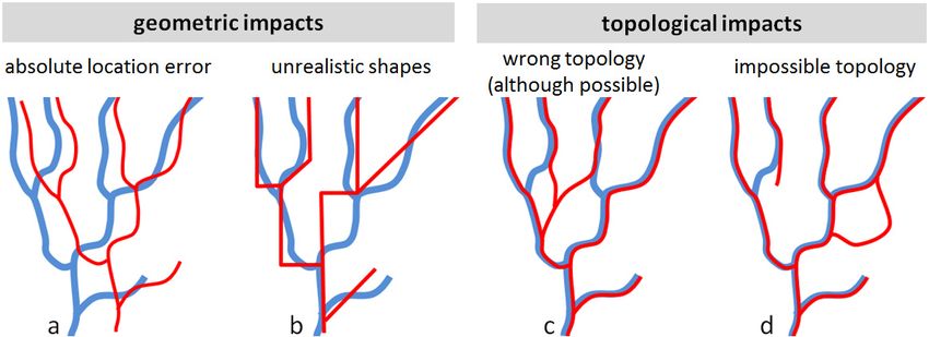
Remote Sens. 2020, 12, x FOR PEER REVIEW 2 of 36
aerial Sens.
Remote photography,
2020, 12, 3522 and it became the standard method for elevation mapping worldwide 2after
of 36
World War II.
(a) (b)
1. Cartographic representation of terrestrial relief in maps in Southern
Figure 1. Southern France:
France: Cassini map,
18th century
18th century (a);
(a); IGN
IGN map,
map, 1957
1957 (b).
(b).
Several
Several major
majorinnovations
innovationstook
tookplace during
place thethe
during lastlast
quarter of the
quarter of20th
the century: black black
20th century: and white
and
photography gave way to color, analytical photogrammetry became the standard
white photography gave way to color, analytical photogrammetry became the standard forfor three-dimensional
(3D) mapping, digital
three-dimensional (3D)databases
mapping,were implemented
digital by mapping
databases were agencies,
implemented and a growing
by mapping variety
agencies, andofa
platforms, sensors, and processing methods extended the possibility of photogrammetry,
growing variety of platforms, sensors, and processing methods extended the possibility of which became
an increasingly powerful
photogrammetry, toolbox an
which became [4]:increasingly powerful toolbox [4]:
•• New
New platforms
platformsextended
extendedthethe capabilities
capabilities of the
of aircraft: satellites
the aircraft: covering
satellites largerlarger
covering areas (first
areasTIROS
(first
observation satellitesatellite
TIROS observation in 1960, across-track
in 1960, across-trackstereoscopy fromfrom
stereoscopy different orbits
different with
orbits SPOT-1
with SPOT-1 in
1986, along-track stereoscopy with SPOT-5 in 2002), UAVs (fixed-wing
in 1986, along-track stereoscopy with SPOT-5 in 2002), UAVs (fixed-wing for large for large area surveys,
multirotor
multirotor for
for small
small area
area surveys
surveys requiring
requiring agility
agility and precision), and mobile mapping systems
on
on land
land vehicles.
vehicles.
•• processing methods
New processing methods were were developed,
developed, such as as aerotriangulation
aerotriangulation and automatic automatic image
image
matching that
matching thatmade
made it possible
it possible to process
to process large quantities
large quantities of images offorimages for theproduction
the industrial industrial
production
of orthophoto ofmosaics
orthophoto mosaics and
and altimetric altimetric
databases withdatabases
few ground with few ground
control control
points [5], points
and the [5],
synergy
and the synergy
between between digital photogrammetry
digital photogrammetry and computer vision and computer
led to very vision led to3D
powerful very powerful 3D
reconstruction
reconstruction
methods such as methods such as from
SfM (structure SfM (structure
motion). from motion).
•• sensors broadened
New sensors broadened the the imaging
imaging possibilities,
possibilities, like spaceborne
spaceborne and airborne SAR (synthetic
aperture radar)
aperture radar)[6–8]
[6–8]andandlidar
lidar[9,10],
[9,10],i.e.,
i.e., active
active sensors
sensors thatthat
mademade it possible
it possible to acquire
to acquire datadata
day
day and night, even in cloudy areas and
and night, even in cloudy areas and beneath forests. beneath forests.
These innovations
These innovationscontributed
contributed torapid
to the the development
rapid development of geographic
of geographic information
information technologies
technologies
by providingby providing
a vast amount a vast amount
of data, amongof data,
whichamong whichelevation
the digital the digitalmodel
elevation
(DEM)model (DEM)
is one is
of the
one of the most widely utilized. Both public and private initiatives have led to an
most widely utilized. Both public and private initiatives have led to an increasing availability of digitalincreasing
availability
elevation of digital
models, eitherelevation
produced models,
on demand either produced
or stored on demand
in multi-user or stored
databases. in stimulated
This has multi-user
databases.
the This has
development of a stimulated
wide rangethe development
of applications in of a wide
which range of description
a quantitative applicationsofinthewhich
terraina
quantitative description of the terrain geometry is needed, such as geoscientific studies
geometry is needed, such as geoscientific studies (flood or landslide hazard assessment) [11,12] and (flood or
landslide hazard assessment) [11,12] and those based on spatial analysis (soil properties,
those based on spatial analysis (soil properties, location of a telecommunication tower or of a new location of
a telecommunication
company) [13,14], etc.,tower
as wellorasofimage
a neworthorectification
company) [13,14], etc., as
[15,16]. wellofasthose
Some image orthorectification
applications require
shape and topology description based on quantitative terrain descriptors extracted fromon
[15,16]. Some of those applications require shape and topology description based quantitative
DEMs, such as
terrainmaps,
slope descriptors
drainageextracted
networks,from DEMs, such
or watershed as slopeleading
delineation, maps, to drainage networks,
the emergence of a or
new watershed
scientific
delineation,
discipline leading
called to the emergence[12,17–19].
“geomorphometry” of a new scientific discipline called “geomorphometry” [12,17–
19]. As with any other product, the ability of a DEM to fulfil user requirements is characterized by a
number of quality criteria. Once the general characteristics of the DEM have been agreed (resolution,
spatial coverage, date etc.), the main requirements relate to the quality of the data themselves, which can
Remote Sens. 2020, 12, 3522 3 of 36
be divided into two main types, namely, elevation quality (generally defined in terms of absolute or
relative accuracy) and shape and topologic quality (related to the accuracy of DEM derivatives such
as slope, aspect, curvature etc. that are quantitative descriptors of the relief [11,20–23]). The quality
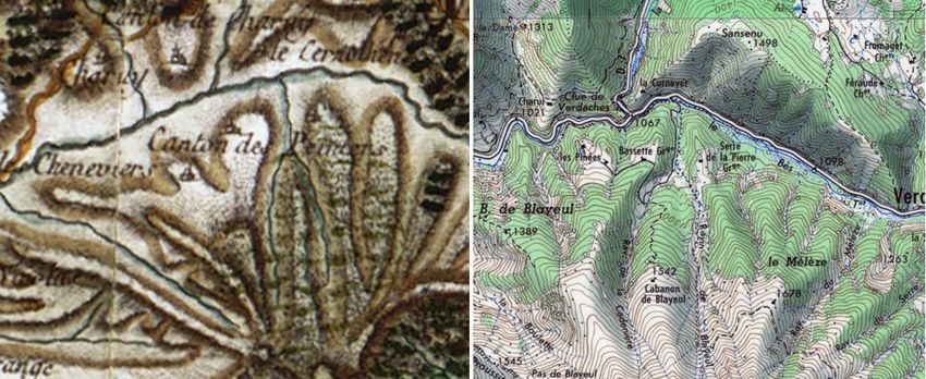
of these descriptors is decisive for the applications that use them [24]. If we express these two types
of quality criteria in natural language, they mean that the model must be as close as possible to
the real terrain position, and that it must look as much as possible like the real terrain, respectively.
These two types of requirements are not equivalent, and it seems relevant to consider both of them.
Indeed, a small position error can induce erroneous shape representations [25–27]. On the other
hand, a high autocorrelation of the elevation error tends to preserve terrain shape quality despite high
positional errors [28].
The terrestrial relief surface has specific characteristics, different from those of most surfaces
represented in geographic information, which make DEM quality assessment a challenging task:
• DEM is multi-user information, so that multiple quality criteria must be met, and although a
particular user may specify application-driven requirements, the case of multi-user databases is
obviously more complex.
• The Earth’s surface is a material object that speaks to our senses, so that one can complain about
unrealistic relief modelling even in an unknown region; this leads to strong requirements including
aesthetic ones.
The aim of this article is to discuss the issue of DEM quality assessment and to propose a review
of the main approaches. Defining the nominal terrain and specifying the characteristics of the digital
product are two prerequisites of DEM quality assessment that are addressed in Sections 2 and 3,
respectively. Section 4 is the core of the article, with a review of relevant quality criteria for DEMs.
This review encompasses a variety of quality assessment methods, based or not on reference data.
Section 5 shows that these criteria can be considered at different levels, i.e., from point cloud to grid
surface model, from grid surface model to topographic features, and at the global level. Section 6 shows
that the resolution of a DEM should also be considered in its quality assessment. Finally, an overall
discussion is proposed in Section 7.
2. Prerequisite: Definition of the Nominal Terrain
Assessing the quality of a DEM requires a clear and explicit definition of the nominal surface,
i.e., the physical surface which is supposed to be modelled. Two nominal surfaces are often considered,
namely the ground surface (represented in a DTM—digital terrain model) and the upper surface above
the trees, buildings and all other natural or manmade objects (represented in a DSM—digital surface
model, provided by most DEM production techniques such as photogrammetry and short wavelength
radar technologies). It should be noted that DEM is a generic term that applies to both cases.
The choice between DTM and DSM depends on the foreseen application. For instance, a DSM
is well suited for orthorectification of imagery as it requires information on the elevation of the top
of buildings and trees, i.e., objects visible in the images, whereas a DTM is required for hydrological
modelling that needs information on the level of the ground where surface water runs off.
As illustrated in Figure 2, the DSM is defined over any area, including in the presence of buildings
(roofs) or trees (canopy). On the other hand, the DTM is defined in bare terrains as well as in forested
areas (the ground surface exists and it controls the surface runoff although the presence of trees
modifies the process), but not in the presence of a building, since in this case the ground surface does
not physically exist (it can be interpolated to generate a continuous surface but this is meaningless for
many applications, like hydrological modelling).
The nuance between DSM and DTM does not exist on other planets, nor on the seafloor, while it
is relevant for the modelling of Earth continental surfaces due the abundance of trees and buildings.
In many landscapes, the reality is even more complex, for example in the presence of grass vegetation
whose height would be comparable to the precision of the topographic method: validating a DEM
Remote Sens. 2020, 12, 3522                                                                         4 of 36

obtained by photogrammetry or even lidar, where the measured elevation lies at the top of the grass,
by comparison with control points measured on the ground, can lead to an erroneous conclusion on the
accuracy of the DEM and therefore of the mapping method, since the reference data do not represent
the same surface as the DEM. Consequently, it would be meaningless to evaluate the quality of a DEM
 Remote Sens.
without       2020, definition
          a clear   12, x FOR PEER  REVIEW
                                of the physical surface it is supposed to represent.             4 of 36

                              Figure 2. DTM vs DSM in the presence of trees and buildings.
                               Figure 2. DTM vs DSM in the presence of trees and buildings.
       Given the variety of relief mapping techniques, which are sensitive to different aspects of the
        The nuance between DSM and DTM does not exist on other planets, nor on the seafloor, while it
terrain surface, it is highly recommended that the most appropriate technique be chosen according
 is relevant for the modelling of Earth continental surfaces due the abundance of trees and buildings.
to the selected nominal terrain. In the presence of forests, photogrammetry and short wavelength
 In many landscapes, the reality is even more complex, for example in the presence of grass
radar techniques are more appropriate for DSM than for DTM, while lidar and long wavelength radar
 vegetation whose height would be comparable to the precision of the topographic method:
techniques are suitable for both surface models [29,30]. However, it is not always possible to access
 validating a DEM obtained by photogrammetry or even lidar, where the measured elevation lies at
the ideal technique. For example, it is very common to use photogrammetry to produce a DTM
 the top of the grass, by comparison with control points measured on the ground, can lead to an
(i.e., the nominal terrain is the ground surface). In order to prevent users from making gross errors by
 erroneous conclusion on the accuracy of the DEM and therefore of the mapping method, since the
using such information in forested areas, postprocessing strategies must be employed to remove tree
 reference data do not represent the same surface as the DEM. Consequently, it would be
height so that the DEM can theoretically be considered as a DTM.
 meaningless to evaluate the quality of a DEM without a clear definition of the physical surface it is
       In the case of sand or ice deserts, two possible nominal surfaces can be considered, namely,
 supposed to represent.
the bedrock and the upper sand or ice surface which is in contact with the atmosphere. It is relevant to
        Given the variety of relief mapping techniques, which are sensitive to different aspects of the
define which of these surfaces is supposed to be represented in a DEM since the expectations will be
 terrain surface, it is highly recommended that the most appropriate technique be chosen according
different. Indeed, the bedrock is stable over time and its shape is most often generated by tectonics and
 to the selected nominal terrain. In the presence of forests, photogrammetry and short wavelength
long-term hydric erosion, while the shape of the upper sand or ice surface is constantly changing due
 radar techniques are more appropriate for DSM than for DTM, while lidar and long wavelength
to climatic processes and gravity. No operational technique, except field survey, is currently available
 radar techniques are suitable for both surface models [29,30]. However, it is not always possible to
to map the substratum in such areas for the Earth, but the future Biomass mission could bring new
 access the ideal technique. For example, it is very common to use photogrammetry to produce a
opportunities thanks to the penetrating capabilities of its P-band radar [31].
 DTM (i.e., the nominal terrain is the ground surface). In order to prevent users from making gross
       The case of shallow water bathymetry (i.e., rivers or coastal sea water) raises the question of
 errors by using such information in forested areas, postprocessing strategies must be employed to
the nominal terrain as well. Indeed, the surface and the bottom of the water have different physical
 remove tree height so that the DEM can theoretically be considered as a DTM.
behaviours with regards to existing imaging sensors and the image of this double surface must be
        In the case of sand or ice deserts, two possible nominal surfaces can be considered, namely, the
interpreted with caution. For example, photogrammetry and green lidar can survey the bottom
 bedrock and the upper sand or ice surface which is in contact with the atmosphere. It is relevant to
topography in the case of clear water [32,33] but the signal is attenuated by the presence of the water,
 define which of these surfaces is supposed to be represented in a DEM since the expectations will be
whereas radar imagery only surveys the surface but the image is influenced by the bottom topography.
 different. Indeed, the bedrock is stable over time and its shape is most often generated by tectonics
At low tide, only the ground appears and it can be reconstructed in 3D [34,35].
 and long-term hydric erosion, while the shape of the upper sand or ice surface is constantly
       The nominal terrain considered in a DEM, which is supposed to be defined in agreement with
 changing due to climatic processes and gravity. No operational technique, except field survey, is
the user’s requirements, should be clearly indicated for users’ information. Nevertheless, important
 currently available to map the substratum in such areas for the Earth, but the future Biomass mission
altimetric products such as SRTM and TanDEM-X global DEMs do not clearly specify the nominal
 could bring new opportunities thanks to the penetrating capabilities of its P-band radar [31].
terrain. Although X- and C-band SAR interferometry rather provides a DSM and no filtering is applied
        The case of shallow water bathymetry (i.e., rivers or coastal sea water) raises the question of the
to the native products to transform them into DTMs, all information about these products suggests that
 nominal terrain as well. Indeed, the surface and the bottom of the water have different physical
they are specified as ground surface models, and many users regard them as such [36–38]. Considering
 behaviours with regards to existing imaging sensors and the image of this double surface must be
that the nominal surface is the ground implies that elevation discrepancies due to tree height must be
 interpreted with caution. For example, photogrammetry and green lidar can survey the bottom
 topography in the case of clear water [32,33] but the signal is attenuated by the presence of the water,
 whereas radar imagery only surveys the surface but the image is influenced by the bottom
 topography. At low tide, only the ground appears and it can be reconstructed in 3D [34,35].
        The nominal terrain considered in a DEM, which is supposed to be defined in agreement with
 the user’s requirements, should be clearly indicated for users’ information. Nevertheless, important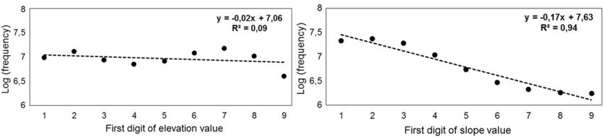
Remote Sens. 2020, 12, 3522                                                                            5 of 36

interpreted in terms of DEM error. In other words, they contribute to the fact that the DEM does not
fulfil user requirements for geoscientific studies.
      The need for a clear specification of the nominal terrain in the metadata has become even more
critical with the growing development of high resolution and high precision products, which have
stimulated applications based on the modelling of small objects, such as buildings or parts of buildings,
in synergy with topographic methods like terrestrial or mobile laser scanning of urban scenes. In the
case of buildings that are very complex objects, the need for simplification has led to the definition
of level of detail (LOD) standards that can help to specify user requirements [39,40]. Moreover,
undesirable objects such as vehicles or street furniture may appear in the input data and the need
to include them depends on the DEM application. Similarly, when a bridge spans a road or a river,
the product specification must clearly indicate whether the bridge is modeled (which could lead to
large errors in hydrological modeling) or not (which could generate artifacts in the orthophotos created
using the DEM).

3. DEM as a Cartographic Product
     The altimetric information collected to represent the terrain surface is generally represented in
the form a cartographic product, which is defined by a number of specifications. Traditional paper
maps are specified with a scale, a cartographic projection and a legend that indicates how the map
describes the terrain. Similarly, the DEM is characterized by metadata, i.e., data about the DEM itself,
which make possible the access to the altimetric data in the digital file and provide information such
as the producer, the date, the accuracy etc. In this section, we show that the Earth’s surface has very
special properties (Section 3.1) which influence the way a DEM must be specified, i.e., the structure of
the planimetric grid (Section 3.2) and the numerical representation of the elevation (Section 3.3).

3.1. A Very Peculiar Surface
     Unlike most physical surfaces represented by 3D models for robotics, architecture, industry etc.,
the Earth’s relief has a very particular property: it can be considered as a 2.5D surface. Indeed, once the
nominal terrain has been defined (e.g., the ground surface), a unique altitude z can be assigned to each
horizontal position (x, y). This is due to the gigantic mass of the Earth (M ~6.1024 kg) and the intensity
of the associated gravitational field (g ~9.8 m·s−2 ), where the attraction of all material particles towards
the mass center gives the Earth’s spherical shape. As a result, the Earth’s surface has almost no hidden
part when seen from above. It is comparable to a bas-relief which has no hidden part when seen from
the front. This property is not cancelled out by the centrifugal force produced by the Earth’s rotation,
which transforms the sphere into an ellipsoid.
     A few exceptions exist, like overhang cliffs where more than one elevation value can be assigned
to a given horizontal position. But they are rare enough to justify the general assumption that any
vertical axis (from the Earth’s center to the zenith) has a unique intersection with the topographic
surface (Figure 3). This is the definition of a 2.5D surface and it has a very interesting advantage since
the elevation can be considered as a bivariate function z = f(x, y). Indeed, most cartographic systems
consist in separating two planimetric coordinates (latitude and longitude or equivalent) on the one
hand, and a vertical coordinate (altitude above sea level) on the other hand. Therefore, the specification
of a DEM as a cartographic product consists in specifying two aspects: the planimetric grid structure
and the numerical representation of elevation values, beyond the classical specifications of all maps
like datum and map projection. These specification data are essential. They are generally available as
metadata with the DEM file. Our aim is not to recall this well-known information in detail, since it has
been widely addressed in GIS literature [41], but to stress the need for an explicit specification as a
condition for DEM quality assessment.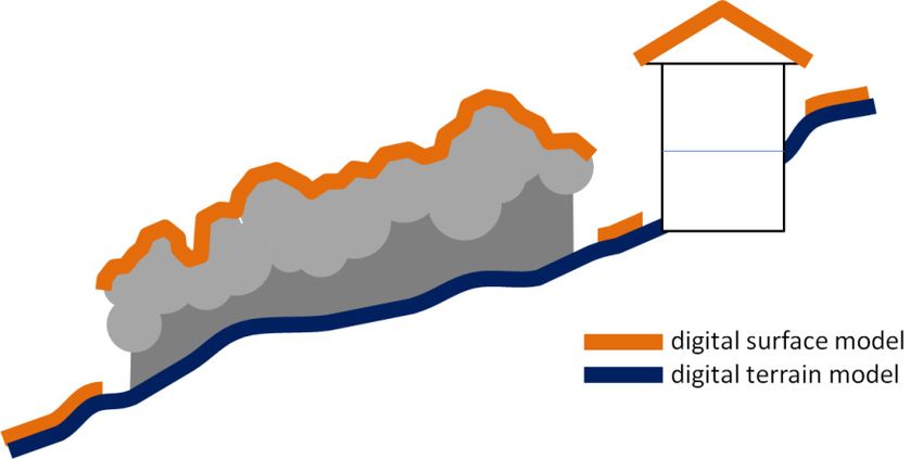
x FOR PEER REVIEW
Remote Sens. 2020, 12, 3522                                                                             6 of 36

            Figure 3. 2.5D representation of the Earth’s surface: general case (a) and exception (b).

3.2. Planimetric Grid Sructure
3.2. Planimetric Grid Sructure
      Most relief mapping techniques consist of two steps, namely, altitude computation for a large
      Most relief mapping techniques consist of two steps, namely, altitude computation for a large
number of terrain points, and resampling to fit the specifications of the output product when necessary.
number of terrain points, and resampling to fit the specifications of the output product when
The technique implemented to compute terrain altitudes with specific acquisition and processing
necessary. The technique implemented to compute terrain altitudes with specific acquisition and
parameters has an impact on the positional accuracy of each point and on the density of the resulting
processing parameters has an impact on the positional accuracy of each point and on the density of
point cloud. However, the DEM quality is not limited to these aspects since the subsequent resampling
the resulting point cloud. However, the DEM quality is not limited to these aspects since the
step could also have a major impact on the quality of the output DEM. Two important specifications
subsequent resampling step could also have a major impact on the quality of the output DEM. Two
are set up to define the resampling procedure, i.e., the grid structure and the interpolation algorithm.
important specifications are set up to define the resampling procedure, i.e., the grid structure and
the interpolation
3.2.1.             algorithm.
       Grid Structure

3.2.1.The
       Gridgrid structure defines the planimetric positions in which the altimetric values are to be stored.
             Structure
Two main grid structures may be considered, namely, regular (e.g., a square mesh raster grid) and
      The grid structure defines the planimetric positions in which the altimetric values are to be
irregular structures (e.g., a triangular irregular network).
stored. Two main grid structures may be considered, namely, regular (e.g., a square mesh raster
      The regular grid has clear advantages in terms of data handling. Indeed, the horizontal coordinates
grid) and irregular structures (e.g., a triangular irregular network).
are implicit, and they theoretically do not need to be stored provided that they are logically defined by
      The regular grid has clear advantages in terms of data handling. Indeed, the horizontal
metadata, and the square mesh grid can be displayed directly on a screen or a printout with no need
coordinates are implicit, and they theoretically do not need to be stored provided that they are
for further resampling. The regular grid structure is defined a priori (i.e., regardless of the distribution
logically defined by metadata, and the square mesh grid can be displayed directly on a screen or a
of the input point cloud), but most data acquisition methods provide irregularly distributed points so
printout with no need for further resampling. The regular grid structure is defined a priori (i.e.,
that an interpolation step is required to resample the data in order to fit the regular grid. Conversely,
regardless of the distribution of the input point cloud), but most data acquisition methods provide
no resampling is required for the irregular structure, which is built a posteriori over previously acquired
irregularly distributed points so that an interpolation step is required to resample the data in order
points. It is typically the case of the well-known TIN (triangular irregular network): this structure
to fit the regular grid. Conversely, no resampling is required for the irregular structure, which is
consists of a network of non-overlapping planar triangles built on the preliminary point cloud [42,43].
built a posteriori over previously acquired points. It is typically the case of the well-known TIN
Intermediate grid structures have been proposed, like for progressive or composite sampling [44,45],
(triangular irregular network): this structure consists of a network of non-overlapping planar
in which a regular grid is iteratively densified as long as the curvature exceeds a given threshold,
triangles built on the preliminary point cloud [42,43]. Intermediate grid structures have been
leading to a semi-regular grid of variable density [46–48]. This multiresolution modeling approach has
proposed, like for progressive or composite sampling [44,45], in which a regular grid is iteratively
gained interest for interactive terrain visualization [49].
densified as long as the curvature exceeds a given threshold, leading to a semi-regular grid of
      The size and shape of the grid mesh must be specified with care due to their impact on the
variable density [46–48]. This multiresolution modeling approach has gained interest for interactive
DEM quality.
terrain visualization [49].
•     The size
           mesh   size
                and    (andoftherefore
                     shape               the grid
                               the grid mesh   mustdensity) has anwith
                                                     be specified   impact
                                                                       care on
                                                                            duethe DEMimpact
                                                                                to their absolute
                                                                                               on accuracy,
                                                                                                   the DEM
      but also on the ability of the DEM to describe landforms as shown below in Section 4.2. This ability
quality.
      is intuitive, since a smaller mesh is expected to allow a better rendering of small topographic
• The mesh size (and therefore the grid density) has an impact on the DEM absolute accuracy, but
      objects, but a signal processing approach may also provide criteria to optimize resampling and to
     also on the ability of the DEM to describe landforms as shown below in Section 4.2. This ability is
      detect DEM errors [50]. The link between mesh size and resolution, and the way DEM quality
     intuitive, since a smaller mesh is expected to allow a better rendering of small topographic
      assessment should consider these concepts, are addressed in Section 6.
     objects, but a signal processing approach may also provide criteria to optimize resampling and
•     The mesh shape has an influence on the adequacy of the surface modelling to local landforms.
     to detect DEM errors [50]. The link between mesh size and resolution, and the way DEM quality
      Between the two most common grid structures, namely constant size squares and variable size
     assessment should consider these concepts, are addressed in Section 6.
      triangles, the latter is clearly better suited to describe a surface morphology in which drainages,
• The mesh shape has an influence on the adequacy of the surface modelling to local landforms.
      ridges and other slope breaks have variable orientations. However, there are several solutions to
     Between the two most common grid structures, namely constant size squares and variable size
      build a network of triangles from a given point cloud. For example, the Delaunay triangulation
     triangles, the latter is clearly better suited to describe a surface morphology in which drainages,
      is advantageous to avoid very elongated triangles (which are less suitable for spatial analysis),
     ridges and other slope breaks have variable orientations. However, there are several solutions to
Remote Sens. 2020, 12, 3522                                                                            7 of 36

      but it does not necessarily give the most accurate DEM nor the most respectful one of terrain
      shapes: it must therefore be constrained so that the edges of the triangles are placed along slope
      discontinuities such as drainages or other slope break lines. This is an advantage of triangle
      networks, which are able to adapt to the topography.

3.2.2. Interpolation Algorithm
     Between the grid points, the surface model is built by interpolation so that the elevation and
its derivatives can be determined at any planimetric position. The interpolation is based on the
input points on the one hand, and on a generic mathematical surface model on the other hand.
There are different interpolation algorithms and they can affect the quality of the resulting DEM [51].
The interpolator has less influence on the quality of the DEM if the initial point cloud is dense or if
the grid is irregular with selected points on the slope breaks. Indeed, in these cases the mesh of the
surface model remains close to the ground and a smooth interpolator can be used. On the other hand,
the interpolator has a great influence on the quality of the DEM if the grid points have a low density,
or in the presence of holes (missing information) which can occur as a result of the presence of a cloud
in photogrammetry or a forest in repeat-pass SAR interferometry.
     A great variety of interpolators are used in geoscience for interpolating thematic data to produce
raster maps [52], but they are not always relevant for DEMs, since the performances achieved for
moisture or geochemical concentrations, for instance, have no reason to be effective for elevation.
Some algorithms generate altimetric variability, like kriging or fractal zoom. These two different
mathematical formalisms aim at calculating and analyzing the variability around the interpolated
mesh and propagating it at a finer scale within the mesh [53]. It is a way to guarantee geomorphologic
realism as compared to usual interpolators [54].

3.3. Numerical Representation of Elevation Values
     Elevation values are generally defined as altitudes, i.e., measured relative to a horizontal surface
that models the Earth at sea level. It is a gravimetric definition of elevation, suitable for many
applications based on hydrologic or hydraulic modelling. With the space age, a global reference
was sought, such as a global geoid model, and the fact of locating points by satellite (e.g., GNSS)
led to prefer a geometric definition of the reference surface, typically an ellipsoid such as WGS84
(World Geodetic System), easier to handle than a geoid model. The coexistence of geometric and
gravimetric references requires conversions between systems, and it is a source of confusion [55–57].
     Even if some software tools assign elevation values to surface elements (i.e., pixels), this information
is only relevant when assigned to a Euclidean point, defined by its coordinates which are easy to
store and used to compute distances, angles and other metrics. However, except high precision
topometric techniques (e.g., total station and GNSS), all techniques compute a mean elevation over a
local neighborhood. In a DEM generated by digital photogrammetry for example, the image matching
process is based on the correlation between small windows of a given size, typically several pixels,
and the resulting elevation, though assigned to a point position (x, y), is influenced by the elevation
distribution over a terrain area [58].
     The bit depth is also an important product specification for a DEM, since it has an impact on
the data volume and on the vertical quantization. Early generation DEMs were generally coded on
8 bits because they were not very precise and computers had limited storage capacities. It was a
limitation, mainly in plain areas where step-like artifacts could appear on the ground surface. Since the
1990s, the floating-point representation has been enabled by 16 or 32-bit encoding to represent decimal
numbers, increasing the precision and the elevation range for DEM storage. A 16-bit depth is good
enough for global DEMs such as SRTM, with a 5–10 m range of accuracy and a 1-m quantization
unit [59–61]. However, a 32-bit depth is preferable for high accuracy DEM as obtained by aerial or
terrestrial photogrammetry or by laser scanning.
     All these specifications are essential to guarantee the quality of a digital elevation model.
Remote Sens. 2020, 12, 3522 8 of 36
Remote Sens. 2020, 12, x FOR PEER REVIEW 8 of 36
4.4.Main
MainDEM
DEMQuality
QualityAssessment
AssessmentApproaches
Approaches
The validation
The validationof of aa DEM
DEM consists
consists inin assessing
assessing its
its ability
ability to
to fulfil
fulfil user
user requirements
requirements based
based onon
adapted quality criteria. For each criterion, a quality assessment procedure can
adapted quality criteria. For each criterion, a quality assessment procedure can be implemented to be implemented to
decidewhether
decide whetheraaDEMDEMisisacceptable
acceptablefor
foraagiven
givenuseuse[62].
[62].In Inthis
thissection,
section,we wereview
reviewthe
themain
mainquality
quality
assessment approaches. Although this review is not exhaustive, it illustrates the variety
assessment approaches. Although this review is not exhaustive, it illustrates the variety of existing of existing
methodscommonly
methods commonlyused usedby byproducers
producers andand users.
users. We
Weshowshowthat
thatDEM DEM quality
quality assessment
assessmentcan
can be
be
consideredwith
considered withoror without
without ground
ground reference
reference data.
data. InInthe
thefirst
firstcase,
case,the theDEM
DEMisiscompared
comparedwith
withaa
reference data set (external validation), whereas in the second case, inconsistencies are
reference data set (external validation), whereas in the second case, inconsistencies are sought within sought within
theDEM
the DEMitself
itselfwith
withnonoreference
reference data
data (internal
(internal validation).
validation).
4.1. External Quality Assessment
4.1. External Quality Assessment
4.1.1. Comparison with Ground Control Data
4.1.1. Comparison with Ground Control Data
The goal of the external validation is to assess the quality of a DEM using external reference data,
whichThe goal
can be aofsparse
the external
cloud of validation is to assess
points, contour lines,the quality ofprofiles,
topographic a DEM using external
or a much morereference
accurate
data, which can be a sparse cloud of points, contour lines, topographic profiles,
DEM. A comprehensive overview of external validation methods can be found in [63]. As mentioned or a much more
accurate DEM. A comprehensive overview of external validation methods can be
in Section 3, a DEM is a digital 2.5D representation of the Earth’s surface, in which the elevation found in [63]. As
mentioned in Section 3, a DEM is a digital 2.5D representation of the Earth’s surface,
is a bivariate function z = f(x, y). Thus, the quality of a DEM includes planimetric and altimetric in which the
elevation
components. is a Most
bivariate function
of the studieszaim= f(x, y). Thus, the
at evaluating thequality
verticalofquality
a DEM in includes planimetric
a DEM, i.e., and
the altimetric
altimetric components. Most of the studies aim at evaluating the vertical quality in
quality rather than the planimetric quality. The usual approach consists in computing some statistical a DEM, i.e., the
altimetric quality rather than the planimetric quality. The usual approach consists
indicators based on the altimetric discrepancies between the DEM and the reference. As a rule of in computing
some
thumb, statistical indicators
the reference based
dataset mustonfulfil
the altimetric
two maindiscrepancies
requirements:between the DEM and the reference.
As a rule of thumb, the reference dataset must fulfil two main requirements:
• It must be much more accurate than the evaluated DEM.
• It must be much more accurate than the evaluated DEM.
• It must be dense enough and well distributed over the area to allow meaningful statistical analysis,
• It must be dense enough and well distributed over the area to allow meaningful statistical
and even a spatial analysis of the error.
analysis, and even a spatial analysis of the error.
The altimetric error of a DEM is composed of three main components, namely, gross, systematic
and The altimetric
random errorserror of aasDEM
[64,65] shown is composed
in Figure of4. three main components,
A systematic namely,
error is a bias betweengross,
thesystematic
modelled
and random
surface and theerrors [64,65]
ground truthasand
shown in Figure
it depends 4. A
on the systematic
production error is aespecially
technique, bias between the acquisition
the data modelled
surface and thebut
configuration, ground
also ontruth and it depends
the interpolation methodon [66].
the production technique,
It can be calculated usingespecially the value
the average data
acquisition configuration, but also on the interpolation method [66]. It can
of the elevation difference between the DEM and the reference data. Random errors are mainly duebe calculated using the
to
average value of the elevation difference between the DEM and the reference data.
the production technique and they are mostly influenced by the quality of the raw data, the processing Random errors
are mainly due
parameters, to the
as well asproduction technique and
the terrain morphology andthey
theare mostly influenced
vegetation by the
[67]. They are qualitythrough
evaluated of the raw
the
data,
calculation of the standard deviation of the elevation difference. Gross errors are outliers They
the processing parameters, as well as the terrain morphology and the vegetation [67]. are
resulting
evaluated
from faultsthrough
during the
the calculation
productionof ofthe
the standard
DEM. deviation of the elevation difference. Gross errors
are outliers resulting from faults during the production of the DEM.
Figure 4. Main behaviours of DEM error.
Figure 4. Main behaviours of DEM error.
As any other geographic data, the elevation in a DEM has a spatial behaviour and so does its
AsIndeed,
error. any other geographic
although a partdata, theelevation
of the elevationerror
in a is
DEM has a itspatial
random, behaviour
is often spatiallyand so does its
autocorrelated,
error. Indeed, although a part of the elevation error is random, it is often spatially autocorrelated,
which means that neighboring points tend to have comparable errors [68,69]. Thus, the random error
which means that neighboring points tend to have comparable errors [68,69]. Thus, the random error
is a combination of two types of random variables: one is spatially autocorrelated whereas the otherRemote Sens. 2020, 12, 3522 9 of 36
is a combination of two types of random variables: one is spatially autocorrelated whereas the other is
a pure noise [70]. This autocorrelation can also be anisotropic [71]. Then, the elevation of a particular
point in a DEM is the sum of its true elevation and the aforementioned errors:
ẑi = zi + µ + ε0 i + ε00 i (1)
where ẑi is the altitude in the DEM, zi is the true altitude on the terrain, µ is the systematic error (bias),
ε0 i is the spatially autocorrelated random error, and ε00 i is the spatially non-autocorrelated random
error (pure noise).
External quality assessment consists in analyzing the whole set of elevation discrepancies
(µ + ε0 i + ε00 i ), calculated between the DEM and a set of ground control points (GCPs), based on
simple statistical indicators such as the mean, the standard deviation, the root mean square error
(RMSE), the maximum error etc. [69]. These indicators are used to assess the DEM error in terms
of altimetric accuracy and precision [67]. Note that the terms related to data uncertainty are often
used in a confusing way [72]. The third edition of the Photogrammetric Terminology [73] defines
accuracy as “the closeness of the result of a measurement, calculation or process to the true, intended
or standard value”, and precision as “the repeatability of a result, including the number of significant
figures quoted, regardless of its correctness” (further clarification on the meaning of these words and
on the pitfalls of translation can be found in [74]).
The most commonly used statistical indicator is the RMSE [65], which provides a reliable indication
on the altimetric DEM error considering that the sample size N of the reference data (i.e., the number
of GCPs) is big enough [43]:
s
Pn 2
i=1 (ẑi − ziRef )
RMSE = (2)
N
The relationship between the RMSE, the mean, and the standard deviation of the error is
the following:
p
RMSE = µ2 + σ2 (3)
The statistical distribution of the error is often Gaussian [28], although some studies suggest
that this hypothesis is not always valid [75]. To verify the validity of this hypothesis, Q-Q plots
(quantile-quantile plots [63,75]) can be used. This can be helpful to reveal a non-normal distribution
and to suggest more adapted statistical indicators for error analysis, like the median, which is more
robust, i.e., not affected by extreme error values. If we consider that the error follows a normal
distribution N(µ,σ), then it is possible to define the confidence level of the error that corresponds to
the percentage of points whose error value lies in the confidence interval. For instance, the intervals
[µ − σ; µ + σ] and [µ − 1.96σ; µ + 1.96σ] correspond to linear errors with 68% (LE68) and 95% (LE95)
confidence levels, respectively.
The elevation error propagates through elevation derivatives like slope, aspect and curvature,
leading to erroneous drainage network or watershed delineation for instance [76,77]. Although the
computation of the slope or other derivatives may lead to different results according to the selected
algorithms [78–82], the error propagation always generates an uncertainty in the resulting product
(e.g., slope map) that needs to be evaluated due to its wide use in many applications of DEMs
in geoscience [68,82–84]. In general, the elevation derivatives are very sensitive to the spatial
autocorrelation of the error [28]. Indeed, since the elevation derivatives are calculated using a
neighborhood, their quality depends on the error of the points from which they have been extracted
as well as on the autocorrelation of their errors. Then, it is possible to have a low positional quality
but a high quality of the derivatives as in the case of a big systematic error and a small random error,
and vice versa.
Most DEMs are delivered with a simple value of the RMSE or a standard deviation of the elevation
error, and this value is considered as representative of the overall quality of the DEM, where the spatialor mountainous areas. Thus, to assess the error propagation from the elevation to its derivatives, an
error model has to be built (Figure 5).
This error model includes the elevation error as well as its autocorrelation and it can be
modelled using a semivariogram. The following formula represents an exponential error model [85]:
Remote Sens. 2020, 12, 3522 10 of(4)
36
γ(h) = σ (1 − e )
where γ is the semivariance, h is the horizontal distance, σ is the sill and φ is the range. An error
distribution
model having of the errornugget
a null is completely ignored [71].
(i.e., y-intercept), This is due
a minimal silltoand
the fact that the evaluation
a maximum practical of the
range
spatial autocorrelation of the error requires a dense sample of control points,
provides a high spatial autocorrelation and then a high quality of elevation derivatives. The which in many cases is
not available.
generation of However,
the modelalthough
is basedthe on RMSE is well adapted
the second-order for the hypothesis,
stationary positional quality
whichassessment of a
supposes that
DEM, it may not be informative about the quality of elevation derivatives
the mean and the standard deviation of the error are constant in the DEM and that the since it does not consider
the spatial behaviour
autocorrelation of theof error
the error [27]. This[69].
is isotropic behaviour can reveal
The isotropic systematicwhich
hypothesis, trendsisduenottonecessarily
inaccurate
orbit or sensor
verified model parameters
in the natural relief due toastectonic
well asorlocal error autocorrelation,
hydrographic phenomena, often
mayduealsotobethe influence by
questioned of
landscape characteristics, e.g., higher error in forested or mountainous areas. Thus,
the DEM production process, i.e., the data acquisition geometry (as in the case of side looking radar),to assess the error
propagation
the processing from the elevation
method to its derivatives,
(image matching an error
along lines) or themodel has to be (raster
grid structure built (Figure
effect)5).
[86].
Figure 5. Method for the elaboration of an elevation error model.
Figure 5. Method for the elaboration of an elevation error model.
This error model includes the elevation error as well as its autocorrelation and it can be modelled
The error propagation
using a semivariogram. can be measured
The following either analytically
formula represents an exponential whenerror
possible
modelor[85]:
numerically
through simulation-based (e.g., Monte Carlo) methods when it is not analytically possible [68]. The
2 h
−on
goal is to evaluate the impact of data uncertainty
γ(h) = σz 1 − e ϕ the subsequent extracted derivatives (4)
[77,85,87,88]. For instance, the analytically measured error propagation in slope (as it is the most
important
where morphological
γ is the index
semivariance, [89])
h is the calculated
horizontal by trigonometry
distance, σ2 is the sillisand
the ϕ
following [90]:An error model
is the range.
z
having a null nugget (i.e., y-intercept), a minimalz −sillz and a maximum practical range provides a high
S= (5)
d
spatial autocorrelation and then a high quality of elevation derivatives. The generation of the model
is based on the second-order stationary hypothesis,
σ which supposes that the mean and the standard
σ =
deviation of the error are constant in the DEM 2(1that
and − rthe )autocorrelation of the error is isotropic [69].
(6)
d
The isotropic hypothesis, which is not necessarily verified in the natural relief due to tectonic or
where S is the slope, d is the horizontal distance separating points 1 and 2, σ is the error of the
hydrographic phenomena, may also be questioned by the DEM production process, i.e., the data
slope and r is the autocorrelation coefficient of the error. Moreover, in the case of finite
acquisition geometry (as in the case of side looking radar), the processing method (image matching
differences, which give a more accurate slope estimation [91], the slope error for a third-order finite
along lines) or the grid structure (raster effect) [86].
The error propagation can be measured either analytically when possible or numerically through
simulation-based (e.g., Monte Carlo) methods when it is not analytically possible [68]. The goal
is to evaluate the impact of data uncertainty on the subsequent extracted derivatives [77,85,87,88].
For instance, the analytically measured error propagation in slope (as it is the most important
morphological index [89]) calculated by trigonometry is the following [90]:
z2 − z1
S= (5)
d
σz
q
σS = 2(1 − rz1 z2 ) (6)
dRemote Sens. 2020, 12, 3522 11 of 36
where S is the slope, d is the horizontal distance separating points 1 and 2, σS is the error of the slope and
rz1 z2 is the autocorrelation coefficient of the error. Moreover, in the case of finite differences, which give
a more accurate slope estimation [91], the slope error for a third-order finite difference weighted by
reciprocal of squared distance method [79,92–94] is obtained by the following formula [85]:
√ √
3σ2z + 4C(w) − 2C(2w) − 4C 5w − C 8w
σ2S = (7)
16w2
h
C(h) = σ2z − γ(h) = σ2z .e− ϕ (8)
where w is the mesh size and C is the spatial autocovariance.
In a numerical approach, a multiple realization of DEMs is produced based on the error model,
where the precise realization is considered to be one of them. For each realization, the targeted
derivative is extracted, which provides a sample for this derivative. Then, a probabilistic method is
used to evaluate the quality of this derivative [25,85].
All the aforementioned descriptors aim at evaluating the absolute vertical quality and the
derivative quality. In the horizontal dimension, a planimetric shift in the input point cloud has an
impact on DEM elevations that behaves as a planimetric error, which can also be evaluated in both
absolute and relative terms. The absolute planimetric quality is obtained by comparing the planimetric
positions to reference data and adapted statistical descriptors are used to quantify the error like for the
altimetric error as shown above. The relative positional quality is measured between points identified
in the DEM. For instance, the Euclidian distance between two points is obtained using the coordinates
of these points; if we consider these two points have the same error, then the measured distance is not
affected by this error, as in the case of a constant planimetric shift of the DEM.
4.1.2. Simulation-Based DEM Production Method Validation
An interesting extension of external validation consists in processing simulated images to derive
a DEM and to compare the output DEM with the input DEM used to simulate the synthetic image
dataset. In this case, the goal is not to evaluate a particular DEM, but a topographic method used for
DEM production.
This approach implies that computational tools must be available to simulate realistic images
based on a landscape model and a sensor model. Such tools are developed to study radiative transfer
processes and to test remote sensing strategies [95,96]. The landscape model includes its geometry
(DEM and objects over the ground: trees, buildings etc.) and all the characteristics that are relevant to
compute the electromagnetic signal received by the sensor over this particular landscape. The sensor
model includes the description of the sensor itself (spectral interval and any technical property needed
to define the geometry of the images and to compute pixel radiometric values) as well as the acquisition
geometry through the platform position and orientation typically.
Figure 6 shows the workflow that can be implemented for simulation-based validation. Comparing
the input and output DEMs allows the estimation of the error produced by the topographic restitution
method as well as its spatial behaviour. It can also help to better understand the effects of error
propagation. This approach has long been implemented to evaluate the expected performances of
image acquisition strategies as well as processing algorithms for different mapping methods based on
remote sensing data, i.e., photogrammetry [97], lidar [98], and radar methods [99,100]. More recently it
has also been applied to terrestrial mobile mapping [101].Remote Sens. 2020, 12, 3522 12 of 36
Remote Sens. 2020, 12, x FOR PEER REVIEW 12 of 36
Figure 6. General workflow of simulation-based evaluation of topographic restitution methods.
Figure 6. General workflow of simulation-based evaluation of topographic restitution methods.
Although this approach may suffer from a lack of realism that could create biases in the analysis,
Although this approach may suffer from a lack of realism that could create biases in the
it has several advantages such as the possibility to vary the experimental conditions:
analysis, it has several advantages such as the possibility to vary the experimental conditions:
• The topographic restitution method can be tested over a variety of landscapes, leading to more
• The topographic restitution method can be tested over a variety of landscapes, leading to more
comprehensive conclusions than over a particular DEM.
comprehensive conclusions than over a particular DEM.
•
• ItIt can
can also
also be
be tested
tested with
with aa variety
variety of
of sensor
sensor parameters
parameters and
and orbit
orbit configurations,
configurations, leading
leading to
to
recommendations for optimum image acquisition conditions if the images are to be processed
recommendations for optimum image acquisition conditions if the images are to be processed for
DEM
for DEMproduction.
production.
Regarding the lack
Regarding the lack of
of realism,
realism, Figure
Figure 66 suggests some refinements
suggests some refinements to
to overcome
overcome this
this limitation,
limitation,
for instance:
for instance:
•
• The
Theinput
inputDEM
DEMcancan be
bereprocessed,
reprocessed, either
either to to exaggerate
exaggerate the elevation amplitude, or to introduce
topographic
topographic details such
suchas asmicrorelief
microrelieforor buildings
buildings (note
(note thatthat all these
all these changes
changes in theininput
the input
DEM
DEM
can becan be parametrically
parametrically controlled,controlled, allowing analytical
allowing analytical sensitivityFractal
sensitivity studies). studies). Fractal
resampling
resampling can be toimplemented
can be implemented produce a more to realistic
produce a more
input realistic
DEM [102], input DEM [102],
and geomorphology and
provides
geomorphology provides
criteria to verify this realismcriteria to verify
requirement this realism
in accordance requirement
with in accordance
the principles with the
of internal validation
principles
which we of internal
will validation
see further [103]. which we will see further [103].
•
• Sensor
Sensorparameter
parameteruncertainties
uncertaintiescancan be
be introduced
introduced to to consider
consider the
the fact that the DEM production
method
methodalways
alwaysuses
usesanan approximation
approximation of of the
the exact
exact parameters.
parameters.
Since aa dense
Since dense reference
reference dataset
dataset is
is available,
available, the
the principles
principles of
of external
external quality
quality assessment
assessment can
can be
be
fully applied. However, DEM series based on simulated images can also be evaluated
fully applied. However, DEM series based on simulated images can also be evaluated with an internalwith an
internalassessment
quality quality assessment approach,
approach, i.e., with i.e., with no reference
no reference data. data.
4.2. Internal Quality Assessment
Internal quality assessment is implemented with no ground control. It makes use of criteria of
realism based
based on
on aapriori
prioriknowledge
knowledgeofofthe
thegeneral
generalbehaviour
behaviourofof
allall topographic
topographic surfaces
surfaces (intuition
(intuition or
or geomorphological
geomorphological science).
science).You can also read