Technical Change and Superstar Effects: Evidence from the Rollout of Television - personal.lse.ac.uk.

Technical Change and Superstar Effects:
              Evidence from the Rollout of Television∗
                                        Felix Koenig§

                                        February 2021

                                           Abstract

           Technical change that extends economies of scale can generate winner-take-
       all dynamics with large income growth among top earners and adverse effects
       for other workers. I test this classic “superstar model” in the labor market for
       entertainers, where the historic roll-out of television creates a natural experiment
       in scale-related technological change. The launch of a local TV station multiplied
       audiences of top entertainers nearly threefold, and skewed the entertainer wage
       distribution to the right, with the biggest impact on the very top tail of the
       distribution. Below the star level the effects diminished rapidly and other
       workers were negatively impacted. The results confirm the predictions of the
       superstar model and are distinct from canonical models of technical change.

       Keywords: Superstar Effect, Inequality, Top Incomes, Technical Change
       JEL classification: J31, J23, O33, D31

   ∗
    I thank Daron Acemoglu, Josh Angrist, David Autor, Jan Bakker, Oriana Bandiera, Jesse
Bruhn, Ellora Derenoncourt, Jeremiah Dittmar, Thomas Drechsel, Fabian Eckert, Horst Entorf,
George Fenton, Andy Ferrara, Torsten Figueiredo Walter, Xavier Gabaix, Killian Huber, Simon
Jaeger, Philipp Kircher, Brian Kovak, Camille Landais, Matt Lowe, Alan Manning, Ben Moll, Niclas
Moneke, Markus Nagler, Alessandra Peters, Barbara Petrongolo, Steve Pischke, David Price, Arthur
Seibold, Marco Tabellini, Lowell Taylor, Catherine Thomas, Joonas Tuhkuri, Anna Valero and John
van Reenen as well as seminar participants at LSE, MIT, Goethe University, ZEW, RES Junior
Symposium, IZA, EMCON, Ski and Labor, EEA Annual Congress and EDP Jamboree. § Carnegie
Mellon University, Heinz College, Hamburg Hall, Pittsburgh, PA 15213, E-Mail: fkoenig@cmu.edu;
Web: www.felixkoenig.com.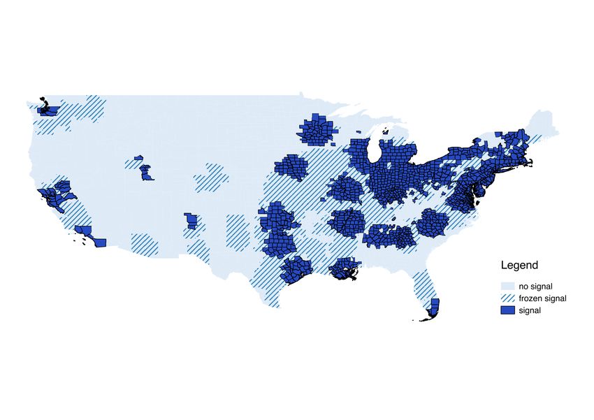

1     Introduction
In a celebrated 1981 article Sherwin Rosen argues that technical change can amplify
inequality at the top of the wage distribution and generate extremely high paid
“superstar” earners. The driving force of such superstar effects are technologies that
facilitate an increase in market scale. Rosen concludes that such technologies enable
“many of the top practitioners to operate at a national or even international scale . . .
[and lead to] increasing concentration of income at the top” (Rosen 1981).1 Superstar
theory has become widely popular since Rosen’s original article, and has been used
to model income inequality in various settings.2 However, credible causal evidence
for superstar effects is lacking and recent advances in empirical methodology have
placed a renewed focus on testing such economic theories with clean identification
strategies.3
    This paper uses a natural experiment to test the superstar model and studies
arguably the most prominent case, the entertainment sector, during the historic
rollout of television.4 Before the launch of television in the middle of the 20th century,
successful entertainers typically had a live audience of a few hundred individuals,
while their audience was an order of magnitude bigger after the launch of television.
In line with superstar effects, I find that this shift resulted in disproportionate income
gains for top entertainers. The launch of a TV station increased the income share of
the top percentile of entertainers by 50%, with much smaller gains for back-up stars
and serious adverse effects for average talents. Employment and incomes declined
sharply below the star level.
    The first part of the paper derives testable predictions from the canonical super-
star model. The theoretical literature has focused on cross-sectional predictions of
superstar-effects, comparing the dispersion of talent to the dispersion of incomes.
    1
      Early version of the superstar theory appear in Tinbergen (1956); Sattinger (1975); Sattinger
(1979).
    2
      See, for example, Kaplan and Rauh (2013); Cook and Frank (1995) for a review of multiple
sectors, Terviö (2008); Gabaix and Landier (2008); Gabaix, Landier, and Sauvagnat (2014) for
CEOs, Garicano and Hubbard (2009) for lawyers, Kaplan and Rauh (2009); Célérier and Vallée
(2019) for finance professionals, and Krueger (2005); Krueger (2019) for entertainers.
    3
      List and Rasul (2011) review the use of field experiments to test labor market theories. In the
context of technical change, Card and DiNardo (2002); Lemieux (2006) famously stressed the need
for clean identification to test skill biased technical change theories, and several subsequent studies
indeed leverage exogenous variation to implement such a test (Bartel, Ichniowski, and Shaw 2007;
Akerman, Gaarder, and Mogstad 2015; Michaels and Graetz 2018).
    4
      Classic studies of superstar effects motivate their analysis with examples from entertainment
(see, e.g., Krueger 2019; Cook and Frank 1995; Rosen 1981).

                                                  1

While such cross-sectional predictions are distinctive, they are difficult to test without
a credible cardinal measure of talent. I therefore present alternative predictions
that focus on changes to inequality and are testable in the absence of data on the
talent distribution. The relevant technologies for superstar effects are “scale related
technical changes” (SRTC) which make large scale production easier.5 Such technical
changes magnify superstar effects and produce characteristic changes in inequality
that are different from other classic models of technical change.6 During SRTC the
most talented workers in the profession (the “superstars”) attract an increased share
of customers at the expense of lower-ranked talents. As a result, the right tail of
the income distribution grows, and incomes become concentrated at the top, while
employment and returns of lower-level talents decline.
       The second part of the paper tests these predictions of the superstar theory. The
government deployment plan of early television stations provides clean variation in a
large SRTC. Entertainer audiences multiplied through television and shows eventually
reached a national audience; however, this transformation took place in stages.7 Shows
on early TV stations were broadcast via airwaves to the local population and in
this pioneering period, technological constraints required TV shows to film near the
broadcast antennas. As a result, filming occurred simultaneously in multiple local
labor markets and provided entertainers a bigger platform in locations where stations
were launched. Pioneering work on the US television rollout in Gentzkow (2006);
Gentzkow and Shapiro (2008) used the staggered rollout process and regulatory
interruptions as a natural-experiment to study the impact on television viewers. I
build on this work and study the effect of television on workers in the entertainment
sector.
       The study uses a difference-in-differences (DiD) analysis across local labor markets
during the staggered rollout. The results show evidence of sharply rising superstar
   5
     Superstar effects also require imperfect substitutability of talent. Entertainment is often used as
a representative case, additionally multiple studies suggest that top talent is also difficult to replace
in several other settings (Huber, Lindenthal, and Waldinger 2020; Sauvagnat and Schivardi 2020;
Azoulay, Zivin, and Wang 2010).
   6
     Influential theories of technical change include skill biased technical change (Autor, Goldin, and
Katz 2020; Autor 2014; Acemoglu and Autor 2011; Autor, Levy, and Murnane 2003; Katz and
Murphy 1992) and routine biased technical change (Autor and Dorn 2013; Acemoglu and Autor
2011; Autor, Katz, and Kearney 2008).
   7
     Mass media (e.g., radio, newspapers and cinema) predates television and could reach a national
audience. The variation in television made additional formats of entertainment scalable, and the
local variation largely unfolds orthogonal to established media formats. In the analysis, I treat the
location of production hubs of the established media as a local fixed effect.

                                                   2

effects. With the launch of a TV station the entertainer income distribution became
more right skewed, with most of the skew happening in the very top tail. The fraction
of entertainers with incomes that reach the top 1% of the US wage distribution
doubled, with smaller increases at slightly lower income levels. Further down in
the distribution such gains disappear quickly and lower-ranked talents lost out.
The share of entertainers with mid-paid jobs declined, and total employment of
entertainers contracted by approximately 13%. Data on consumer expenditure shows
that this is driven by a shift away from traditional live entertainment (e.g., grandstand
shows at county fairs), as returns and audiences for the most successful TV shows
increased strongly. As a result, the income share of the top 1% entertainers increased
approximately 50%. In short, SRTC moved the entertainment industry toward a
winner-take-all extreme, as predicted by superstar theory.
       Two additional sources of variation help to strengthen the identification strategy.
First, I use an unplanned interruption of the television deployment process. During
the interruption, a group of places that were next in line for television had their
permits blocked. Newly collected data on pending regulatory decisions allows me
to track affected places.8 Such places show no evidence of spurious shocks, and
results from placebo tests support the assumption that the television deployment
was exogenous to local demand conditions. Second, I exploit the staggered launch of
TV stations together with the later decline of local filming. The decline provides an
additional difference in the DiD setting and allows me to check if treatment effects
disappear. While the analysis focuses on the rise and fall of local television filming,
nationalized TV stars of course continued to thrive in the subsequent years. Strikingly,
by 1993 entertainers had become one of the 5 most important occupations for the
US top 0.1% income share (Bakija, Cole, and Heim 2012). Today entertainers reach
global audiences and continue to be among the highest-paid individuals in the US
economy.9
       Two “endogeneity challenges” have made it difficult to obtain causal estimates of
the effect of technological change on inequality. A first challenge is that periods of
technical change often coincide with trends in deregulation and shifts in pay-setting
   8
     Previous studies indirectly use this interruption period but lack the data to identify specific
locations held up by the interruption.
   9
     Among the top 0.1% highest-paid Americans, only finance professionals and entrepreneurs
receive higher incomes than entertainers. Entertainers also contribute more to top income shares
than medical professionals or CEOs of publicly traded companies and about the same amount as
engineers, despite the small size of the sector (Based Tables 3a and 7a of Bakija, Cole, and Heim
(2012) and ExecuComp records on the compensation of CEOs of publicly traded companies).

                                                 3

norms, thereby making it difficult to identify the impact of the technical change itself.
In this study, I use industry-specific year effects to absorb the impact of aggregate and
industry level trends and exploit that the television deployment plan affected different
parts of the US at different times. A second challenge concerns the endogenous
adaption of technology. Endogenous adaption can lead to a simultaneity problem
between variation in technology and local labor market shocks.10 In the context of
television, the rollout deployment rules alleviate this problem. The government used
predetermined local characteristics to rank locations in order of priority, thereby
making launch dates unresponsive to local shocks and generating variation that
is exogenous to local economic conditions. The rollout interruption provides an
additional check on this process and we can verify that places where stations failed
to launch do not experience spurious effects around planned launch dates.
    To examine the robustness of results, I probe whether the change in inequality
is driven by television or by other contemporaneous local changes. I find that the
effect of television remains broadly similar when I control for changes in the local
demographic makeup and different trends between urban and rural areas, and even
when controlling for completely flexible differences in linear trends across local labor
markets. Furthermore, I confirm that stations only affect local inequality when
filming is local. The estimates show that local television stations have an impact
in the 1940s and stations seize to have an effect after videotaping eliminates local
filming in the late 1950s. This rise and fall pattern suggests that the effects are indeed
driven by television and rules out that differential linear trends could be driving the
results. Taken together, all these tests confirm that other correlated shocks cannot
explain the rise of entertainer inequality after television launches.
    One potential driver of the change in the wage distribution is a change in the
pool of people who become TV stars. I use panel data and historical records on the
recruitment of TV stars to quantify the importance of this channel and find that it
played only a small roll. TV stations mainly hired the same actors as pre-television
outlets. I also investigate the magnitude of migration responses across local labor
markets and again find very minor effects. These results suggest that changes in the
return to different ranks of talent are the main driver of the observed increase in
inequality.
    This study relates most closely to previous work on superstar effects which found
  10
     For a discussion of endogenous technical change see Acemoglu (1998), and for historical evidence
see Beaudry, Doms, and Lewis (2010).

                                                 4

that this theory could help understand inequality in multiple settings (Cook and
Frank 1995; Krueger 2005; Gabaix and Landier 2008; Terviö 2008; Garicano and
Hubbard 2009; Kaplan and Rauh 2009; Kaplan and Rauh 2013; Gabaix, Landier,
and Sauvagnat 2014; Krueger 2019).11 Such studies find a strong correlation between
top income growth and market reach and argue that superstar effects could explain
this correlation. In this study, I exploit a natural experiment to test the superstar
mechanism and provides evidence for the empirical relevance of such effects.
       More broadly, this study relates to the work on the labor market effects of
technological change. Influential work has analyzed effects on the skill premium
(Autor, Goldin, and Katz 2020; Autor 2014; Acemoglu and Autor 2011; Autor, Levy,
and Murnane 2003; Katz and Murphy 1992) and on routine occupations (Autor and
Dorn 2013; Acemoglu and Autor 2011; Autor, Katz, and Kearney 2008) and used
natural experiments to test these theories (see, e.g., Bartel, Ichniowski, and Shaw
2007; Akerman, Gaarder, and Mogstad 2015; Michaels and Graetz 2018). Evidence
for superstar effects, by contrast, is still scarce.
       Another related literature discusses the link between the market dominance of
superstar firms and market power.12 Both these factors relate to market shares, which
makes it difficult to distinguish their impacts in practice. I use additional variation
to separate the effect of the two and analyze how competition affects the magnitude
of superstar effects. Specifically, I differentiate cases where the television deployment
process leads to a single television station, allowing for scale but no competing
employers, and cases with multiple stations, featuring scale and competition. The
results show marked differences across the two settings. Top incomes only increase
if employers have to compete for talent, while top incomes are nearly unchanged in
locations where a single station operates. As a next step, I estimate rent-sharing
equations that quantify the pass-through of show revenues to entertainer superstars.13
To perform this analysis, I collect additional information on productivity (output
prices, audience sizes and revenues). I use this data in an instrumental variables
  11
     Other work points out that the rise of information and communications technologies may have
created a burst of superstar effects that could help explain why inequality has increased so rapidly
in the wider economy (see, e.g., Cook and Frank 1995; Brynjolfsson and McAfee 2011; Guellec and
Paunov 2017; Kaplan and Rauh 2013).
  12
     Autor et al. (2020) study “superstar firms” and find that the rise in their scale can explain a
decline in the labor share. Studies of monopsony power include, among many others, Van Reenen
(1996); Harmon and Caldwell (2019); Kroft et al. (2020).
  13
     Similar rent-sharing equations have been estimated for construction workers (Kroft et al. 2020),
for patenting firms (Kline et al. 2019) and for CEOs (Gabaix and Landier 2008).

                                                 5

strategy, which instruments show revenues with the launch of television stations and
find that star entertainers receive roughly 1/5 of the additional revenue associated
with the increase in production scale.
         In this paper I focus on the impact of SRTC on the labor market, which of course
is only one aspect of the social consequences of SRTC. For example, SRTC may play
an equalizing force in the marketplace for goods and services. Acemoglu, Laibson,
and List (2014), for example, discuss superstar effects in teaching and highlight that
SRTC could bring higher quality teaching to a greater number of students.
         The rest of the paper is organized as follows: section 2 derives testable predictions
from a canonical superstar model, section 3 discusses the television rollout and data
collection, section 4 presents the empirical results, section 5 analyses the role of
competition, and section 6 concludes.

2         The Superstar Model
This section presents a standard model of the superstar economy and shows how
technical change generates inequality. A superstar economy features heterogeneous
workers (actors) and employers (theaters) of varying sizes. A theater of size s hires
an entertainer of talent t and generates revenue Y (s, t). For simplicity, I assume that
each theater hires only one entertainer and produces revenue:14

                                         Y (s, t) = πφ(st)1/φ ,                                   (1)

where π is the output price and φ is the scalability parameter. A reduction in φ
decreases the curvature of the production function and makes large-scale production
cheaper. Also note that the Cobb-Douglas exponents on s and t are the same, which
may seem like a restrictive assumption; however, when talent t cannot be measured
in a cardinal way, any Cobb-Douglas function can be transformed into this type of
function by changing the units of t. The assumption is thus without loss of generality
and saves on notation. A second important feature of Y is that talented actors have
a comparative advantage in larger shows; in other words Y is supermodular in talent
(Yts > 0).
         The equilibrium is competitive and will meet the social planner optimum, and
we can therefore focus on the optimal allocation. The first equilibrium result follows
    14
         For more general production functions, see Rosen (1981); Tinbergen (1956); Sattinger (1975).

                                                    6

from comparative advantage. Better actors are more valuable in bigger theaters,
and the optimal matching, therefore, requires positive assortative matching (PAM).
Formally PAM implies that a matched actor–theater pair are at the same percentile of
their respective distributions pt = ps . The second equilibrium condition follows from
incentive compatibility. For continuous distributions of talent and theater size, this
requires that wages grow in line with productivity, w0 (t) =              ∂Y
                                                                          ∂t   . Actors and theaters
have outside options that are only infinitesimally worse, and as a result, neither party
earns rents over their outside option (see e.g., Terviö 2008).15 The third equilibrium
                               R1
condition is market clearing ( 0 −Y (s(t), t)dpt = D(π ∗ )), with demand D(π ∗ ) equal
to supply at equilibrium prices π ∗ (for the formal derivation of the equilibrium, see
Online Appendix A.1).
       With these three equilibrium conditions, we can derive the wage distribution.
To obtain a closed-form solution, we additionally assume that talent t and theater
size s follow Pareto distributions, with shape parameters α and β for talent and
                                                                 − β1                    1
theater size, respectively (with inverse CDF pt = t(p)                  and ps = s(p)− α ). Similar
results hold approximately for broader distributional assumptions (see Terviö 2008;
Gabaix and Landier 2008). Combining the incentive compatibility condition with
the production function and integrating gives the wage in the superstar economy:

                                         α+β     1/φ
                    ln(wi ) = ln(λ) +        ln(si ) = ln(λ) + ξ · ln(si ).                        (2)
                                          α
An individual i receives wage wi , which depends on the individual’s audience reach
                                   β
si and the intercept ln(λ) ≡ ln(π α+β ). The effect of audience reach on wages is
       α+β
ξ=      αφ .   Empirical studies have used equation 2 to estimate model parameters and
found that the superstar model closely fits the data in several contexts—for instance,
for CEO compensation (Terviö 2008; Gabaix and Landier 2008).16
       There are at least three challenges with estimating equation 2. A first empirical
challenge is that si is endogenous, and the correlation with wages is unlikely to
produce unbiased estimates of the model parameters. A second challenge is to
                                            1/φ
measure the relevant variation in si              . In the model this parameter represents a
market reach primitive—equivalent to the audience in the entertainment setting—but
  15
      Terviö 2008 concludes: “Due to the continuity assumption, the factor owners do not earn rents
over their next best opportunity within the industry.” This holds even though each actor and show
is a monopolist of its type because of continuity. If the distribution of theater size has jumps, the
theater owner at the jump has market power and could extract all the surplus at that jump.
   16
      These studies implicitly use the first equality of 2, which relates “effective units” of audience
         1/φ
reach (si ) to wages and model primitives.

                                                   7

since this input to the production function is rarely observed directly, studies instead
use proxies such as profits. A concern with this approach is that profits also capture
the endogenous price response and thus lead to biased estimates. A final challenge is
that alternative models could yield a similar correlation of wages and market size.
The correlation thus provides only weak evidence for superstar effects. The following
section provides a framework to tackle these challenges.

2.1       The Effect of Technological Change
To build a more robust test for superstar effects I present additional predictions of
the superstar theory. These predictions leverage the effect of SRTC. The magnitude
of superstar effects is closely linked to the scale of economic production: when scale
economies improve (φ ↓), superstar effects get magnified. The following proposition
summarizes the impact of SRTC (for derivations, see Online Appendix A.2):17

Proposition. In the superstar economy, SRTC leads to
       a) Top wage growth: Denote the share of workers with incomes above a top income
threshold ω by pω ≡ P r(w > ω). SRTC increases pω and more so at higher levels of
                                 0
income: 4ln(pω ) > 4ln(pω ) if ω > ω 0 ;
       b) Fractal inequality: For top income shares (sx ) at two percentiles x and x0 , pay
differences increase: ∆sx0 /∆sx > 1 if x0 > x;
       c) Adverse effects for lesser talents: Employment at mid-pay levels declines; and
       d) Employment loss: For a given outside option wres and corresponding participa-
                                      ∂ p̄
tion threshold p̄, SRTC leads to      ∂φ     < 0.

       The first two results, (a) and (b), state that top earners experience the largest
income growth and income growth rates escalate towards the top of the distribution.18
                                                                                           1
                                                                                          −α
To derive the share of top earners (pω ), combine the size distribution ps = sp                with
equation 2.

                                      log(pω ) = γ0 − γ1ω φ,                                     (3)
  17
     An equivalent SRTC shock could be modeled as an increase in the dispersion in the size
distribution.
  18
     Note that the effects are expressed in terms of the share of entertainers above wage thresholds.
We could alternatively measure wage growth at different percentiles of the distribution. The two
approaches are perfectly interchangeable and the wage distribution provides a direct mapping
between the two. The first approach has empirical advantages and I therefore focus on these results.

                                                    8

βπ                        ln(ω)
where γ0 = ln( α+β   1
                   ) αξ and γ1ω ≡        (α+β)    captures the heterogenous impact of φ at
different wage levels ω. Notice that the coefficient γ1ω is bigger for larger ω, implying
that SRTC (φ ↓) has the biggest impact on the superstars in the economy, while
the impact decreases as we move further down in the distribution (a). A further
implication of this result is that the difference between top income shares increases
(b). The top income share of the top 1% of earners, for instance, rises more than the
the share of the top 10%, a pattern known as “fractal inequality.” A key feature of
these results is that they hold independently of the distributional parameters and we
can thus test for superstar effects without assumptions on the talent distribution.
       The final two results, (c) and (d), capture the winner-take-all nature of superstar
effects and state that mid-income jobs are destroyed and overall employment drops
as markets move towards a winner-take-all setting. This effect operates through
declines in entertainment prices π. A simple case of falling π arises with completely
inelastic demand—in this case, the rising scale of stars directly reduces demand
for other workers, but more generally the winner-takes-all phenomenon arises when
the demand is sufficiently inelastic.19 The declining price affects the value of the
intercept (γ0 ) in equation 3. This intercept affects wages at all percentiles equally,
but it carries a bigger weight at lower wage levels, where the benefit from scale (γ1ω )
is small. As a result, SRTC benefits stars, while lower-ranked workers suffer from
falling demand for their services. Workers whose wage drops below the reservation
wage exit entertainment and employment therefore falls.
       The effects of SRTC are summarized in Figure 1. The figure shows how wages
in entertainment are predicted to spread out relative to the rest of the economy:
Extreme pay becomes more common, while the share of mid-income jobs declines.
Notice that Figure 1 shows bins that get narrower at the top of the distribution in
order to zoom in on the part of the distribution that is most affected. The impact
at the top resembles an upward pointing hockey stick, with the sharpest effects at
the very top and declining impacts at lower income levels. At the bottom of the
distribution, the figure shows a case where SRTC decreases the lower bound of the
wage distribution, which in turn results in a growing low paid sector and an increased
share of workers at the lowest income levels.20
  19
    See Appendix A.2 for further details on this demand condition.
  20
    Effects at the bottom of the distribution are more sensitive to assumptions. A case with a
uniform reservation wage and no adjustment costs, for instance, implies that the lower bound of the
wage distribution is fixed at the reservation wage. Demand shifts then only affect employment and
do not change wages of low paid workers.

                                                  9

It is useful to compare these effects to alternative models of technical change.
Superstar effects differ from a large class of alternative models. The canonical model
of skill biased technical change, for example, features only two skill groups and thus
produces little top income dispersion. Even extensions to SBTC models will struggle
to generate top income inequality, particularly of the fractal nature described above.
To replicate fractal inequality with SBTC, we would need to get rid of the groups of
perfectly substitutable workers and introduce imperfect substitution between workers.
This is in principle feasible by taking the number of skill groups to infinity. Such
an approach, however, is unattractive, as it introduces infinitely many parameters
and makes the model impossible to falsify. The superstar economy instead provides
a parsimonious and thus falsifiable model of income inequality. A second challenge
for models with labor augmenting technical change is to generate real wage and
employment losses (Caselli and Manning (2019)). The superstar framework produces
such losses naturally, as shown by (c) and (d).
   An alternative class of technical change models has introduced task-specific
technical change (for a summary of task based models, see Acemoglu and Autor
(2011)). Such models have similarities to the superstar framework in that the latter
also uses an assignment process to assign workers to tasks (or stages in our case).
The task framework can produce real wage declines in response to labor augmenting
technical progress by shifting workers into other tasks and increasing the supply of
workers to such tasks. When it comes to top-income dispersion, task models face
similar limitations to SBTC: Workers of equal skills are perfect substitutes and wage
dispersion thus arises across skill groups only. We can generate a task model that is
near isomorphic to a superstar model by letting the number of tasks and skill groups
approach infinity. This generates one-to-one matching between tasks and worker
types, just like the superstar model. A remaining difference is how the two models
conceptualize technical change. The task model has been used to study the impact
of factor augmenting shocks, or changes in the tasks performed by workers. Factor
augmenting shocks can produce fractal inequality if we assume that the technological
shock is fractal itself, in the sense that technology boosts productivity most for
the highest productivity workers. And while it is thus possible to generate fractal
inequality, we would practically assume the conclusion that we generate. In the
superstar framework technical change (SRTC) affects a different parameter (the scale
parameter) and the effect on labor demand at different skill levels arises endogenously,
producing fractal inequality.

                                          10

3         Data and Setting
To take these predictions to the data, I build a novel data set that covers the
entertainment sector during the middle of the 20th century. I combine historical
records from multiple archival sources to track the locations of technological change,
the resulting shift in market reach, and labor market outcomes. In addition, I collect
information on administrative rules to isolate plausibly exogenous variation in the
television rollout process.

3.1        Television Rollout
At the start of the 20th century, local live shows—particularly vaudeville shows,
the legitimate stage, and county fairs—were among the most popular forms of
entertainment. Vaudeville shows typically featured a variety of acts, including
comedy, stunts, acrobatics, ballet, burlesque and dance, while the legitimate stage
presented drama and theatrical plays. The local entertainment sector changed quickly
with the launch of television in the 1940s and 1950s. Through television traditional
stage entertainment could reach an audience multiple times the size of a live show
and began to reach mass audiences.
         Early TV stations predominantly filmed their own content and broadcast local
shows via airwaves to the local area. This fragmentation of filming was the result
of technological and regulatory constraints of the early period of television. The
most important reason was the lack of infrastructure to transmit shows from station
to station (see Sterne (1999) for a detailed account). A second constraint was that
recording technologies were in their infancy and resulted in poor image quality. As a
consequence, recorded shows were a poor substitute for local live television shows.21
Finally, regulation also imposed restrictions on studio locations and required that
“the main studio be located in the principal community served.” 22 As a result, TV
studios were scattered across the country and the launch of a local TV station implied
the launch of local filming.
         In order to track the rollout, I digitize archival records of TV stations published
in “Television Digest” reports and match station addresses to local labor markets.
This broadly follows the strategy of Gentzkow (2006); Gentzkow and Shapiro (2008)
    21
     Non-local content had to be put on film and shipped to other stations, where a mini film
screening was broadcast live. This was known as “kinescope.”
  22
     See FCC Rules & Regulations, Section 3.613 (version May 1952)

                                               11

who study variation in TV signal during the roll-out process. Television filming
started in the early 1940s, and Figure 2 shows television filming by the time of the
US population Census in 1949. At this point 62 stations were active, and the Figure
shows where they were located.23 In the following decades the number of stations
grew substantially, but by the mid-1950s local stations started to lose their relevance
for filming. This rise and fall of local television filming will provide the basis for a
DiD analysis that compares local labor markets during the launch and subsequent
decline of local filming.
       An unplanned interruption of licensing in 1948 creates a natural experiment that
strengthens the identification strategy. During the interruption a group of locations
that would have received television narrowly missed out on television launches. The
data on the affected places comes again from “Television Digest” which includes
a supplement that reports on ongoing permit decisions of the FCC.24 To exploit
the variation from this interruption, I define a “rollout interruption sample” which
narrows in on 113 CZs which either had television at the time of the interruption or
missed out on television launches because of the interruption.
       The principal reason for the rollout interruption was an error in the FCC’s
airwave propagation model. This model was used to delineate interference-free signal
catchment areas, but the error implied that signal interference occurred between
neighboring stations. To avoid a worsening of the situation, the FCC put all licensing
on hold and ordered a review of the model. Previous studies noted this interruption
but lacked the records to identify locations that where held up by the FCC. I collected
new data to distinguish such locations from late adopters, and show were blocked
stations are located in Figure 2. Licensing only resumed in 1952, delaying the onset
of television by at least four years in the affected locations.25
       After the initial rollout, local television filming eventually declines. The main
driver of this decline was the invention of the Ampex videotape recorder which made
  23
     I assume that all stations were filming locally at that time. A handful of stations are an
exception and operated a local network. This was rarely feasible because the technical infrastructure
was still in its infancy. In my main specifications, I code all members of such networks as treated to
avoid potential endogenous selection of filming locations within the network.
  24
     I use the “TV Directory” No. 6 of January 1949 to identify places affected by the interruption.
All places where the FCC had started vetting potential licensees (“applicants”) at this time are
coded as affected by the interruption.
  25
     The timing of the interruption (1948–1954) coincides with the 1950 US decennial Census which
makes it possible to investigate the labor market consequences in detail. Initially, the interruption
was expected to last a year. However, the review was delayed to ensure compatibility with rising
new transmission technologies (UHF and color transmission).

                                                 12

recorded shows a close substitute for local live shows. Once videotaping was possible,
stations increasingly substitute away from local filming. This decline of local filming
provides an additional check for the analysis, as the impact of local station should
fade as local filming declines. The videotape recorder was first presented at a trade
fair in 1956, and immediately more than 70 videotape recorders were ordered by TV
stations across the country. That same year, CBS started to use the technology, and
the other networks followed suit the next year, resulting in the rapid decline of local
filming. In subsequent years television filming started to concentrate in two hubs,
Los Angeles and New York, and declined in other locations.26 During this videotape
era, we have to account for the emergence of national filming hubs and regressions
will include fixed effects for hubs in the post-videotape period. To avoid a potential
endogenous control issue, I do not control for filming hubs directly but use a proxy
for comparative advantages of a location as a filming hub. These proxies are based on
a location’s fixed characteristics, such as sunshine hours and landscapes, that largely
drove location decisions. I quantify such predetermined factors using the share of
movies filmed in the local labor market in 1920.27

3.2      Labor Market Data
Data on labor market outcomes are based on multiple historical sources. The first set
of outcomes comes from the microdata samples of the decennial US Census (1940–
1970). I focus on five entertainment occupations that benefited from the introduction
of TV: actors, athletes, dancers, musicians, and entertainers not elsewhere classified
and track their labor market outcomes across the 722 local labor markets that span
the mainland US.28 The Census first collected wage data in 1940, and in all years
asked about annual wage income in the previous year; wages reported in 1940 thus
refer to 1939.29 The wage data is top-coded, but fortunately, the top code bites
above the 99th percentile of the wage distribution, and up to that threshold, detailed
analysis of top incomes is possible.
       To evaluate the predictions of the superstar model, I compute several inequality
  26
     This trend was also helped by the contemporaneous rollout of coaxial cables that allowed
producers to relay live shows from station to station.
  27
     The historic location data of movie filming comes from the online Internet and Movie Database
(IMDb).
  28
     I follow Autor and Dorn (2013) and define local labor markets based on commuting zones (CZ).
  29
     The Census reports wage income in all sample years, while business income is not consistently
available. I therefore focus on wage incomes.

                                               13

metrics at the local entertainer labor market level. A first set of outcomes focuses on
the rank of local entertainers in the US income distribution. I first compute the share
of local entertainers that reaches the top 1% of the US income distribution.30 The
value goes from 0 when no entertainer earns such extreme to 100 in a winner-takes-all
market with a single superstar entertainer.31 The share in market m at time t is
given by                                        P
                                         99            Ei,m,t
                                      pωm,t =     iI
                                                              ,                                  (4)
                                                      Et
where E is a dummy that takes the value 1 for entertainer occupations and I is
the set of workers in the top 1% of the US wage distribution. The wage top code
bites above the 99th percentile of the US distribution and we can thus identify all
workers in the top 1%.32 A potential issue with these shares is that fluctuations in
the denominator can generate spurious effects. To prevent this, I use the number of
entertainers in the average labor market (Ēt ) as denominator instead of local labor
market counts.33 As an alternative approach, I compute per capita counts which
use the local population as the denominator. These measure map directly into the
predictions derived in section 2 and measures how the top tail of the entertainer
distribution stretches out relative to the US distribution. We can naturally extend the
analysis to other percentiles and study where entertainers rank in the US distribution
across all income ranges. Finally, I also compute the wage at the top percentile of
the local entertainer distribution and top income shares of local entertainers.
       I complement this data on local inequality with a small panel on the work history
of TV superstars. The large amount of fan interest generates unusually detailed
records on the background of this group and makes it easier to identify and track the
history of entertainer stars. The data on TV stars comes from the 1949 “Radio and
Television Yearbook” which publishes an annual “Who is Who” in television—a list of
stars similar to modern Forbes lists. The data covers the top 100 or so most successful
  30
     This metric is similar in spirit to Chetty et al (2017) who also study ranks of local workers in
the national distribution. The authors highlight that such ranks have advantages over income levels
for comparisons over longer time periods.
  31
     In the baseline estimates, I code areas without local entertainers – for instance areas where
television displaced all local entertainers – as 0.
  32
     The relevant top 1% thresholds are: 7,555 8,050 11,859 16,247 in 1950 USD for 1940, 1950, 1960
and 1970 respectively.
  33
     To interpret the estimates as percentage point changes, I normalize by the average number of
                                                                                            99
entertainers in treated labor markets. Note that this normalization also implies that pω   m,t can in
principle be bigger than 100. For robustness, I also run the regressions without the normalization
and find similar results (for more details, see Appendix B5).

                                                 14

TV entertainers and their demographic information (e.g., names, TV station employer,
birthdays and place of birth) but not income. To obtain information on their pre-TV
careers, I link this data to de-anonymized records of the 1940 Census. This link is
based on names and additional demographic information (e.g., place of birth, birth
year, parental information) and I can uniquely identify 59 of these TV superstars in
the Census.34 While the data is inevitably imperfect, it offers a rare window into the
background of the stars of a profession and allows me to study the background of the
group that benefitted most from the SRTC of television.
       To measure the effect of TV on traditional live entertainment, I collect additional
data on attendance and spending at county fairs. The data cover annual records of
revenues and ticket sales for more than 4,000 county fairs over 11 years (1946–1957)
and spans most US local labor markets. I collect these records from copies of the
“Cavalcade of Fairs,” an annual supplement to Billboard magazine and compute
spending at local fairs for three spending categories that are differentially close
substitutes for television: spending on live shows (e.g., grandstand shows), fair
entrance tickets, and carnival items (e.g., candy sales and fair rides). Live shows
most closely resembled TV shows at the time, while candy sales and fair rides are by
nature less substitutable with TV.
       Finally, I trace where and when county fairs faced competition from TV shows.
Figure 3 shows where TV was available in 1950, based on TV signal data from Fenton
and Koenig (2020). The year 1950 falls in the period of the rollout interruption,
and hence a number of places that were meant to have TV did not yet. Records of
technical features of such stations allow me to reconstruct where such stations would
have broadcast, and these locations are also illustrated in Figure 3.

3.3      Audience and Revenue Data
The entertainment setting offers a unique opportunity to quantify the market reach of
workers by measuring show audience sizes. I collect data on audiences and revenues
of live and TV shows from archival records. For live shows I use the venue capacity
reported in the 1921 Julius Cahn-Gus Hill Theatrical Guide. This guide claims to
provide “complete coverage of performance venues in US cities, towns and villages”
  34
    To maximize the match rates of the “Who Is Who” and Census data, I supplement the available
demographic information with hand-collected biographic information from internet searches. As a
result, I achieve a 70% unique match rate among the 68 records with birth-year information, while
a few cases are matched without birth-year information.

                                               15

and covers over 3,000 venues across roughly 80% of local labor markets.35 For TV
shows I compute the number of TV households in a station’s signal catchment area.
This uses TV ownership data from the Census and signal data from Fenton and
Koenig (2020). I also collect price information from TV stations’ pricing menus, the
so called “rate cards,” and compute the revenue of local shows. TV shows provided
an enormous step-up in the revenue and audience of entertainment shows.36 Before
television, live shows reached on average 1,165 people, while the median TV station
could reach around 75,000 households.
         Additional details on the data collection, the data processing and summary
statistics are available in Online Appendices B.1 and B.3.

4         Empirical Results
The distribution of incomes in entertainment was far more equal in 1939 than it is
today. Figure 4a shows the income distribution among entertainers before television,
in 1939, and after the rise of television, in 1969. Over this period pay dispersion
grew substantially: wages at the top grew disproportionately, many mid-income jobs
disappeared, and a larger low-paid sector emerged. At the same time, employment
growth in performance entertainment lagged behind the employment growth in other,
non-scalable, leisure-related activities, e.g., restaurant and bar workers, fountain
workers, and sport instructors (Figure 4b). This pattern of rising dispersion in log
pay and the lack of employment growth is precisely what characterizes superstar
effects. Yet from these aggregate patterns it is unclear whether the rise of television
during this period is just a coincidence or is driving these effects.
         I use a DiD regression across local labor markets to identify the effect of television.
The variation comes from the local deployment of TV stations during the 1940s and
early 1950s and from the subsequent demise of local filming in the mid-1950s. I
track changes in the local entertainer wage distribution during this period. I run the
regression at the a disaggregated labor market (m), year (t), occupation (o) level
    35
     According to the guide, “Information has been sought from every source obtainable–even from
the Mayors of each of the cities” (p. 81). Undoubtedly the coverage was imperfect and small or
pop-up venues were missed, but since we focus on star venues these omissions may be of lesser
concern. I use the largest available audience in the local labor market to proxy for a star’s show
audience. I probe the reliability by manually comparing specific records with information from
archival data, and the data seem reliable.
  36
     For details on revenue data, see Online Appendix B.3. For TV shows, prices are imputed based
on estimates of the demand elasticity in a subset of 451 markets where data are available.

                                                 16

and control for occupation-year fixed effects to capture potential time fluctuations
in the occupation definition. The athlete occupation, for instance, is subsumed in
the nec entertainer category in 1960. The standard errors mot are clustered at the
local labor market level so that running the analysis at the disaggregated level will
not artificially lower standard errors. The full sample thus includes 722 local labor
markets, 5 occupation groups and 4 Census years (2 for athletes) and hence uses
13,718 observations and 722 cluster:

                     Ymot = αm + δot + γXmt + βT Vmt · Dtlocal + mot .                            (5)

Ymot measures labor market outcomes (e.g., the share of entertainers in the top 1%
of the wage US distribution), αm and δot are labor market and occupation specific
year fixed effects, and Xmt is a vector of control variables and includes the control
for filming hubs of the post-videotape period. The treatment variable, T Vmt , is the
number of local TV stations, and Dtlocal is a dummy that takes the value 1 when TV
stations film locally, before the rise of the videotape recorder in 1956. T Vmt thus
captures the staggered rollout, while Dtlocal captures the eventual decline of local
filming. In addition to a standard DiD set-up, we here observe both the rollout and
the removal of local TV filming and thus have access to a third “diff” that helps with
identification.
       Consider how the variation in T Vmt relates to previous production technologies.
Before television radio, newspapers, and movies where already popular mass-media
formats and the time invariant effects of pre-existing production hubs will be absorbed
by fixed effects. Additionally, note that we would not be able to detect effects of
television if entertainers’ audience reach was unaffected by the launch of television.37
In practice, television produced a sharp shift in audiences – which we will discuss in
detail below – and this shift provides sufficient power to pick up superstar effects.38
       A major advantage of this setting is that a government deployment process drives
variation in T Vmt . The government deployment rules generate variation in TV that
is orthogonal to local demand shocks. This deployment process therefore breaks the
  37
     The validity of the test would be unchanged but the power of the test would be reduced.
  38
     Television expanded audiences for two principle reasons: First, new entertainment formats
became scalable, particularly ones that relied on visual broadcasts. The study focuses on the group
of entertainer occupations that were mainly affected by the launch of television. Second, the regional
variation of the rollout is largely orthogonal to existing hubs. In places with pre-existing hubs, the
permanent effects will be absorbed by location fixed effects and the impact of television is identified
through local changes in inequality.

                                                  17

direct link between local economic conditions and television launches and avoids the
simultaneity problem that arises from ordinary, endogenous technology adoption.
       There is, however, still potential for endogenous variation if the government
decisions themselves are influenced by local demand conditions. I investigate this
possibility in archival records of the government decision rules. These records show
that decisions rules were indeed independent of local demand and fairly rigid. The
1952 “Final Television Allocation Report,” for instance, prioritized locations by their
local population in 1950 and the distance to the nearest antenna.39 The government
priority ranking is thus based on pre-determined location characteristics and is by
construction unresponsive to local demand shocks.
       A further advantage of this setting is the rare use of television outside the
entertainment industry. Television was hardly ever used in other industries. Many
similar SRTCs, by contrast, simultaneously affect multiple sectors and thus generate
several simultaneous changes that make it difficult to identify superstar effects. The
near exclusive use of television in entertainment makes this setting a particularly
clean case of SRTC.

4.1      Results: Rising Returns at the Top
The first set of tests study Proposition (a) and tests the impact of SRTC on the top
of the income distribution. A first outcome is the share of entertainers among the
top 1% highest-paid Americans.40 Growing right skew of the distribution implies
that the share of entertainers at such extreme income levels increases. Indeed, a
local TV station roughly doubles the share of local entertainers in this income group,
increasing the size of this group by about 4 percentage points (Table 1, Panel A).
       Similar results hold for the number of top-paid entertainers per capita (Panel B).
These estimates confirm prediction (a) and show that TV creates a group of extremely
highly compensated entertainers. The gains among top entertainers are particularly
remarkable in the context of the historical period. Top income growth in the overall
economy was low in the mid-20th century and the growth among entertainers thus
stand out.
  39
    Published as part of the FCC’s Sixth Report and Order (1952)
  40
    Top earners in entertainment were notably more diverse than other sectors. Women made
up 15% and non-white minorities 1.5% of top earners, while other high-paid occupations where
essentially closed to women and minorities. Less than 2% of top paid managers, lawyers, medics,
engineers and service sector professionals were women and less than 0.5% where from minority
groups.

                                              18

A potential identification concern are differential local trends. As a first pass,
I use two specifications to check for such effects. The first specification, column 2,
adds control variables that proxy for local economic changes (i.e., local median age
and income, % female, % minority, population density, and trends for urban areas).
These estimates yield very similar results. The second specification, column 3, is
less parametric and allows for location-specific time trends. Such a specification will
capture differences in local trends, independent of their source. It is a very demanding
specification that adds more than 700 coefficients and while standard errors increase,
the results remain remarkably close to the baseline. Both results thus indicate that
differential local trends are not driving the findings.
       Finally, in Panel C I restrict the sample and compare places with television to
places that narrowly missed out on television launches during the roll-out interruption
(the “rollout interruption sample”). The advantage of this approach is that it drops
more rural areas from the analysis and makes the control group more similar to the
treated areas.41 Results with this sample are very similar to the baseline results and
suggest that the previous estimates based on the general roll-out rules are valid.

The Rollout Interruption

The key identification assumption of the DiD is that TV launch dates are unrelated to
local shocks or trends. The previous results with added local trends alleviate concerns
about spurious local trends, but we may still worry about shocks in unobservable
variables that are not captured by these controls.
       The interruption of the television rollout provides a powerful test for such spurious
effects. Recall that all planned launches were blocked in an indiscriminate fashion
and this interruption thus generates variation that is independent of local economic
conditions. We can test if spurious effects arise at the time of planned television
launches and thus check if the rollout process is correlated with local labor market
shocks. Figure 5 plots the number of approved TV licenses over time and shows the
sudden drop in approvals at the time of the interruption. I use such places for a
placebo test that compares untreated and blocked locations. This is implemented in
a dynamic DiD regression that uses blocked stations (T Vmt
                                                        blocked ) as treatment:

  41
    Note that differences between treatment and control areas are not necessarily a problem for
identification as location fixed effects will account for time-invariant differences. More broadly, the
weighted regressions give relatively little weight to less populated observations, which implies that
such observations don’t matter much for the results.

                                                  19

X
                    Ymot = αm + δot + γXmt +                   blocked
                                                         βt T Vmt      + mot .                (6)
                                                     t

Here, βt captures spurious shocks in places that were meant to be treated but narrowly
missed out. Figure 6a plots these coefficients and shows a strikingly parallel trend.
Blocked locations show no sign of spurious changes neither before, after, or during
the time of blocked launches. These results are precisely estimated and rule out even
relatively small violations of the parallel trends assumption. This result also confirms
that the rollout rules, which did not take local demand condition into account, were
followed through in practice. Also notice that this result goes beyond conventional
pre-trend checks. Pre-trend checks focus on trends before the treatment, but with
the blocked station experiment, we can additionally test for spurious shocks at the
time of and after the planned TV launch date. For completeness, I also perform
alternative robustness checks with placebo occupations (Online Appendix B.2.1) and
conventional pre-trends (Online Appendix B.2.2) and both also find no spurious
effects.
       We can additionally test parallel trends within treated labor markets by comparing
the period before the launch of television and after the decline of local television.
Such a test is similar to a pre-trend test but additionally leverages that we observe
the removal of local filming. We can probe whether the treatment effect arises and
disappears with the rise and fall of local filming. I implement this test in a dynamic
DiD regression, using equation 6 with local TV filming as the treatment variable.
The results confirm the expected pattern; differences between treated and untreated
areas appear when TV stations are launched, and disappear again as such stations
lose their importance for filming (Figure 6b plots βt ). In 1969 differences between
treatment and control groups reverted to the pre-treatment level.42 This finding
again supports the parallel trend assumption and rules out even relatively complex
deviations from parallel trends. For instance, exponential and linear growth rates
might look similar at the start of the trends and pre-trend checks might not pick up
any differences. By leveraging the post treatment period, we can check for spurious
differences that only emerge in the longer run and can thus rule out such non-linear
differential trends.
  42
     National filming hubs emerged in this period and those locations saw fast top income growth in
this period (results for hubs are available upon request).

                                                20