Evolution and application of digital technologies to predict crop type and crop phenology in agriculture
←
→
Page content transcription
If your browser does not render page correctly, please read the page content below
in silico Plants Vol. 3, No. 2, pp. 1–23
doi:10.1093/insilicoplants/diab017
Advance Access publication 21 May 2021
Review

      Evolution and application of digital technologies to
      predict crop type and crop phenology in agriculture
      Andries B. Potgieter1,* , , Yan Zhao1, Pablo J. Zarco-Tejada2, Karine Chenu1, ,

                                                                                                                                                                                            Downloaded from https://academic.oup.com/insilicoplants/article/3/1/diab017/6279904 by guest on 22 September 2021
       Yifan Zhang1, Kenton Porker3, Ben Biddulph4, Yash P. Dang1, Tim Neale5,
                           Fred Roosta6 and Scott Chapman7
      1
       The University of Queensland, Queensland Alliance for Agriculture and Food Innovation, Centre for Crop Science, Gatton, Queensland 4343, Australia
  2
   School of Agriculture and Food (SAF) and Faculty of Engineering and Information Technologies (FEIT), The University of Melbourne, Melbourne, Victoria
                                                                         3010, Australia
    3
     The University of Adelaide, South Australia Research and Development Institute, and School of Agriculture, Food & Wine, Crop Sciences, Urrbrae, South
                                                                    Australia 5064, Australia
                4
                  Department of Primary Industries and Regional Development, 3 Baron-Hay Court, South Perth, Western Australia 6151, Australia
                                    5
                                     Data Farming Pty Ltd, P.O.Box 253, Highfields, Toowoomba, Queensland 4352, Australia
                             6
                              The University of Queensland, School of Mathematics and Physics, Brisbane, Queensland 4072, Australia
                           7
                            The University of Queensland, School of Agriculture and Food Sciences, Gatton, Queensland 4343, Australia
                                                  *Corresponding author’s email address: a.potgieter@uq.edu.au

                                                                              Handling Editor: Steve Long

    Citation: Potgieter AB, Zhao Y, Zarco-Tejada PJ, Chenu K, Zhang Y, Porker K, Biddulph B, Dang YP, Neale T, Roosta F, Chapman S. 2021. Evolution and
  application of digital technologies to predict crop type and crop phenology in agriculture. In Silico Plants 2021: diab017; doi: 10.1093/insilicoplants/diab017

                                                                                    A B ST R A C T
                  The downside risk of crop production affects the entire supply chain of the agricultural industry nationally and glob-
              ally. This also has a profound impact on food security, and thus livelihoods, in many parts of the world. The advent of high
              temporal, spatial and spectral resolution remote sensing platforms, specifically during the last 5 years, and the advance-
              ment in software pipelines and cloud computing have resulted in the collating, analysing and application of ‘BIG DATA’
              systems, especially in agriculture. Furthermore, the application of traditional and novel computational and machine learn-
              ing approaches is assisting in resolving complex interactions, to reveal components of ecophysiological systems that were
              previously deemed either ‘too difficult’ to solve or ‘unseen’. In this review, digital technologies encompass mathematical,
              computational, proximal and remote sensing technologies. Here, we review the current state of digital technologies and
              their application in broad-acre cropping systems globally and in Australia. More specifically, we discuss the advances in (i)
              remote sensing platforms, (ii) machine learning approaches to discriminate between crops and (iii) the prediction of crop
              phenological stages from both sensing and crop simulation systems for major Australian winter crops. An integrated solu-
              tion is proposed to allow accurate development, validation and scalability of predictive tools for crop phenology mapping
              at within-field scales, across extensive cropping areas.

              K E Y W O R D S : Big data, crop modelling, digital technologies, drone, food security, machine learning, precision
              agriculture, satellite imagery, subfield scale, UAV.

  1. I N T R O D U C T I O N : S E N S I N G O F C R O P                                          production (>60 % of the current) by 2050 (Alexandratos and Bruinsma
T Y P E A N D C R O P P H E N O L O G Y F R O M S PA C E                                          2012) is one of the greatest tests facing humanity. It is also apparent that
With the burgeoning challenges that Earth is currently experiencing,                              gains in future production are more likely to come from closing the yield
mainly caused by the progressively increase in climate extremes, rapid                            gap (increase in yield) rather than an increase in harvested area. For exam-
population growth, reduction in arable land, depletion of, and competi-                           ple, from 1985 to 2005 production increased by 28 %, of which a main
tion for, natural resources, it is evident that the required increase of food                     portion (20 %) came from an increase in yield (Foley et al. 2011). The

© The Author(s) 2021. Published by Oxford University Press on behalf of the Annals of Botany Company.
This is an Open Access article distributed under the terms of the Creative Commons Attribution License (https://creativecommons.org/licenses/by/4.0/), which permits unrestricted
reuse, distribution, and reproduction in any medium, provided the original work is properly cited.                                                                                  •   1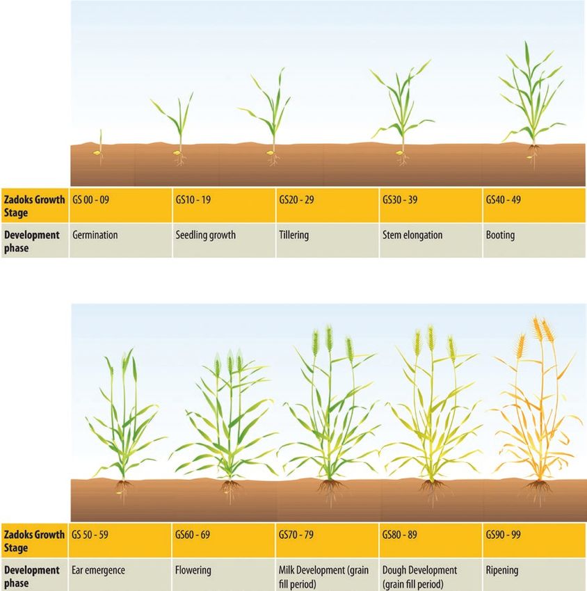
2   •   Potgieter et al.

challenge to produce more food more effectively is so significant that, in    latest long-term simulations studies that define the optimal flowering
2016, ‘End hunger, achieve food security and improved nutrition and pro-      periods. For example, final yield correlates strongly to the optimum
mote sustainable agriculture’ was selected as the second most important,      flowering time (OFT) for sorghum (Wang et al. 2020) across differ-
Sustainable Development Goal (‘End Poverty’ was ranked first) by The          ent environments of north-eastern Australia (Fig. 1). Note that in low
United Nations (https://www.un.org/sustainabledevelopment/).                  rainfall years (2017), this correlation can become negative as later
     Therefore, significant advances in global food production are            flowering crops exhaust the stored water supply. Significant relation-
needed to mitigate the projected food demand driven by rapid popula-          ships were evident for wheat (Fig. 2) (Flohr et al. 2017), canola (Lilley
tion growth and affluence of emerging economies (Ray et al. 2012).            et al. 2019) and barley (Liu et al. 2020) across south-eastern Australia
Furthermore, climate variability and change, especially the frequency         when the OFT is determined across multiple years. For example, in the
of extreme events, in conjunction with regional water shortages and           cooler high rainfall zone at Inverleigh (Fig. 2) the OFT is narrower and

                                                                                                                                                           Downloaded from https://academic.oup.com/insilicoplants/article/3/1/diab017/6279904 by guest on 22 September 2021
limits to available cropping land are factors that influence crop produc-     later compared to Minnipa.
tion and food security (Fischer et al. 2014; IPCC 2019; Ababaei and               Whilst optimization of flowering times has allowed the combined
Chenu 2020). Therefore, accurate information on the spatial distribu-         stresses of drought, frost and heat to be minimized, these abiotic
tion and growth dynamics of cropping are essential for assessing poten-       stresses still take a large toll on crops every year (Zheng et al. 2012a;
tial risks to food security, and also critical for evaluating the market      Hunt et al. 2019). Growers often need to adjust crop inputs to reflect
trends at regional, national and even global levels (Alexandratos and         yield potential and implement alternative strategies such as cutting
Bruinsma 2012; Orynbaikyzy et al. 2019). This is extremely important          frosted crops for fodder. Furthermore, yield losses from these events
for crops growing in arid and semi-arid areas, such as Australia, where       are often spatially distributed and dependent on the phenology stage.
the cropping system is highly volatile due to the variability in climate      Not only does frost events vary spatially with topography across the
and frequent extreme weather events including extended droughts and           landscape from season to season (Zheng et al. 2012a; Crimp et al.
floods (e.g. Chenu et al. 2013; Watson et al. 2017). Indeed, Australia has    2016), but it is also expected there will be more hot days and fewer
one of the most variable climates worldwide with consequent impact            cold days in future climates across much of the cereal belt (Collins
on the productivity and sustainability of natural ecosystems and agri-        et al. 2000; Collins and Chenu 2021). However, frost is still expected
culture (Allan 2000). In addition, cereal yields have plateaued over the      to remain a concern in affecting crop production in future climates
last three decades in Australia (Potgieter et al. 2016), while volatility     (Zheng et al. 2012a). The additional interaction of temperature, water
in total farm crop production is nearly double that of any other agri-        stress and variable soil moisture can lead to large spatial variability in
cultural industry (Hatt et al. 2012). In this regard, digital technologies,   cereal yields (e.g. wheat, barley, canola, chickpea and field pea) with
including proximal and remote sensing (RS) systems, have a critical           regional differences. The crop phenology when stress occurs can also
and significant role to play in enhancing food production, sustainabil-       further exacerbate the spatial and temporal differences in yields (Flohr
ity and profitability of production systems. The application of digital       et al. 2017; Dreccer et al. 2018a; Whish et al. 2020).
technologies has rapidly grown over the last 5 years within agriculture,          Accurate assessment of plant growth and development is there-
with the prediction of a growth in production to at least 70 % at farm        fore essential for agronomic management particularly for the deci-
level, and to a total value of US$1.9 billion (Igor 2018).                    sions that are time-critical and growth stage-dependent in order to

1.1 Linking variability in crop development to yield
Crop growth and development are mainly a function of the interac-
tions between genotype, environment and management (G × E × M).
This can result in large-scale variability of crop yield, phenology and
crop type at subfield, field, farm and regional scales. In most cases,
the environment, including climate and soils, cannot be changed and
matching crop development progress to sowing date and seasonal
conditions is critical in order to maximize grain yield, especially in
more marginal environments (Fischer et al. 2014; Flohr et al. 2017).
Producers can increase yields by choosing an elite yielding variety
adapted to their environment and/or changing cropping practices to
align with expected climatic conditions and yield potentials (Fischer
2009; Zheng et al. 2018). Sowing dates and cultivars are targeted in
each region so that flowering coincides with the period that will mini-
mize abiotic stress, such as frost, water limitation and/or heat known
as the optimal flowering period (Flohr et al. 2017). Despite agro-
nomic manipulation with sowing date and cultivar choice there is still
often significant spatial and temporal variation in crop development          Figure 1. Sorghum yield for 28 commercial cultivars versus
between and within cropping regions and at the field scale.                   days to flowering across three seasons at different locations
    The variability in crop development and its link with grain yield         across north-eastern Australia. Adapted from Wang et al.
across regions and from season to season is captured best by the              (2020) for sorghum.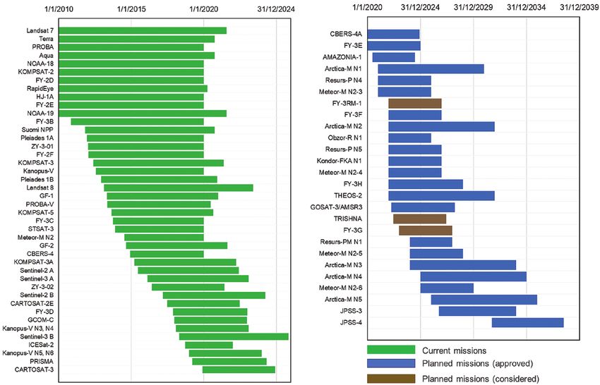
Application of digital technologies in agriculture • 3
Downloaded from https://academic.oup.com/insilicoplants/article/3/1/diab017/6279904 by guest on 22 September 2021
Figure 2. The optimal flowering period (OFP) for a mid-fast cultivar of wheat determined by APSIM simulation for (A) Waikerie,
South Australia; (B) Minnipa, South Australia; (C) Yarrawonga, Victoria; (D) Inverleigh, Victoria; (E) Urana, New South Wales;
(F) Dubbo, New South Wales. Black lines represent the frost and heat limited (FHL) 15-day running mean yield (kg ha−1). Grey
lines represent the standard deviation of the FHL mean yield (kg ha−1). Grey columns are the estimated OFP defined as ≥95 % of
the maximum mean yield from 51 seasons (1963–2013). Data source: Flohr et al. (2017). Image: Copyright © 2021 Elsevier B.V.
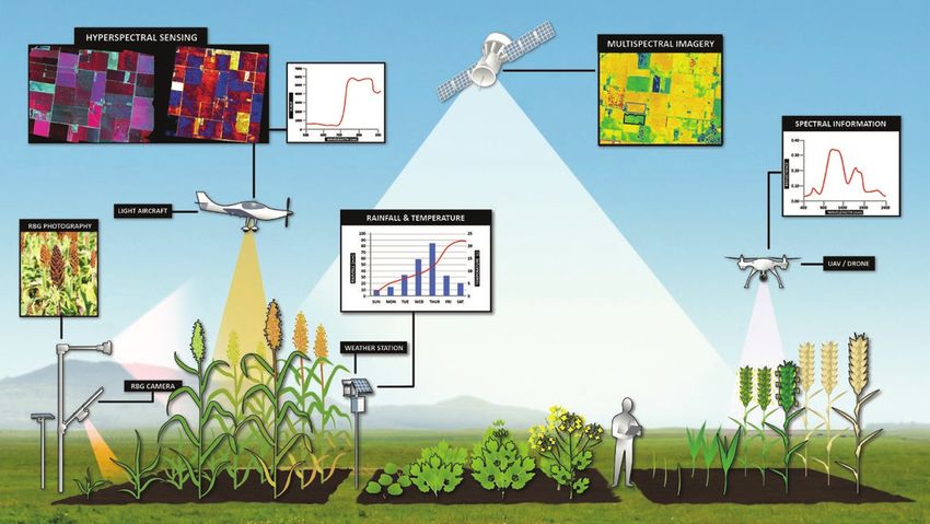
maximize efficiency of crop inputs and increase crop yields. Detecting desiccation). These practices are dependent on reliable determination
crop phenological stages at subfield and across field scales gives criti- of crop development and are not only maturity-specific but also crop
cal information that a producer can use to adjust tactical decision, species-specific. Thus, accurately predicting crop phenological stage
such as in-field inputs of nitrogen, herbicides and/or fungicides as and crop type is needed to help producers make more informed deci-
well as other management practices (e.g. salvaging crops, pre-harvest sions on variable rate application within and between fields on a farm.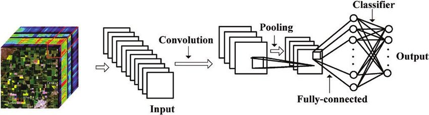
4    •   Potgieter et al.

This will lead to large cost savings and increase on-farm profitability.     development (Potgieter et al. 2011, 2013). In the Australian grain crop-
Other applications include assisting crop forecasters and managers to        ping environment, temporal information is essential for operations
monitor large cropping areas where crop phenology could be matched           such as disease and weed control (where different chemical controls
with climatic data to determine the severity and distribution of yield       are specified as suited to different crop growth stages) and the sequen-
losses to singular or additive effects of events such as frost, heat and     tial decisions of application of nitrogen (N) fertilizer in cereals in the
crop stress. In addition, by having specific estimates of crop type and      period between mid-tillering and flowering. Globally, current systems
phenology will accurately capture the interactions between G × E × M         such as the ‘Monitoring Agriculture Remote Sensing’ crop monitor-
at a subfield level and thus increase the accuracy of crop production        ing for Europe, ‘CropWatch’ from China as well as the USDA system
estimates when aggregated to a regional scale (McGrath and Lobell            mainly use MODIS and estimates are available after crop emergence
2013). We discuss in detail the digital technologies that are available      with moderate accuracies (Delincé 2017b). Recently, a study using

                                                                                                                                                                 Downloaded from https://academic.oup.com/insilicoplants/article/3/1/diab017/6279904 by guest on 22 September 2021
to predict crop type and crop phenology.                                     Sentinel-2 applying supervised crop classification, across Ukraine
                                                                             and South Africa, showed reasonable overall accuracy (>90%) but
                                                                             less discriminative power in specific crop types (>65%) (Defourny
    1.2 Crop reconnaissance from earth observation                           et al. 2019). Using time series of Landsat 8 for cropland classifications
                      platforms                                              showed accuracies of 79 % and 84 % for Australia and China, respec-
The advent of RS technologies from earth observation (EO) since              tively (Teluguntla et al. 2018b). Potgieter et al. (2013) showed that by
the end of 1960s, along with its repetitive and synoptic viewing             including the crop phenology attributes like green-up, peak and senes-
capabilities, has greatly improved our capability to detect crops on         cence from crop growth profiles (from MODIS at 250-m pixel level),
a large scale and even at daily or within-day time visits (Castillejo-       there were higher accuracies for crop-type discrimination, i.e. 96 %
González et al. 2009; Heupel et al. 2018). Earth observation tech-           and 89 % for wheat and barley, respectively. The ability to discriminate
nology has been applied in crop-type classification over the past            chickpea was lower but still reasonably high at 75 %. Although this
half-century. Due to its large-scale acquisition capability and regu-        exemplified the likely potential of fusing higher resolution EO with
lar intervals, it is ideal for tracking the phenological stage of a crop.    biophysical modelling, the method requires validation across regions
Many studies have tested the efficiency of using either single-date          and further innovation to determine crop type early in the season and
RS imagery (Langley et al. 2001; Saini and Ghosh 2018, 2019), or             to estimate phenological development within crop species.
multi-temporal RS imagery for crop-type identifications (McNairn                  Accurate classification of specific crop species from RS data
et al. 2002; Van Niel and McVicar 2004; Potgieter et al. 2007;               remains a challenge since cropping systems are often diverse and com-
Upadhyay et al. 2008). Multi-temporal classification approaches              plex, and the types of crops grown, and their growing season vary from
have proved more accurate in discriminating between different crop           region to region. Consequently, the success of RS approaches requires
types (Langley et al. 2001; Van Niel and McVicar 2004).                      calibration to local cropping systems and environmental conditions
    Crop monitoring approaches utilizing meteorological data and             (Nasrallah et al. 2018). Other factors that can affect the classification
EO have been developed globally to support efforts in measuring ‘hot         accuracy include (i) field size, (ii) within-field soil variability, (iii) diver-
spots’ of likely food shortages and thus assisting issues related to food    sified cropping patterns due to different varieties, (iv) mixed cropping
insecurity. However, such frameworks are tailored to meet the needs          systems with different phenological stages, (v) wide sowing windows
of different decision-makers and hence they differ in the importance         and (vi) changes in land use cropping patterns (Medhavy et al. 1993;
they place on inputs to the system as well as how they disseminate           Delincé 2017b; Zurita-Milla et al. 2017). Environmental conditions,
their results (Delincé 2017a). It is evident that crop monitoring and        such as droughts and floods, can further affect the reflectance signal
accurate yield and area forecasts are vital tools in aid of more informed    and thus reduce the classification and prediction accuracies (Allan
decision-making for agricultural businesses (e.g. seed and feed indus-       2000; Cai et al. 2019). The application of multi-date RS imagery for
try, bulk handlers) as well as government agencies like Australian           crop land use classification and growth dynamics estimates have led
Bureau of Statistics (ABS) and Australian Bureau of Agricultural and         to an ability to estimate crop growth phenological attributes, which
Resource Economics (ABARES) (Nelson 2018). However, there is a               are species-specific and often distinguishable, using time-sequential
current gap constraining the ability to accurately estimate crop phenol-     data of vegetation index profiles and harmonic analysis (Verhoef et al.
ogy and crop species at field scale. This is mainly due to the coarse res-   1996).
olution (≥30 m), and infrequent revisiting periods (≥16 days) of the              The following sections discuss the application of EO platforms to
long-term established satellite imagery utilized by current vegetation       detect and quantify crop species by fields and the crop growth dynam-
mapping systems. Newer satellites, like Sentinel and PlanetScope, have       ics, both considered at a ‘regional’ level. Specifically, we cover (i) avail-
higher spatial and temporal resolution. The massive data throughput of       able EO platforms and products for crop-related studies, (ii) analytical
these platforms create challenges and opportunities for near-real-time       approaches and sensor platforms in detecting crop phenology and
analysis.                                                                    discriminating between crop types, (iii) the application of machine
    Crop-type classification is of key importance to determine crop-         learning (ML) algorithms in the classification of crop identification
specific management in a spatial-temporal context. Detailed spectral         and growth dynamics, (iv) the role of crop modelling to augment
information provides opportunities for improving accuracy when               crop phenology estimates from RS, (v) current limitations, (vi) pro-
discriminating between different crop types (Potgieter et al. 2007),         posed framework addressing the challenges and (vii) finally potential
but multi-temporal data are required to capture crop-specific plant          implication/s to industry.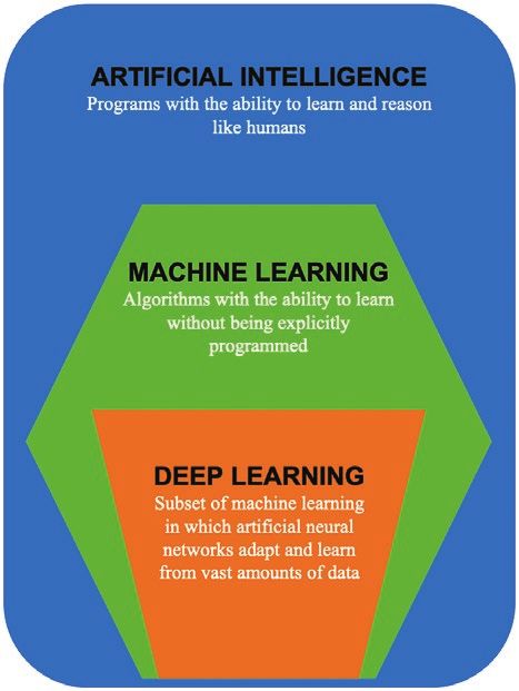
Application of digital technologies in agriculture   •   5

2. S AT E L L I T E S E N S O R S F O R V EG ETAT I O N                      at a spatial resolution of predominately 30 m. The series has enabled
             A N D C R O P DY N A M I C S                                    continuous global coverage since the early 1990s (https://landsat.gsfc.
Currently, there are >140 EO satellites in orbit, carrying sensors that      nasa.gov/). The series is still in operation with the most recent Landsat
measure different sections of the visible, infrared and microwave            8 satellite launched in 2018, which covers the same ground track
regions of the electromagnetic spectrum for the terrestrial vegetation       repeatedly every 16 days. Landsat data have served a key role in gen-
(http://ceos.org/). Figure 3 depicts a list of optical EO constellations     erating mid-resolution crop type and production prediction analysis.
currently (by 2020) in orbit and future satellite platforms planned to       For instance, the worldwide cropland maps developed in Teluguntla
be launched into space until 2039.                                           et al. (2018b) were built primarily from the Landsat satellite imagery,
    The features of these instruments depend on their purpose and            which is the highest spatial resolution of any global agriculture prod-
they vary in several aspects. This includes (i) the minimum size of          uct. At local to regional scales, the no-cost Landsat imaging has also

                                                                                                                                                         Downloaded from https://academic.oup.com/insilicoplants/article/3/1/diab017/6279904 by guest on 22 September 2021
objects distinguishable on the land surface (spatial resolution), (ii) the   been implemented for characterizing crop phenology and generating
number of electromagnetic spectrum bands sensed (spectral resolu-            detailed crop maps (Misra and Wheeler 1978; Tatsumi et al. 2015).
tion) and (iii) the intervals between imagery acquisitions (temporal         The key limitation in the use of Landsat data mainly relates to the lim-
resolution). A comprehensive understanding of these features for past,       ited data available for tracking crop growth and the difficulties in dis-
present and future sensors used for vegetation and crop detection is         criminating specific crop types (Wulder et al. 2016).
essential to develop algorithms and applications. National to regional           Although efficient land-cover classification approaches were
crop-type identification has been carried out in literatures using           developed and refined for mapping based on Landsat imagery, it was
freely available EO data, such as from Landsat, MODIS and recently           the increase in frequency of image acquisition that provided unprec-
launched Sentinel (https://sentinel.esa.int/web/sentinel/home).              edented insights about the landscape vegetation, with, e.g., MODIS.
    The first Landsat satellite was launched in 1972 and had a on-board      MODIS is currently one of the most popular multispectral imaging
multispectral scanner (MSS) for collecting land information at a land-       devices. It was first launched in 1999 by NASS and has devices record-
scape scale. Since then, Landsat has initiated a series of missions that     ing 36 spectral bands, seven (blue, green, red, two NIR bands and two
carried the enhanced thematic mapper plus (ETM+), capable of cap-            SWIR bands) of which are designed for vegetation-related studies.
turing data at eight spectral bands from visible to short-waved infrared     MODIS provides daily global coverage at spatial resolutions from 250

Figure 3. List of current (2020) and planned (up to 2039) EO satellites to target vegetation dynamics on earth (Source: http://
ceos.org).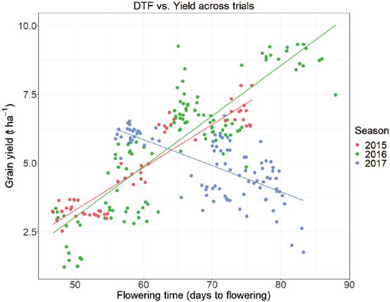
6   •   Potgieter et al.

m to 1000 km, as well as 8-day and 16-day composite vegetation indices        of its predecessors including AVHRR and MODIS (https://ladsweb.
products. Frequently acquired imageries from this sensor provide the          modaps.eosdis.nasa.gov/). The twin satellites of Sentinel-2 (A/B) with
comprehensive views of the vegetation across large areas. Analysis of         a 7-year lifetime design is also planned to be replaced in 2022–23 time
the long time series of MODIS, along with the improving understand-           frame by new identical missions taking the data record to the 2030
ing of the relations between reflectance and canopy features, makes the       time frame (Pahlevan et al. 2017).
study of vegetation dynamics on large scales possible. For instance, the
multi-year MODIS time series was implemented to characterize crop-
land phenology and to generate a global cropland extent using a global        3. D ET E R M I N I N G C R O P P I N G A R E A , C R O P
classification decision tree algorithm (Pittman et al. 2010). Similarly         T Y P E S A N D OT H E R C R O P AT T R I BU T E S
at regional scale, in Australia winter crop maps have been produced                                 FROM R S
                                                                                 3.1 Using single-date satellite imagery to derive

                                                                                                                                                            Downloaded from https://academic.oup.com/insilicoplants/article/3/1/diab017/6279904 by guest on 22 September 2021
annually using crop phenology information derived from a time series
of MODIS data (Potgieter et al. 2007, 2010). A major limitation in                       cropping area and crop types
MODIS image-based study is its relatively coarse spatial resolution           Since the early 80s, single-date imagery has been used for crop detec-
(250 m), which cannot provide information at a small scale (e.g. field        tion from RS (Macdonald 1984). Approaches based on single-date
and within field).                                                            data typically target imagery around the maximum vegetative growth
    More recently, Sentinel-2 has served as an alternative source of data     period to discriminate between all cropping areas and non-cropping
for crop researchers. Sentinel-2A was launched in 2015 and provides           land use areas (Davidson et al. 2017). In situations where cloud-free
wide-area images with resolutions of 10 m (visible and near-infrared, or      images are rare during the vegetation period, especially in regions close
NIR), 20 m (red-edge, NIR and short-wave infrared, or SWIR) and 60            to the equatorial with few clear days, single-date image approaches can
m (visible to SWIR for atmospheric applications) and a 10-day revisit         be useful (Matvienko et al. 2020). Such approaches require less time
frequency. The identical Sentinel-2B satellite was launched in 2017,          and cost (Langley et al. 2001), and receive moderate accuracy in some
which increased Sentinel-2’s revisit capacity to five days. Sentinel-2        local scale studies (Table 1).
imagery has been available free since October 2015. With the high                  Single-date imagery has been used for crop-type classification
level of spatial and temporal detail, as well as the complementarity          (Table 1). In Saini and Ghosh (2018), NIR, red, green and blue band
of the spectral bands, Sentinel-2 has enabled tracking the progressive        reflectance from a single-date Sentinel-2 (S2) imagery was adopted
growth of crops and identifying the most relevant crop-specific growth        for crop classification within a 1000 km2 region using both support
variables (e.g. crop biophysical parameters, start of season, greening up     vector machine (SVM) and random forest (RF) methods. The study
rate, etc.).                                                                  classified fields with a moderate accuracy (80 %) for wheat crops, with
    In addition, small and relatively inexpensive to build satellites         wheat pixels misclassified as fodder due to the spectral similarities. In
known as CubeSats have increased over the last decade (McCabe et al.          Matvienko et al. (2020), multispectral band reflectance from single S2
2017). These new satellites, such as Planet Labs (‘Planet’) PlanetScope       images acquired around peak greenness of crops in South Africa, along
and Skybox imaging SkySat satellites, enables the creation of a collec-       with S2 band-derived vegetation indices were input into both ML (i.e.
tion of both high spatial (
Application of digital technologies in agriculture • 7
Table 1. List of studies using single-date RS date for crop classification.
Targeted crops Sensor, temporality Algorithms Accuracy Reference
Maize, cotton, Sentinel-2B, image K-nearest-neighbours, RF0 and Gradient Best result is achieved for gradient Matvienko
grass and acquisition boosting applied to all 13 spectral bands boosting with overall accuracy et al.
other date centred on and vegetation indices (NDVI1, EVI2, of 77.4 % (2020)
intercrops 1/1/2017 near MSAVI3 and NDRE4)
peak greenness
Wheat, Sentinel-2, image RF and SVM5 methods applied to stacked RF and SVM received 84.22 % Saini and
sugarcane, acquired in the blue, green, red and NIR bands and 81.85 % overall accuracy, Ghosh
Downloaded from https://academic.oup.com/insilicoplants/article/3/1/diab017/6279904 by guest on 22 September 2021
fodder and growing season respectively (2018)
other crops
Cotton, RapidEye, acquired Softmax regression, SVM, a one-layer NN6 All algorithms did well and Rustowicz
safflower, in middle of the and a CNN7 applied to the five spectral received accuracies around (2017)
tomato, growing season bands of RapidEye 85 %
winter (mid-July)
wheat,
durum
wheat
Sunflower, QuickBird, acquired Parallelepiped, Minimum Distance, Object-based classification Castillejo-
olive, winter on 10/7/2004 Mahalanobis Classifier Distance, outperformed pixel-based González
cereal Spectral Angle Mapper and Maximum classifications. Maximum et al.
stubble and Likelihood applied to pan-sharpened likelihood received best overall (2009)
other land multispectral bands of RapidEye accuracy of 94 %.
covers
Corn, rice, WorldView-2, SVM applied to the eight spectral bands, Textures marginally increased Wan and
peanut, acquired on plus the NDVI and textures overall classification accuracy Chang
sweet 3/10/2014 to 95 % (2019)
potato, soya
bean
Rice, maize, Landsat 7, all Maximum likelihood with no probability For example, for sorghum, the Van Niel
sorghum imagery during threshold applied to all single-date primary window for identifying and
and the summer images (to determine the best the crop was from mid-April to McVicar
soybeans growing season identification window using single image May, with producer’s accuracy (2004)
were acquired for different crops) > 75 % and user’s accuracy >
60.
Corn, cotton, Spot-5 10-m image, Minimum Distance, Mahalanobis Distance, Maximum likelihood classification Yang et al.
sorghum acquired in the Maximum Likelihood, Spectral Angle with 10-m spectral bands (2011)
and middle of growing Mapper and SVM were applied to the received best overall accuracy
sugarcane season for most four original 10-m resolution band and >87 % across the sites. Increase
crops the simulated 20 m and 30 m bands (for in pixel size did not significantly
checking the impacts of pixel sizes). affect accuracy.
Soybean, ASD handheld Using discriminant function analysis to The crops can be effectively Wilson et al.
canola, spectroradiometer classify collected reflectance data into distinguished using bands in (2014)
wheat, oat groups visual and NIR bands with
and barley single-date data collected
75–79 days after planting
Maize, carrots, Sentinel-2 Used 10 m blue, green, red and NIR for Received overall accuracy 76 % for Immitzer
sunflower, segmentation and all bands (except crops; red-edge and short-wave et al.
sugar beet atmospheric) for classification using RF infrared bands are critical for (2016)
and soya algorithm vegetation mapping
(2019), the 2-m WorldView-2 multispectral and single-date data were The rich spectral information (eight spectral bands), along with NDVI
also tested for discriminating among crops including corn, paddy rice, and texture information were input into a SVM classifier that achieved
soybean and other vegetable crops in a small experiment site (53 ha). overall accuracy >94 %.8 • Potgieter et al.
Determining crop type from single-date images remains a chal- stages. Increasing redundant and temporal autocorrelated information
lenge mainly due to the complex reflectance signals within and when adding more dates to a pixel can cause overfitting of the model
between fields (Saini and Ghosh 2018). The main concept behind and reduce discrimination power (Langley et al. 2001; Van Niel and
crop classification with satellite imagery is that different crop types McVicar 2004; Zhu et al. 2017).
would present different spectral signatures. However, it is often found With the increased availability of more frequent observations, a
that different crop types exhibit similar responses at a particular phe- more efficient way of using time-series data for deriving phenologi-
nological stage. In addition, the much wider bandwidths around each cal indicators is increasingly adopted for regional crop mappings. This
centre wavelength in some satellites (e.g. Landsat), results in increased allows the creation of a time series that is representative of the crop
spectral confusion and reduced separability between crop types growth dynamics at a pixel scale. Applications of traditional time-
(Palchowdhuri et al. 2018). To address these shortcomings, two major series approaches include harmonic analysis or wavelet (Verhoef et al.
Downloaded from https://academic.oup.com/insilicoplants/article/3/1/diab017/6279904 by guest on 22 September 2021
practices have been implemented. In the first approach, the image is 1996; Sakamoto et al. 2005; Potgieter et al. 2011, 2013). This produces
segmented before an object-based classification is introduced, which crop-related derivate metrics such as start of season, the peak green-
significantly decreases salt-and-pepper noises that are commonly seen ness, and end of season and area under the curve. Crop classification
in pixel-based classification efforts (Castillejo-González et al. 2009; using these derived features are reported to have improved classifica-
Peña-Barragán et al. 2011; Li et al. 2015). In addition, incorporating tion accuracy compared to using original multi-date vegetation index
texture-based information tend to substantially improve the classifi- values (Simonneaux et al. 2008). Extraction of phenological features
cation (Puissant et al. 2005; Wan and Chang 2019). However, due to is most efficient with frequently acquired and evenly spaced RS data
different sowing dates and environments, crop phenology can differ at from across the entire crop growth period. For example, daily MODIS
any single point in time. In the second approach images are aligned observations and associated 8-day and 16-day composite products
around specific physiological (flowering) or morphological (maxi- are frequently utilized to analyse changes in crop phenology and dis-
mum canopy) stages and can improve crop separability. For example, criminate crops and vegetation types at regional and national scales
the highest overall single-date classification accuracy for summer crops (Wardlow and Egbert 2008; Wang et al. 2014). However, the method
in south-eastern Australia was established to occur late February to is sensitive to missing data and the presence of cloud/shadow pixels.
mid-March (Van Niel and McVicar (2004). By contrast, the optimal A more complex, but more robust and widely used, feature extrac-
timings to classify individual summer crop were different and may vary tion approach is based on curve fitting of the time-series vegetation
across seasons. For example, in Australian environments, sorghum index. Here, a continuous time series of the targeted vegetation index
can be distinguished from other summer crops most effectively from is generated by fitting a pre-defined function to fill in missing data due
early April until at least early May. Similarly winter cereals (including to cloud/shadow cover. A range of mathematical functions have been
wheat, barley and other winter crops in the study) presented high clas- applied to fit the time series of the vegetation index, including linear
sification accuracy from July to August in Brazil (Lira Melo de Oliveira regression (Roerink et al. 2000), logistic (Zhang et al. 2003), Gaussian
Santos et al. 2019). In North-eastern Ontario, the best acquisition time (Potgieter et al. 2013), Fourier (Roerink et al. 2000), and Savitzky-
of satellite data for separating canola, winter wheat and barley was Golary filter (Chen et al. 2004). A detailed comparison of curve fitting
~75–79 days after planting (Wilson et al. 2014). algorithms was made by (Zeng et al. 2020). These approaches have
been intensively applied to discriminate between crop types across
3.2 Using time-sequential imagery to derive crop regions. Numerous studies have demonstrated that the intra-class
attributes (between crop classes) confusion can be effectively reduced by har-
Various approaches making use of multi-date imagery have been devel- nessing the phenological similarities between crop species within the
oped to harness all the information captured from RS throughout the same geographical region (Sakamoto et al. 2005; Potgieter et al. 2013).
crop growth period (Table 2). A simple strategy for discriminating dif-
ferent crop types using multi-date imagery is to combine image data 3.3 Multispectral and hyperspectral data to detect
from various dates to form a single multi-date image prior to classifi- crop phenology and crop type from airborne
cation (Van Niel and McVicar 2004). Similar strategies directly using platforms
available RS observations (normally in terms of vegetation indices) at Recent advances in sensor technologies, which have become lighter with
different crop development stages as independent variables and input enhanced resolution (e.g. improved spectral and spatial resolutions of
into different classification algorithms for mapping crop distributions cameras and sensors, and increased accuracies of geographical position-
(dependent variable) have been widely adopted in literature (Wang ing systems (GPS)), have led to the rapid increase in the use of drones or
et al. 2014). The direct use of original vegetation index values works unmanned aerial vehicles/aerial systems/remotely piloted aircraft system
well in studies with clear observations at multiple periods, especially (known as UAV, UAS and RPAS). Unmanned aerial vehicles allow high-
during key growth stages (e.g. around flowering and peak greenness). throughput phenotyping of targeted traits like head number, stay-green,
However, in these studies the sequential relationships of multi-date biomass and leaf area index (LAI) with specifically developed predictive
values were ignored and therefore their relationships to specific crop models (Chapman et al. 2014, 2018; Potgieter et al. 2017; Guo et al. 2018).
growth stages are not considered. Stacking multi-date images into The use of UAVs in land cover detection has shown promise
one for classification works most effectively when only limited satel- (Table 3). Images captured with different sensors/cameras includ-
lite observations are available, including observations for key growing ing RGB, multispectral, hyperspectral and thermal cameras haveApplication of digital technologies in agriculture • 9
Table 2. List of studies using a time-sequential data approach for crop classification.
Targeted crops Sensor, temporality Algorithms Accuracy Reference
Corn, soybean, 500-m, 8-day MODIS SVM applied to the NDVI time Overall accuracy >87 % across three Wang et al.
spring series of different crops directly consecutive seasons (2014)
wheat and
winter
wheat cross
seasons
Winter wheat, Landsat 7/8, Using fuzzy c-means clustering Good overall accuracy in 2015 (89 %) Heupel et al.
Downloaded from https://academic.oup.com/insilicoplants/article/3/1/diab017/6279904 by guest on 22 September 2021
barley, rye, Sentinel-2A and progressively cluster the fields into but low accuracy (77 %) in 2016 due (2018)
rapeseed, RapidEye fused groups and then assign the groups to unfavourable weather
corn and NDVI series for with classes based on expert
other crops two crop seasons experience
Corn and Landsat TM and RF algorithm applied to different Different combination of indices received Zhong et al.
soybean ETM+; using band combination of multi-temporal overall accuracy higher than 88 % (2014)
crops reflectance and EVI-derived transitional dates, the when using data collected in the same
during calculated EVI from band reflectance at the transitional year. Using phenological variables
multiple all available imagery dates and accumulated heat only and applying to different years
years in each year (growing degree day) received accuracy >80 %.
Corn, soybean Landsat TM available Two data sets fused (using Overall accuracy 90.87 %; object-based Li et al.
and winter scenes across ESTARFM) to create an enhanced segmentation and then classification (2015)
wheat the season and time series; decision tree method reduced in-field heterogeneity and
8-day NDVI from using time-series indices derived spectral variation and increased
MODIS (500 m) from fitted NDVI profiles accuracy
Rice HJ-1A/B and MODIS ESTARFM fused time series to Received overall accuracy of 93 %. Singha et al.
derive phenological variables and While the detection at large regions (2016)
was used for constructing decision underestimated rice areas by 34.53 %
trees for rice fields compared to national statistics.
Rice (single-/ 8-day, 500-m MODIS Based on the cubic spline-smoothed The overall accuracy was >80.6 % across Son et al.
double-/ surface reflectance EVI profile, the regional peak and the studied period. While the method (2014)
triple- product from 2000 time of peak were identified to overestimated rice area from 1 to 16 %
cropped to 2012 determine single/double/triple when compares to statistics over the
rice) rice fields period.
Barley, wheat, One WorldView -3 Tested RF on three vegetation Using RF alone received overall accuracy Palchowdhuri
oat, oilseed, and two Sentinel-2 indices (NDVI, GNDVI, SAVI). of 81 %, and introducing the decision et al.
maize, peas images acquired And then introduced decision tree modeller increased the accuracy (2018)
and field during the major tree to improve the result by using to 91 %
beans vegetative stage S2 bands to separate spectrally
overlapping crops.
Wheat, maize, Available Sentinel-2 Time-weighted dynamic time Object-based TWDTW performed best Belgiu and
rice and images warping (TWDTW) analysis and received overall accuracy from Csillik
more to the Sentinel-2 NDVI series, 78 to 96 % across three diversified (2018)
and results are compared to RF regions. Region has higher complex
outputs. temporal patterns showed relative
lower accuracy
cereals, canola, All dual-polarized Defined six phenological stages for The phenological sequence pattern- Bargiel
potato, Sentinel-1 images each crop and classify the crops based classification received overall (2017)
sugar beet, covering the two according to their phenological better results than RF and maximum
and maize crop seasons sequence patterns. likelihood; and it is resilient to
across two phenological differences due to
seasons farming management10 • Potgieter et al.
Table 3. List of studies using UAV platform collected data for crop classification.
Targeted crops Sensors Algorithm Accuracy Reference
Maize, sugar beet, Canon RGB and Canon RF applied to the texture Best pixel-based overall accuracy Bohler
winter wheat, NIRGB information extracted from is 66 %, and best object-based et al.
barley and photos accuracy is 86 % (2018)
rapeseed
Cabbage and Multi-date Canon camera RF and SVM applied to multi- Multi-date photos received high Kwak and
potato with NIR, red and data or single-date photo’s accuracy (>98 %) and texture Park
green bands bands and extracted texture contribute few; single-date photos (2019)
Downloaded from https://academic.oup.com/insilicoplants/article/3/1/diab017/6279904 by guest on 22 September 2021
received accuracy around 90 % with
significant benefit from texture.
Cultivated fields Single-date RGB camera Hierarchical classification Overall accuracy is 86.4 % Xu et al.
(aggregated based on vegetation index (2019)
crops) and texture
Wheat, barley, Multi-date photos with Decision tree applied to the Overall accuracy > 99 % in Latif
oat, clover and green, red and NIR derived NDVI series recognizing 17 crops; and early- to (2019)
other 13 crops bands mid-season photos contribute more
to classification
Corn, wheat, Single-date RGB and Object-based image Multispectral data received higher Ahmed
soybean, alfalfa multispectral (G, R, classification method accuracy (89 %) than RGB photos et al.
NIR and red-edge) implemented and classes (83 %) (2017)
were assigned based on
their spectral characteristics
Cotton, rape, One-date hyperspectral Proposed a Spectral-spatial SSF-CRF outperformed other Wei et al.
cabbage, image containing 270 fusion based on conditional classifiers, e.g. RF and received (2019)
lettuce, carrots spectral bands random fields method overall accuracy > 98 % at the test
and other land (SSF-CRF) sites (400 × 400 pixels in site 1 and
covers 300 × 600 pixels in site 2)
Cowpea, soybean, Hyperspectral image SSF-CRF SSF-CRF method received overall Zhao
sorghum, containing 224 bands accuracy 99 % at site 1 (400 × 400 et al.
strawberry, at resolution of 3.7 m pixels), and 88 % at site 2 (303 × (2020)
and other land (site 1) and image with 1217 pixels)
covers 274 channels at 0.1 m
been used to monitor crop type, crop canopy and to quantify can- The rich spectral information captured from recently developed
opy structural and biophysical parameters (LAI, photosynthetic and UAV-borne hyperspectral sensors is an attractive option for detect-
non-photosynthetic pigments, transpiration rates, solar-induced flu- ing crop species. Wei et al. (2019) proposed a ‘Spatial-Spectral Fusion
orescence) (Ahmed et al. 2017; Bohler et al. 2018). Analysis of mul- based on Conditional Random Fields’ (SSF-CRF) classification
tispectral (NIR, red, green and blue) and multi-date data on-board method for harnessing hyperspectral data in classifying crop types.
UAVs have enabled the classification between cabbage and potato This included deriving the morphology, spatial texture, and mixed
crops (overall accuracy > 98 %) (Kwak and Park 2019). It was also pixel decomposition using a CRF mathematical function for each
found that using single-date UAV data is less efficient in discrimi- spectral band. This resulted in creating a spectral-spatial feature vec-
nating different crops due to the heterogeneity captured by the fine tor to enhance the spectral changes and heterogeneity within the same
resolution pixels. However, the inclusion of additional texture infor- feature. Applying the method in two experimental sites (~400 × 400
mation (e.g. homogeneity, dissimilarity, entropy and angular second pixels area) achieved accuracy >97 %, primarily for vegetable crops.
moment) in classifying single-date UAV images could significantly Furthermore, out-scaling such an approach allowed distinction
increase the classification accuracy (Kwak and Park 2019; Xu et al. between various crop types (soybean, sorghum, strawberry and other
2019). The use of data from optical cameras sensitive to the visible land cover types) in larger fields (over 300 × 1200 pixels) and other
region (RGB) also had reasonable success in crop-type detection. regions in Hubei province of China, with an overall accuracy of 88 %
For example, a multi-date NDVI decision tree classifier had a high (Zhao et al. 2020).
overall accuracy (99 %) in discrimination 17 different crops in an Although, airborne platforms are capable of capturing high spatial
agronomy research at plot scale (Latif 2019). (Application of digital technologies in agriculture • 11
classification accuracies as achieved using single index at lower (e.g. >1 superior accuracy (overall > 88 %) compared to using each of the indi-
m) resolution across multiple dates (Gamon et al. 2019). For example, vidual data sets separately (Zhao et al. 2019).
Bohler et al. (2018) compared the change in accuracies for resampled
data captured on-board UAV into different spatial resolution (from 0.2 4. L A N D U S E A N D C R O P C L A S S I F I C AT I O N
to 2 m) and found that the best resolution for discriminating individ- A P P R OA C H E S
ual crops was around 0.5 m. This was mainly due to the heterogeneous Various statistical approaches are frequently utilized to classify RS data
landscape, which resulted in smaller pixel sizes resulting in a decrease into different land use or crop-type categories. Such approaches can
of classification accuracies. Thus, having higher resolution can be a be divided into supervised, unsupervised or decision tree classifica-
disadvantage due to the increase of mixed reflectances from more tion approaches (Campbell 2002). These are usually applied on either
prominent features, such as soil background, single leaves, shadows the entire time series or a derivative of the time series representing
Downloaded from https://academic.oup.com/insilicoplants/article/3/1/diab017/6279904 by guest on 22 September 2021
from leave. Nevertheless, it is generally accepted that high-resolution the main aspects of crop growth. However, the advance in comput-
hyperspectral imagery opens new opportunities for the independent ing power, e.g. cloud computing and high-resolution imagery, has also
analysis of individual scene components to properly understand their allowed the application of ML and more complex deep learning (DL)
spectral mixing in heterogeneous crops. approaches.
It is anticipated that the ability of capturing high temporal, spatial
and spectral resolution reflectance data on board of UAVs will enable 4.1 Unsupervised and supervised approaches
further advancements in understanding of physiological and func- Unsupervised classification algorithms, e.g. ISODATA and K-means
tional crop processes at the canopy level. clustering, define natural groupings of the spectral properties at pixel
scales and requires no prior knowledge (Xavier et al. 2006). These
3.4 Integrating crop information derived from dif- approaches will attempt to determine a number of groups and assign
ferent RS platforms pixels to groups with no input from users. In contrast, decision tree
Remote sensing-derived information has four attributes: (i) spatial approaches need to have specific threshold cut-offs that allows for
resolution, (ii) temporal resolution, (iii) number of spectral bands crop-type discrimination (Lira Melo de Oliveira Santos et al. 2019). In
and (iv) the band or wavelength width of each band. Currently, a few unsupervised classifications, the number of classes are usually arbitrar-
attempts have been made to integrate information from different sens- ily defined making it a less robust approach than supervised classifica-
ing platforms mainly through fusion approaches. Fusion happens by tion (Niel and McVicar 2004; Xavier et al. 2006).
incorporating such metrics from two different RS platforms utilizing Up to now, most crop classification studies have extensively used
RF classifier to discriminate crop type and other land use classes (Lobo supervised classification methods, i.e. data sets are split (75:25) and
et al. 1996; Ban 2003; McNairn et al. 2009; Ghazaryan et al. 2018; Lira there is some kind of ‘training’ step, followed by a ‘validation’ step on
Melo de Oliveira Santos et al. 2019; Zhang et al. 2019). A large portion different samples of the data set. To come to a final model, expertise in
of the approaches have used derived RS variables (indices) that highly designing and setting parameters for the algorithms becomes a part of
correlate with known crop morphological and physiological attributes the input. These include maximum likelihood (MLC), SVMs and RF.
(e.g. LAI, percent cover, green/red chlorophyll, canopy structure or The common principle behind these supervised classifiers is that the
canopy height). classifier is trained on field observations (prior knowledge) and then
Furthermore, some studies generate a continues time series of the model is applied to the remainder of imagery pixels either for a few
enhanced EO data through the integration of RS data that varies imageries or across all dates.
both spatially as well as temporally (e.g. MODIS 25 m and Landsat The MLC is one of the most traditional parametric classifiers and is
30 m) (Liu et al. 2014; Li et al. 2015; Sadeh et al. 2020; Waldhoff et al. usually used when data sets are large enough so that the distributions
2017). Such an approach is known as the spatial-temporal adaptive of objects can be assumed approaching Gaussian normal distribution
reflectance fusion model (STARFM). This model was developed by (Benediktsson et al. 1990; Foody et al. 1992). Briefly, MLC assigns
Feng et al. (2006) to first fuse Landsat and MODIS surface reflec- each pixel to a class with the highest probability using variance and
tance over time (Li et al. 2015; Zhu et al. 2017). Applying STARFM covariance matrices derived from training data (Erbek et al. 2004).
to generate missing dates of high-resolution imagery can significantly Studies have found that MLC could work effectively with relative low
decreased the average overall classification errors when compared to dimensional data and could achieve comparatively fast and robust clas-
classification using Landsat data only (Zhu et al. 2017). However, sification results when fed with sufficient quality data (Waldhoff et al.
care should be taken when using such an approach where there is a 2017).
high frequency of missing data, since it can result in high prediction SVM is a non-parametric classifier, which makes no assumptions
errors (Zhu et al. 2017). of the distribution type on the training data (Foody and Mathur 2004;
Efforts have also attempted to fuse high-resolution UAV images Ghazaryan et al. 2018). Its power lies in the fact that it can work well
(with limited spectral bands) with multispectral satellite images with higher dimensional features and generalize well even with a small
(higher number of spectral bands but with relatively lower spatial reso- number of training samples (Foody and Mathur 2004; Mountrakis
lution) for finer crop classifications ( Jenerowicz and Woroszkiewicz et al. 2011).
2016; Zhao et al. 2019). Fusion of Sentinel-2 imagery with UAV Currently, one of the most commonly used approaches is RF,
images through a Gram-Schmidt transformation function resulted in especially for crop discrimination. RF is an ensemble machine12 • Potgieter et al.
learning classifier that aggregates a large number of random deci-
sion trees for classification (Breiman 2001). RF can efficiently
manage large data sets with thousands of input variables and is
more robust in accounting for outliers (Breiman 2001; Li et al.
2015). In addition, RF does not result in overfitting when increas-
ing the number of trees (Ghazaryan et al. 2018). A recent study
using a time series of Landsat and Sentinel with a supervised RF
two-step approach resulted in moderately acceptable accuracies
(>80 %) to discriminate crops from non-crops across the broad
land use of China and Australia (Teluguntla et al. 2018a). The com-
Downloaded from https://academic.oup.com/insilicoplants/article/3/1/diab017/6279904 by guest on 22 September 2021
prehensive list of supervised classifiers and their comparisons is
available in the review from Lu and Weng (2007). Overall, there is
no single best image classification method for detailed crop map-
ping. Methodologies based on supervised classifiers generally out-
perform others (Davidson et al. 2017), but require training with
ground-based data. SVM, MLC and RF supervised classifiers are
also grouped within the suite of first-order ML approaches.
Supervised classification remains the standard approach when
higher classification accuracies are needed. However, it requires good
quality and a significant high sample of local field observation data for
developing the training classifier. This leads to challenges for specific
crop-type classification in regions where spatially explicit field level
information is unavailable.
Figure 4. The relationship of AI, ML and DL (Adapted from
www.argility.com).
4.2 ML and DL techniques
Both ML and DL approaches are subsets of artificial intelligence
(AI) techniques (Fig. 4). Machine learning builds models based on For example, Hu et al. (2015) developed a 1D CNN architecture
the real-world data and the object it needs to predict. Artificial intel- containing five layers with weights for supervised hyperspectral image
ligence techniques are typically trained on more and more data over classification for eight different crop types in India, which generated
time, which improves the model parameters and increases prediction better results than the classical SVM classifiers. A 2D convolution
accuracy. Machine learning approaches includes supervised learning, within the spatial domain in general can discriminate crop classes
unsupervised learning and reinforcement learning techniques. Deep more reliably than 1D CNNs (Kussul et al. 2017). One recent study
learning extends classical ML by introducing more ‘depth’ (complex- also developed 3D CNN architectures to characterize the structure
ity) and transforming data across multiple layers of abstraction using of multispectral multi-temporal RS data ( Ji et al. 2018). In this study,
different functions to allow data representation hierarchically. the proposed 3D CNN framework performed well in training 3D
Deep learning techniques have increasingly been used in RS appli- crop samples and learning spatio-temporal discriminative representa-
cations due to their mathematical robustness that generally allows more tions. Jin et al. (2018) concluded that 3D CNN is especially suitable
accurate extraction of features within large data sets. Artificial neural for characterizing the dynamics of crop growth and outperformed 2D
networks (ANN), recurrent neural networks (RNNs) and convolu- CNNs and other conventional methods ( Ji et al. 2018).
tional neural networks (CNNs) represent three major architectures of Recurrent neural network is another well-adopted DL archi-
deep networks. ANN is also known as a Feed-Forward Neural network tecture for classification. As indicated by its name, RNNs are
because the information is processed only in the forward direction. specialized for sequential data analysis and have been considered
Limited by its design, it cannot handle sequential or spatial information as a natural candidate to learn the temporal relationship in time-
efficiently. Traditionally, a CNN consists of a number of convolutional series image. In Ndikumana et al. (2018), two RNN-based clas-
and subsampling layers optionally followed by fully connected layers. It sifiers were implemented to multi-temporal Sentinel-1 data over
is designed to automatically and adaptively learn spatial hierarchies of an area in France for rice classification and received notable high
features. Due to the benefit of its architecture, it has become dominant accuracy (F-measure metric of 96 %), thus outperforming classical
in various computer vision tasks (Yamashita et al. 2018). In agriculture approaches such as RF and SVM. However, in Zhong et al. (2019),
applications, CNN can extract distinguishable features of different the RNN framework applied to Landsat EVI time series received
crops from remotely sensed imagery in a hierarchical way to classify lower crop classification accuracy (82 %) than results with a 1D
crop types. The term ‘hierarchical’ indicates the convolution process CNN framework (86 %), which considered the temporal profiles
through either 1D across the spectral dimension, 2D across the spatial as spectral sequences.
dimensions (x/y locations), or 3D across the spectral and the spatial Overall, NNs have the properties of parallel processing ability, adap-
dimensions simultaneously (Zhong et al. 2019). Figure 5 depicts the tive capability for multispectral images, good generalization, and not
broad architecture of convolution and image classification steps. requiring any prior knowledge of the probability distribution of theYou can also read