RESEQ SIMULATES REALISTIC ILLUMINA HIGH-THROUGHPUT SEQUENCING DATA
←
→
Page content transcription
If your browser does not render page correctly, please read the page content below
Schmeing and Robinson Genome Biology       (2021) 22:67
https://doi.org/10.1186/s13059-021-02265-7

 METHOD                                                                                                                                              Open Access

ReSeq simulates realistic Illumina
high-throughput sequencing data
Stephan Schmeing1,2*                      and Mark D. Robinson1,2*

*Correspondence:
stephan.schmeing@uzh.ch;                      Abstract
mark.robinson@mls.uzh.ch                      In high-throughput sequencing data, performance comparisons between
1
  Institute of Molecular Life Sciences,
University of Zurich,                         computational tools are essential for making informed decisions at each step of a
Winterthurerstrasse 190, 8057                 project. Simulations are a critical part of method comparisons, but for standard Illumina
Zurich, Switzerland
2
  SIB Swiss Institute of
                                              sequencing of genomic DNA, they are often oversimplified, which leads to optimistic
Bioinformatics, Winterthurerstrasse           results for most tools. ReSeq improves the authenticity of synthetic data by extracting
190, 8057 Zurich, Switzerland                 and reproducing key components from real data. Major advancements are the inclusion
                                              of systematic errors, a fragment-based coverage model and sampling-matrix estimates
                                              based on two-dimensional margins. These improvements lead to more faithful
                                              performance evaluations. ReSeq is available at https://github.com/schmeing/ReSeq.
                                              Keywords: Simulation, Genomic, High-throughput sequencing, Illumina

                                            Background
                                            High-throughput sequencing has revolutionized biology and medicine since it allows a
                                            myriad of applications, such as studying entire genomes at base-pair resolution. The accu-
                                            racy of the obtained results after applying computational methods heavily depends on
                                            collected data and the tools used to process it. This paper focuses on standard Illumina
                                            short-read sequencing of genomic DNA (gDNA) and its BGI counterpart [1, 2], which
                                            are both obtainable for almost every molecular biology lab. In order to fully capitalize on
                                            these datasets, it is important to know the best tools for a given task, the typical error
                                            modes of these tools, and whether a result is robust to fluctuations in the data or changes
                                            in the analysis.
                                              With the ever-growing number of computational tools, evaluating their performance
                                            across the various situations in which they are applied has become an essential part of
                                            bioinformatics [3, 4]. There are two fundamental ways of doing benchmarks and valida-
                                            tions. On the one hand, results can be compared to an estimated “gold-standard” ground
                                            truth derived from real data, which can be based on consensus or an independent dataset
                                            (e.g., technology). On the other hand, tools can be compared on synthetic data, which

                                            © The Author(s). 2021 Open Access This article is licensed under a Creative Commons Attribution 4.0 International License,
                                            which permits use, sharing, adaptation, distribution and reproduction in any medium or format, as long as you give appropriate
                                            credit to the original author(s) and the source, provide a link to the Creative Commons licence, and indicate if changes were
                                            made. The images or other third party material in this article are included in the article’s Creative Commons licence, unless
                                            indicated otherwise in a credit line to the material. If material is not included in the article’s Creative Commons licence and your
                                            intended use is not permitted by statutory regulation or exceeds the permitted use, you will need to obtain permission directly
                                            from the copyright holder. To view a copy of this licence, visit http://creativecommons.org/licenses/by/4.0/. The Creative
                                            Commons Public Domain Dedication waiver (http://creativecommons.org/publicdomain/zero/1.0/) applies to the data made
                                            available in this article, unless otherwise stated in a credit line to the data.
Schmeing and Robinson Genome Biology (2021) 22:67 Page 2 of 37
are simulated from a specified ground truth that defines the desired results. Both strate-
gies can introduce biases, through deriving the ground truth or by failing to mimic the
properties of real data, respectively. Ideally, a mix of assessments from real and synthetic
data is used, where differences in the results can highlight biases and provide estimates of
uncertainty.
On real data, performance evaluations require a ground truth and estimating it with
methods similar or identical to evaluated methods can induce a bias. To reduce such
a bias, evaluations often only take into account situations where a confident consensus
can be determined or where an alternative technology delivers reliable results [5]. This
limitation necessarily reduces the breadth of method comparisons. Sometimes, these
shortcomings can be mitigated with deeper sequencing, by using multiple alternative
technologies and by carefully selecting the set of methods that go into the estimation. For
example, extensive effort went into generating datasets with ground truth to assess variant
calling on human gDNA datasets [6], such as the Genome in a Bottle Consortium [7, 8]
and Platinum Genomes [9]. Their detailed variant truth sets were derived using a consen-
sus from multiple aligner/variant caller combinations. Having multiple technologies or
pedigree information further increases the confidence in their ground truth calls. Alter-
natively, as an example of consensus-free approaches, Li et al. used Pacific Biosciences
SMRT sequencing (PacBio) to create two independent assemblies, each of a homozygous
human cell line. The combined assemblies provide the ground truth for a synthetic diploid
dataset [10]. The advantage is that no variant callers are used to estimate the truth, while
the disadvantage is that PacBio-specific errors remain. Despite the effort that went into
the three mentioned truth sets, their results do not agree on variant caller performance,
neither by value (e.g., false-positive rates of single-nucleotide polymorphisms) nor by rank
[10]. Due to an abundance of truth sets in this field, the uncertainty in the comparisons
can at least be assessed with real data alone. In other areas of research, often no published
datasets with an estimated ground truth are readily available. For example, assessing
the influence of polyploidy on variant calls using real data is limited to concordance
checks [11].
Simulated data are a cheap and orthogonal way to benchmark computational meth-
ods and can readily address the shortcomings of real data based evaluations (e.g., biases
toward certain tools or against certain genomic regions). Additionally, robustness toward
properties of data (e.g., error rates) can be easily assessed. However, accurate method
assessments require that simulated data recapitulate the important features of real data
and do not oversimplify or bias the challenge for tested methods. Despite many published
simulators, research comparing simulations has so far neglected to test for these impor-
tant features. Reviews include Escalona et al. [12], which did not show any benchmarks,
and Alosaimi et al. [13], which based the performance report on sensitivity and precision
of mapping (of simulated reads). Unfortunately, this metric says little about the quality of
the simulation; for example, a simulator that samples from unique regions of the refer-
ence and does not include any errors would receive a perfect score. A proper benchmark
requires in-depth testing across a range of use-cases, since the most important features to
mimic from real data depend on the application. We assess here many aspects of real data
and in particular whether the key features for assembly have been reproduced. Further-
more, we show using the example of mapping how to evaluate the scope of simulations in
a benchmark.Schmeing and Robinson Genome Biology (2021) 22:67 Page 3 of 37
For Illumina gDNA datasets, the simulation frameworks ART [14], pIRS [15], and
NEAT [16] represent the state-of-the-art. Additionally, BEAR [17] was included to eval-
uate the effect of their design choices that simplify metagenomic simulations. We show
below that all current simulators do an unsatisfactory job of reproducing, e.g., the k-mer
spectrum of real data, due to their incomplete models for coverage, quality, and base call-
ing. As a result, methods tested on simulated data score nearly perfectly [18], which has
presumably encouraged the field to rely on real data alone for evaluations; for example,
the Assemblathon 1 [19] used simulations, while GAGE [20] and Assemblathon 2 [21] in
the following years used real data alone.
Table 1 lists the features and input for each of the simulators compared in this study.
The two main simulation components are the coverage model and the quality and base-
call model. Coverage in ART and BEAR is modelled uniformly, while pIRS and NEAT
introduce a GC bias by comparing the coverage across the binned reference [22, 23]. This
procedure is close to the Loess model described by Benjamini and Speed [24], who show
that their alternative model based on the GC of individual fragments results in superior
predictions. Furthermore, the bias from the sequences flanking the start and end of frag-
ments [25] are not taken into account by any simulator. Finally, ART, pIRS, and BEAR
draw DNA fragment lengths from a user-defined Gaussian distribution, while NEAT uses
the empirical distribution from the input bam file.
For the qualities and base-calls, ART draws from empirical distributions of position-
dependent qualities and introduces substitution errors [26–28] according to the proba-
bility given by the quality values. InDels are inserted based on four user-specified rates
for insertion/deletion in the first/second read. In contrast, pIRS, NEAT, and BEAR draw
quality values from a non-homogeneous Markov chain, where the quality depends on the
last quality and the position in the read. pIRS then chooses a base call from a learned dis-
tribution depending on the quality, position, and reference base, while the inserted InDels
depend only on the position in the read. NEAT instead follows a decision tree, where the
occurrences of errors (substitution and InDels) only depends on the quality and the sub-
stituted nucleotide only on the reference base, while the length and nucleotides of InDels
Table 1 Overview of modelled features for the compared simulators
ART pIRS NEAT BEAR ReSeq
Coverage Parameters Parameters Parameters Parameters Mapped reads/
Parameters
GC bias – Mapped reads Mapped reads – Mapped reads
Flanking bias – – – – Mapped reads
Fragment length Parameters Parameters Mapped reads Parameters Mapped reads
Reference- – – – Hard-coded/(Reads) Mapped reads
sequence
bias
Base qualities Reads Mapped reads Reads Reads Mapped reads
Sequence – – - – Mapped reads
qualities
Substitution Hard-coded Mapped reads Hard-coded Reads Mapped reads
errors
Systematic errors – – – – Mapped reads
InDel errors Parameters Mapped reads Hard-coded Reads Mapped reads
Variants – Two genomes Vcf – Vcf
Parameters: Manually selected parameters. Reads: Learned from raw reads. Mapped reads: Learned from mapped reads.
Hard-coded: Cannot be changed. BEAR’s reference-sequence bias estimation from reads is design for metagenomicsSchmeing and Robinson Genome Biology (2021) 22:67 Page 4 of 37
have constant probabilities. It is worth mentioning that in the current version of NEAT,
only qualities can be trained, but the base-call and InDel distributions rely on pretrained
values. Specifically for metagenomics, BEAR’s error model is learned from duplicated
reads using DRISEE [29] and therefore does not require a reference. Its parameters are
obtained from exponential regression on the substitution rates by nucleotide and position
and on the InDel rates by position. A peculiar design choice of BEAR is to replace qual-
ity values at error positions with qualities generated by the error model instead of simply
having error rates depend on the quality values. Notably, neither systematic, sequence-
specific errors [30, 31] nor the relationship between quality and fragment length [32] are
included by any simulator.
The ability for users to train simulators on real data is another important feature,
because profiles require constant updates to changes in sequencers, chemistries, etc.,
and even without technology changes, developer-provided profiles are not always accu-
rate for a given use case due to differences in genome contexts or fragmentation method
(see Results). None of the simulators mentioned can be fully trained on real data, instead
relying at least partially on user-provided parameters or hard-coded models (Table 1).
Real Sequence Reproducer provides well-tested functionality to estimate the necessary
parameters from real data mapped to a reference. Based on these estimates, it produces
synthetic data with a k-mer spectrum matching real data without ever directly using k-
mer information (see below). Requiring a reference is not a big constraint, since one is
needed for the simulation anyways and furthermore, with a modest penalty in accuracy,
the ReSeq parameters can be estimated from a de novo assembly generated from the
reads.
We show that ReSeq outperforms all competitors in terms of delivering a realistic sim-
ulation and therefore lays the methodological groundwork for accurate benchmarking of
genomics tools.
Results
ReSeq consists of three parts: statistics calculation, probability estimation, and simula-
tion (Fig. 1). Statistics calculation extracts the necessary information from the mapped
reads and the corresponding reference. Afterwards, probability estimation combines
the extracted matrices into distributions. Finally, the simulation step draws from those
distributions.
For the statistics calculation, a file with variants can be specified, such that their posi-
tions in the reference are excluded from the statistics. Adapters can optionally be specified
and are automatically detected otherwise.
The simulation produces synthetic data matching the calculated statistics and estimated
biases. The reference provided can but does not need to be the same as the one used dur-
ing the statistics calculation. To impose a clear separation, we will refer to the reference
we simulate from as the template. To simulate single-end reads, the second read file can
simply be ignored; however, paired-end Illumina data are still required for the statistics
calculation. To properly handle coverage variations for sex chromosomes, mitochondria,
or metagenomics, the simulation optionally takes a reference-bias file (not necessary
if template and reference are identical). To simulate diploid and polyploid genomes or
pooled sequencing, variants can be specified. To simulate bisulfite sequencing, allele-
specific methylation values can be defined in an extended bed graph format with multipleSchmeing and Robinson Genome Biology (2021) 22:67 Page 5 of 37
Fig. 1 ReSeq overview. The three parts of ReSeq (solid, blue) with its mandatory (solid, red) and optional
(dotted, green) inputs. The italic entries for the statistics matrices are independent dimensions in the matrix,
while the normal entries are reduced to two-dimensional interactions
score columns. However, we focus here on monoploid and diploid genomes and will
not include simulations of bisulfite sequencing. For comparisons, we use ten represen-
tative datasets from different species, different Illumina machines and different adapters
(Table 2). Additionally, we included a dataset from BGI [1, 2] to investigate whether
Illumina simulators can also handle this related technology.
Generating qualities and base calls
To simulate quality values and base calls, ReSeq fills six matrices during the statistics cal-
culation (Fig. 1): insertions and deletions, systematic error rates at each reference position,
systematic error tendencies at each reference position, sequence qualities, base qualities,
and base calls. The matrices are used to query the probability of the variable of inter-
est conditional on all other variables in the matrix. For example, in a matrix containingSchmeing and Robinson Genome Biology (2021) 22:67 Page 6 of 37
Table 2 Used datasets
Identifier Sequencer Adapter Species Reference Accession ID
Sample ID
Ec-Hi2000-TruSeq HiSeq 2000 TruSeq Escherichia ASM584v2 SRR490124
coli
Ec-Hi2500-TruSeq HiSeq 2500 TruSeq Escherichia ASM584v2 SRR3191692
coli
Ec-Hi4000-Nextera HiSeq 4000 Nextera Escherichia ASM584v2 Ecoli1_L001
coli
Bc-Hi4000-Nextera HiSeq 4000 Nextera Bacillus ASM782v1 Bcereus1_L001
cereus
Rs-Hi4000-Nextera HiSeq 4000 Nextera Rhodobacter ASM1290v2 Rsphaeroides1_L001
sphaeroides
At-HiX-TruSeq HiSeq X Ten TruSeq Arabidopsis TAIR9.171 ERR2017816
(unknown thaliana
barcode)
Mm-HiX-Unknown HiSeq X Ten Unknown Mus GRCm38.p6 ERR3085830
muscu-
lus
Hs-HiX-TruSeq HiSeq X Ten TruSeq Homo GRCh38.p13 ERR1955542
sapiens
Hs-Nova-TruSeq NovaSeq 6000 TruSeq Homo GRCh38.p13 PRJEB33197
sapiens
Ec-Mi-TruSeq MiSeq TruSeq Escherichia ASM584v2 DRR058060
coli
At-BGI BGISEQ-500 BGISEQ Arabidopsis TAIR9.171 PRJNA562949
thaliana
Adapters labeled as unknown are not listed in the Illumina and BGI adapter overview [33, 34]
the base quality BQ, previous quality PQ, and sequence position SP, we would query
p(BQ|PQ, SP) for all BQ, which is a normalized slice of the matrix. These probabilities
would then be used to draw the base quality.
However, due to the amount of variables included in each of these statistics, we cannot
directly use large (sparse) matrices. For example, storing the quality values of Ec-Hi2000-
TruSeq would require a matrix with 4.6 · 109 entries. Therefore, ReSeq only retains
two-dimensional margins of the matrices. For the base-quality values, this means storing
10 two-dimensional margins for each template segment, tile, and reference base combi-
nation: BQ - sequence quality (SQ), BQ -PQ, BQ - SP, BQ - error rate(ER), SQ - PQ,
SQ - SP, and so forth. This removes the higher-dimensional (3+) effects from the distri-
butions, yet still provides a reasonable approximation (Additional file 1: Figure S1). The
new set of marginal matrices has only around 3.0 · 105 combined entries. This saves con-
siderable computer memory, but more importantly prevents sparsity, because sufficient
observations are required to sample accurate probability distributions in the absence of an
analytical description. Using the full matrix, the conditional probability of a base quality
p(BQ|SQ, PQ, SP, ER) would require many observations for every variable combination.
In the reduced representation, the sampling only requires many observations for every
two-dimensional combination of variables (i.e. SQ - PQ, SQ - SP, PQ - SP, etc.). Thus, the
method requires much smaller input datasets.
Comparison of quality values and error rates
Here, we check whether the quality values and error rates show the typical patterns over
the read length on all eleven datasets (Table 2). Additionally, we test Ec-Hi2500-TruSeq-
asm, where the simulation profiles are trained on a non-optimized assembly built fromSchmeing and Robinson Genome Biology (2021) 22:67 Page 7 of 37
Ec-Hi2500-TruSeq that is highly fragmented and has many duplications (QUAST [35]
report in Additional file 2: 61992 contigs, N50 of 402 and covering 98.9% of the E. coli ref-
erence with every covered reference base being represented, on average, 2.553 times in the
assembly). Thus, comparing the results of Ec-Hi2500-TruSeq-asm and Ec-Hi2500-TruSeq
gives insight on how well simulators can build profiles from a fragmented assembly (e.g.,
by filtering). In contrast, using the assembly as simulation template would not allow
similar insight, because a template can only be improved by changing it, which affects
all simulators equally. Therefore, we continue using the E. coli reference as simulation
template.
In general, the simulated mean quality values by position resemble those of real data
(Additional file 1: Figure S2, S3), except for BEAR, which produces reads of varying
length and has for most datasets and positions, average quality scores 5 to 10 Phred
units lower than the real data. A likely explanation for the strong deviation is BEAR’s
design choice to replace quality values at error positions with qualities generated by the
error model instead of having error rates depend on the quality values. For ART, we
observe quality values consistently one Phred unit higher than the real data (Additional
file 1: Figure S3b–e, g–i, k–l). For pIRS and ReSeq, deviations appear with increased posi-
tion (Additional file 1: Figure S3d, g–i), which is likely caused by training the quality
values only on mapped reads. For Hs-Nova-TruSeq, all simulators have a more pro-
nounced decrease in quality compared to real data, which is a result of the preqc filtering
(Additional file 1: Figure S3j). Moreover, in Rs-Hi4000-Nextera, ReSeq experiences a
strong drop in the second read’s quality (Additional file 1: Figure S4d) that is absent from
the first read (Additional file 1: Figure S4c). It is also worth mentioning that pIRS uses the
same quality distribution for first and second reads, despite the clear differences in real
data (Additional file 1: Figure S4). Finally, the mean quality values for Ec-Hi2500-TruSeq-
asm and Ec-Hi2500-TruSeq are the same, as expected, since the qualities are independent
of the reference.
The mean error rates by position are also well reproduced in the simulations
(Additional file 1: Figure S5, S6), except for BEAR, since it uses DRISEE for training
where increased error rates have already been observed [36]. The applied exponential
regression seems to amplify the increased error rates for higher positions (Additional
file 1: Figure S5d–e, g–h, l). At-HiX-TruSeq, Mm-HiX-Unknown, Hs-HiX-TruSeq, and
At-BGI (Additional file 1: Figure S5g-i,l) are outside of BEAR’s defined metagenomic
use-case, but this does not generally affect performance. On another note, Ec-Hi2000-
TruSeq, Ec-Hi2500-TruSeq, and Ec-Mi-TruSeq highlight the weakness of the hard-coded
error models used by ART and NEAT (Additional file 1: Figure S6a-c,k). Such mod-
els require well-calibrated quality values (ART) or identical calibrations to their training
set (NEAT). Especially in Ec-Hi2000-TruSeq, the quality values are not well-calibrated:
while the Phred quality score of 2 predicts a 63% error rate, the observed rate after map-
ping is only 15%. Therefore, ART has strongly inflated error rates in this dataset, which
could be solved by recalibrating the quality values, but then the quality values simulated
from ART would be as inaccurate as the error rate is. Finally, ART’s and NEAT’s error
rates increase sharply for Ec-Hi2500-TruSeq-asm compared to Ec-Hi2500-TruSeq, which
seems to be an artifact from the reference-free error estimation, because increasing the
coverage removes the error-rate differences completely for ART and mostly for NEAT
(Additional file 1: Figure S7).Schmeing and Robinson Genome Biology (2021) 22:67 Page 8 of 37
Systematic errors
The most important new feature introduced by ReSeq is the representation of system-
atic errors. In older HiSeq2000 data, the systematic behavior of errors is very pronounced
(Fig. 2a,b), but also on the newer HiSeq4000, systematic errors are still present (Fig. 2c, d).
Errors appear bundled at some positions and are strand dependent, which rules out vari-
ants as the cause. Until now, no model exists that predicts sequence-specific errors for a
given position in a read based on all nucleotides in the same read preceding this position.
Therefore, ReSeq distributes systematic errors randomly over the template by drawing
error tendencies and rates for each template base on each strand. The five possible values
for the error tendency are the four nucleotides and no tendency (i.e., random error). Error
tendencies and rates can be stored and loaded to conserve the errors between multiple
simulation runs, because real systematic errors are also very conserved, as highlighted
in Fig. 2e by comparing Ec-Hi4000-Nextera (Ecoli1_L001) with technical replicates from
the same library run on different lanes (Datasets Ecoli1_L002 and Ecoli1_L003) and from
separately prepared libraries sequenced on the same lane (Datasets Ecoli2_L001 and
Ecoli3_L001).
Figure S8 (Additional file 1) shows that ReSeq manages to reproduce the distribution
of systematic errors well, except for Arabidopsis thaliana (Additional file 1: Figure S8g, l),
with its extreme coverage difference between the chromosomes and chloroplast.
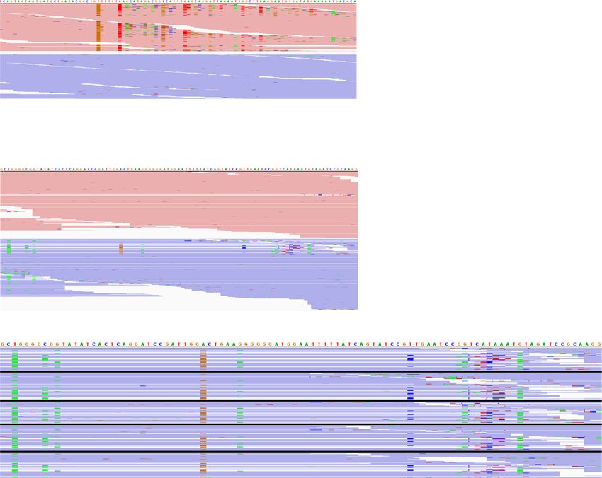
Fig. 2 Systematic errors in Illumina data. a, c Screenshots from the Integrative Genomics Viewer [37, 38] for
Ec-Hi2000-TruSeq (a) and Ec-Hi4000-Nextera (c). The forward strand is colored red and the reverse strand
blue. The bright colors mark substitution errors. b, d Amount of errors for all positions in the reference. e
Section from c with the same section from four technical replicates of Ec-Hi4000-Nextera (Ecoli1_L001):
Ecoli1_L002, Ecoli1_L003, Ecoli2_L001, Ecoli3_L001. The datasets are separated by thick black linesSchmeing and Robinson Genome Biology (2021) 22:67 Page 9 of 37
Heterozygous variants in diploid samples (Additional file 1: Figure S8h–j) and fragmented
references (Additional file 1: Figure S8c) also lead to reduced similarity to real data.
Coverage model
The coverage model defines the probabilities of where simulated reads start and end in
the simulated genome (template). It works on fragment sites, which are defined by their
reference sequence, start position, fragment length, and strand. Sites have been shown to
be a good choice to estimate GC bias [24]. Since in our model duplications are fragments
falling on the same site, the strand was added to make duplications strand-specific. Dur-
ing the statistics calculation, ReSeq determines all possible sites in a genome and counts
the read pairs mapping to them. Sites, where the true counts are likely to deviate from the
observed counts, e.g., repeat regions, are removed by looking at clusters of low mapping
quality (see the “Methods” section). During the simulation, repeats do not require special
consideration as long as they are part of the simulation template.
The model takes four different sources of bias into account: GC and flanking sequence
in a first step and fragment length and reference sequence in a second step. The flanking
bias arises from the nucleotides flanking the start and end of the fragment as a result
of the fragmentation process. We observed that their effect on the coverage is especially
pronounced if enzyme digestion is used (Additional file 1: Figure S9). The GC bias is
due to PCR [23], while the fragment-length bias results from the fragmentation and size
selection. Lastly, the reference-sequence bias represents the original abundance of the
sequence in the sample.
In the first step of the coverage estimation, the GC and flanking bias are fit to the sites
and their counts. Modeling the counts at each site with a Poisson would only account for
statistical duplications. Therefore, we use a negative binomial to additionally account for
PCR and optical duplications. Since coverage biases arise from different processes, we
assume independence and write the mean μn of the negative binomial as a product:
μn = Ñbseq (seqn )blen (lenn )bGC (GCn )bstart,n bend,n
with Ñ as the genome-wide normalization and the different b as the biases for this site.
The normalization parameter is of no further interest after the fit, leaving 128 rele-
vant parameters. The GC bias bGC (Fig. 3a) is binned by percent into 101 bins that are
described by a natural cubic spline with six knots, i.e. six degrees of freedom.
The flanking bias (Fig. 3b) has 120 parameters: one for each nucleotide across each of
thirty positions (10 bases before the fragment to 20 bases within). The flanking bias at the
start and end of the fragment use the same parameters due to their similarity (Additional
file 1: Figure S9), with the end reverse complemented to keep the meaning of positions
relative to the fragment. Since the best way of combining biases from individual positions
in the flank is a priori unknown, we tested the two simple options of a product and a sum
on datasets fragmented using mechanical forces (Ec-Hi2000-TruSeq) and enzymes (Ec-
Hi4000-Nextera). As seen in Fig. 3c, the predictions from the summation model nicely fit
to the observed count means, using 2 · 105 sites per bin.
To properly account for duplications, the dispersion has two parameters, α and β,
leading to the following mean-variance relationship:
σn2 = μn + αμn + βμ2n .Schmeing and Robinson Genome Biology (2021) 22:67 Page 10 of 37
Fig. 3 Coverage model. a GC bias for Ec-Hi2000-TruSeq at the four steps of the bias fit for 30 fits with
different fragment lengths. The red dots in the normalized panel are the median value and represent the final
result. The horizontal lines in the GC spline panel are the chosen knots for one example fragment length. b
Flanking bias. The effect of nucleotides in the genome relative to the fragment start or end with position 0
being the start/end. Negative positions are outside of the fragment. Only position − 3 to 11 are shown from
the total model that includes position − 10 to 19. Each box summarizes 30 to 40 fits with different fragment
lengths. The boxes are arranged around their true position for improved readability. The three datasets are all
created with Nextera adapters. c Comparison of combining the different positions in the flanking bias by a
product or a sum. Each dot is one bin of 2 · 105 fragment sites for one of 30 fits with different fragment
length. The fragment sites are ordered by their predicted mean counts μn before binning. The x-axis is the
mean of observed counts in the bin. The y-axis is the mean of predicted mean counts. For the sum the dots
scatter around the identity, while for the product a curve is visible. d, e The observed counts kn for the bins
defined in c are fitted with a negative binomial with constant dispersion r for Ec-Hi2000-TruSeq (d) and
Ec-Hi4000-Nextera (e). While Ec-Hi2000-TruSeq shows a significant slope and nearly no y-intercept,
Ec-Hi4000-Nextera shows the exact opposite
Figure 3d, e, where α is the y-intercept and β is the slope, demonstrates that both param-
eters are needed to properly simulate all datasets and duplication types, even if single
datasets need only one of the parameters (Additional file 1: Figure S10a) [39].
After the other biases have been fitted, ReSeq estimates the reference-sequence and
fragment-length biases by iteratively adjusting them to match the observed coverage.
To test the biases obtained by ReSeq, we use Bc-Hi4000-Nextera, Ec-Hi4000-Nextera,
and Rs-Hi4000-Nextera, which should have similar biases; and indeed, the flanking biases
do not vary much in those three datasets (Fig. 3b), despite the different median GC con-
tent of the underlying genomes (35%, 51%, and 69%). Furthermore, we clearly reproduce
previous findings for Nextera adapters [25], where the biases between a nucleotide and
its complement are very similar if mirrored around position 4 (e.g., A at 5 and T at 3).
The GC biases for the three datasets are compared in Figure S11 (Additional file 1),
where the spread between different fragment lengths highlights the lower confidence in
biases based on fewer sites. Bc-Hi4000-Nextera and Ec-Hi4000-Nextera look very similar,
except for low-confidence, GC-rich fragments. Rs-Hi4000-Nextera looks somewhat dif-
ferent, but its high-confidence region is poorly accessible by the other two datasets. The
reduced occurrence of AT-rich fragments (AT dropout) described in the literature [25] isSchmeing and Robinson Genome Biology (2021) 22:67 Page 11 of 37
also observed with the exception of Rs-Hi4000-Nextera, which has little power to detect
AT dropout due to its high median GC content. As another test, the biases were esti-
mated on simulated, uniformly distributed data, which results in the expected flat profile
(Additional file 1: Figure S12). The minor deviations for GC biases at the edges are due to
low amounts of available sites. Overall, the above tests show that this part of the coverage
model delivers accurate and consistent results.
Comparison of coverage distributions
Figure 4 shows ReSeq’s improvements over the uniform distribution (ART and BEAR) or
the sliding window approach (pIRS and NEAT), in terms of base-coverage distributions.
No other simulator shows consistently a good accordance with real data. In Ec-Hi2500-
TruSeq-asm (Fig. 4c), the median coverage provided as coverage parameter to ART, pIRS,
and NEAT is not a good estimator for the real coverage, because the duplicated regions
and the many very short hard-to-map contigs in the assembly reduce the median coverage
from 1011 to 13. Therefore, ART and pIRS do not have an expected peak, whereas NEAT’s
Fig. 4 Base-coverage distribution. Note that j BEAR was omitted due to excessive runtimes. k BEAR was
omitted, because it did not have a single proper pair mappedSchmeing and Robinson Genome Biology (2021) 22:67 Page 12 of 37
peak is at a very low coverage. ReSeq extracts the coverage itself and is therefore not
directly affected. BEAR requires the number of reads and is therefore also not affected,
but still does not show a peak at the correct coverage. In Figure S13 (Additional file 1),
the median coverage estimated from the mapping to the reference (Ec-Hi2500-TruSeq)
is provided to all simulators except BEAR. Since this is the only coverage parameter for
ART, it performs the same as in Ec-Hi2500-TruSeq. In contrast, pIRS and NEAT do not
manage to simulate a coverage that remotely resembles real data, because their GC-bias
estimation is not robust to fragmented references.
ReSeq’s negative binomial also captures the number of duplicated read pairs well
for most datasets (Fig. 5), despite a decrease in performance with increasing size and
complexity of the genome. A particular case are human samples, where the simulated
duplication numbers exceed the highest real ones, but only around 0.1% of the fragments
are affected for the most severe case in Hs-HiX-TruSeq (Fig. 5i). Other simulators do not
handle duplications and thus do not resemble real data (Fig. 5d–j, l), except for datasets
with low levels of duplication.
Fig. 5 Fragment duplication. The spike at 51 is an artifact of the counting that treats everything above 50 as
51. Note that c ART, pIRS, NEAT, and BEAR are omitted due to low coverage. j BEAR was omitted due to
excessive runtimes. k BEAR was omitted, because it did not have a single proper pair mappedSchmeing and Robinson Genome Biology (2021) 22:67 Page 13 of 37
Furthermore, ReSeq replicates the fragment-length distribution accurately (Additional
file 1: Figure S14) for two reasons: (i) it does not parameterize the distribution with a
Gaussian, which prevents ART, pIRS, and BEAR from capturing the long tail (Additional
file 1: Figure S14a–c, h–j, l); (ii) it is the only simulator that implements adapters, which
allows for fragment lengths below the read length (Additional file 1: Figure S14d–f, k).
BEAR also allows for shorter fragment lengths, but does so by trimming the read length
and thereby prevents benchmarks that require adapters to be present.
As a further test, we can again use the technical replicates of Ec-Hi4000-Nextera
(Ecoli1_L001). The correlation of the base coverage between Ecoli1_L001, Ecoli1_L002,
Ecoli1_L003, Ecoli2_L001, and Ecoli3_L001 can be seen as a gold standard of how
much the base coverage of simulations should be correlated to real data. We calcu-
lated the three pairwise Spearman correlations of replicates from the same lane and
from the same library, respectively, and compared them to the correlations of three
independent simulations based on Ec-Hi4000-Nextera. For the simulations, we calcu-
lated the pairwise Spearman correlations with themselves and the three correlations
with Ec-Hi4000-Nextera. Table 3 lists the averages of the calculated coverage correla-
tions. For each entry, one of the three corresponding correlations is plotted in Figure S15
(Additional file 1). The correlations highlight three major points. First, ReSeq strongly
increases the correlation between simulation and real data because, despite its high vari-
ance, the whole coverage distribution follows the real trend, which is not visible for other
simulators. Second, independent simulations from ReSeq approach the correlatedness of
real data, but do not populate the low- and high-coverage regions present in real data.
Only pIRS performs similarly, but with a correlation of 1, nearly all randomness seems to
be removed. Third, despite the major improvements, the correlation between ReSeq and
real data is still low and further improvements are possible.
Comparison of k-mer spectra
A good high-level summary statistic to represent a dataset of genomic reads is the k-mer
spectrum, which shows the systematic properties of errors (exponential decrease at low
frequencies) and the coverage distribution (shape and position of peaks) (see Sohn and
Nam Figure 4 [40]). Figure 6 (linear scale) and Figure S16 (log scale, Additional file 1) dis-
play the 51-mer spectra of the datasets and their simulations. The 31-mer and 71-mer
spectra (Additional file 1: Figure S17, S18) are qualitatively the same and the conclusions
drawn in this section are not specific for k = 51. The first row (Fig. 6a–c) is based on
high-coverage E. coli datasets sequenced on the older HiSeq 2000 and 2500 with TruSeq
Table 3 Average (pairwise) Spearman correlations of base coverage
Lane Library Real Simulation
Real 0.91 0.92 - -
ReSeq - - 0.23 0.81
ART - - 0.01 0.00
pIRS - - 0.12 1.00
NEAT - - 0.10 0.26
BEAR - - − 0.00 0.05
The bold numbers highlight the simulators, which are the closest to the correlatedness of real data in the given category. Lane: Ec-
Hi4000-Nextera (Ecoli1_L001) and replicates Ecoli1_L002 and Ecoli1_L003. Library: Ec-Hi4000-Nextera (Ecoli1_L001) and replicates
Ecoli2_L001 and Ecoli3_L001. Real: Ec-Hi4000-Nextera and three simulations. Simulation: Three simulations of Ec-Hi4000-NexteraSchmeing and Robinson Genome Biology (2021) 22:67 Page 14 of 37
Fig. 6 51-mer spectra of real and simulated data. The shape and position of peaks reflects the coverage
distribution, while the exponential decrease at low frequencies is defined by systematic errors. The black lines
show the minimum between the exponential decrease and signal peak for real data. The first value of R gives
the sum of relative deviations for frequencies (x) up to the minimum. The second value of R gives the sum of
absolute deviations for frequencies larger than the minimum. Both values are stated relative to ReSeq. When
the signal peak of the simulation does not exist or starts before the minimum in real data the values lose their
interpretability. This happens for ART (a, c), pIRS (c, d, l), NEAT (a, c-e, l), and BEAR (b, c, f–g, i, k–l)
adapters and includes the simulations trained on the fragmented assembly instead of the
reference (Fig. 6c). The second row’s bacteria datasets (Fig. 6d-f ) are all produced in a
single HiSeq 4000 run using Nextera adapters (enzyme fragmentation). They are ordered
from left to right by coverage ranging from high (508x) to very high (2901x) and by
genome complexity: single sequence (E. coli), two sequences where one is not present in
the data (B. cereus) and multiple sequences including plasmids of varying abundance (R.
sphaeroides). The plasmids cause multiple smaller peaks in the 51-mer spectrum with
lower frequencies than the main peak (Additional file 1: Figure S16f ). Additionally, espe-
cially in Bc-Hi4000-Nextera (Additional file 1: Figure S16e), we observe variants in the
bacteria populations that increase the 51-mer counts between the systematic errors and
the signal peak. Although NEAT and ReSeq accept Vcf files, which allows non-diploid
variants to be specified, we do not include them in the simulation. In the third row,Schmeing and Robinson Genome Biology (2021) 22:67 Page 15 of 37
we have low-coverage (31x-43x), diploid datasets sequenced on HiSeq X Ten machines
with TruSeq or related adapters. Here, we do include the variants in the simulations,
which results in a second peak in the 51-mer spectrum at half the frequency of the main
peak (Fig. 6h,i). Furthermore, the three genomes contain sequences with differences in
abundance: in At-HiX-TruSeq (Additional file 1: Figure S16g), we observe a second peak
at higher frequencies stemming from the mitochondria; in Mm-HiX-Unknown (Fig. 6h),
complex changes in the NIH3T3 cell line [41], including copy-number variations, broaden
the signal peak; and, in Hs-HiX-TruSeq (Fig. 6i), the X and Y chromosomes strengthen
the heterozygous peak at half the coverage of the main peak. The fourth row is a mix
of sequencers (NovaSeq, MiSeq, BGISEQ) run on different species (H. sapiens, E. coli,
A. thalina) with medium coverage(131x-194x). The diploid species were simulated with
variants.
BEAR does not produce a signal peak that matches the real signal’s shape or position in
any of the tested datasets. ART is consistently underperforming, for the coverage distri-
bution as well as for the systematic errors. Its error rate inflation for Ec-Hi2000-TruSeq
is causing the strong peak shift in the 51-mer spectrum (Fig. 6a). Notably, pIRS struggles
with datasets with Nextera adapters: for Ec-Hi4000-Nextera, it results in a rather flat peak
and an overabundance of high-frequency 51-mers (Fig. 6d), while it maintains a uniform
coverage distribution for the other Nextera datasets (Fig. 6e-f ).
ReSeq compares favorably for the coverage distributions of all datasets, except Ec-Mi-
TruSeq (Fig. 6a–j, l), and for the systematic errors of all datasets, except At-HiX-TruSeq
and At-BGI (Fig. 6a–f, h–k, Additional file 1: Figure S16a–f, h–k). Notably, ReSeq repro-
duces the coverage peak better on data with TruSeq adapters (Fig. 6a, b, g–j), compared
to Nextera adapters (Fig. 6d–f ). Furthermore, for all three HiSeq X Ten samples and the
BGISEQ sample (Fig. 6g–i, l), ReSeq slightly underestimates the coverage. This could be
manually corrected by specifying a parameter. For Ex-Mi-TruSeq, it is more complicated,
because the coverage distribution fits (Fig. 4k), but the k-mer peak does not (Fig. 6k).
A likely reason are large differences between the reference and the genome underlying
the data (for instance, a low mapping rate of 65%). Using the higher medium coverage
instead of ReSeq’s own estimation improves the 51-mer spectrum, but reduces the simi-
larity to real data for the base-coverage distribution (Additional file 1: Figure S19). Finally,
the exponential decrease is poorly reproduced in the low and medium coverage datasets
(Additional file 1: Figure S16g–l). We already saw that the systematic errors are harder to
replicate for diploid samples (Additional file 1: Figure S8g–j, l); additionally, the extremes
of the coverage peak, which are missing in simulations (Additional file 1: Figure S15c),
overlap more with the exponential decrease than in high coverage datasets.
Since for Ec-Hi2500-TruSeq-asm (Fig. 6c), the median coverage provided (as coverage
parameter to ART, pIRS, and NEAT) is a poor estimator, the median coverage esti-
mated from the mapping to the reference is provided to all simulators except BEAR for
Figure S20 (Additional file 1). For ART, the improved coverage removes nearly all perfor-
mance losses compared to Ec-Hi2500-TruSeq, which is not surprising, since only InDel
rates and the fragment-length parameters are taken from the assembly. Even though its
performance is still low, ART improves relative to pIRS and NEAT, because these two
do not cope well with the fragmented assembly and produce rather flat and broad peaks.
ReSeq’s coverage model also suffers from using the assembly instead of the reference, but
can still maintain a general resemblance to the real data.Schmeing and Robinson Genome Biology (2021) 22:67 Page 16 of 37
Fig. 7 Simulated contig N50 for real and simulated data. c preqc crashes for pIRS. f preqc crashes for pIRS
and ART
Comparison of assembly continuity
To check whether the improved representation in the k-mer spectrum has consequences
for applications, we ran the sga preqc module on all datasets and their simulations (Fig. 7).
The preqc module estimates the N50 (length of the shortest contig still necessary to cover
50% of the genome) of short-read assemblies for different k-mer lengths. Due to crashes,
Ec-Hi2500-TruSeq-asm is missing pIRS and Rs-Hi4000-Nextera is missing pIRS and ART.
For many datasets, ReSeq follows real data better than the other simulators (Fig. 7a–e).
In the others, namely the low- and medium-coverage HiSeq X Ten and NovaSeq datasets
(Fig. 7g–j), all simulators except BEAR perform equally, because the missed systematic
nature of errors and undetected diploid variants prevent ReSeq from delivering the same
performance. Only in Ec-Mi-TruSeq does ReSeq perform worse than NEAT and ART,
due to the discrepancy between mapped coverage and k-mer coverage. Setting the cov-
erage parameter to the median coverage as for the other simulators mitigates this effect
(Additional file 1: Figure S21). For Rs-Hi4000-Nextera, BEAR deviates drastically from
real data and other simulators (Fig. 7f ). Figure S22 (Additional file 1) shows the same plotSchmeing and Robinson Genome Biology (2021) 22:67 Page 17 of 37
without BEAR, but due to fluctuations in the real N50 values, no strong conclusions can
be drawn.
In Ec-Hi2500-TruSeq-asm (Fig. 7c), the coverage-parameter estimate from the assembly
strongly affects the N50 values of ART, pIRS, and NEAT. Providing the coverage estimate
from the reference to all simulators except BEAR (Additional file 1: Figure S23), mostly
reverts the drastic changes in N50. pIRS’s difference to real data only slightly increases,
compared to using the reference for the complete training (Ec-Hi2500-TruSeq: Fig. 7b),
while NEAT does not show the unexpected peak of N50 around k = 50 anymore, but
does not restore the slight resemblance to the real data it had in Ec-Hi2500-TruSeq, and
ART fully recovers the increase in N50 toward high k that has at least the same tendency
as real data. Noticeably, ReSeq’s N50 values stay close to the real ones no matter how it
was trained.
Comparison of cross-species simulations
An important property of trained profiles is that not only can they be used to simu-
late the original dataset, but also datasets with alternative templates. To test training
and simulation across species, we split six of the datasets into two groups with identi-
cal sequencer and fragmentation combinations. The datasets were simulated using the
median coverage, template, and variants from the simulated datasets; all other param-
eters and profiles were provided from another dataset within the group. The resulting
51-mer spectra are compared to those of the simulated datasets in Figure S24 (linear scale,
Additional file 1) and Figure S25 (log scale, Additional file 1). In the HiSeq 4000 group
with enzyme fragmentation, we used the profiles from Ec-Hi4000-Nextera to simulate
Bc-Hi4000-Nextera and Rs-Hi4000-Nextera and the profiles from Rs-Hi4000-Nextera
to simulate Ec-Hi4000-Nextera. The results highlight the difficulty of applying profiles
across genomes with very different GC content (Additional file 1: Figure S24a-c). In the
HiSeq X Ten group with mechanical fragmentation and genomes with similar GC con-
tent (Additional file 1: Figure S24d-f ), we used the profiles from Mm-HiX-Unknown to
simulate At-HiX-TruSeq and Hs-HiX-TruSeq and the profiles from Hs-HiX-TruSeq to
simulate Mm-HiX-Unknown.
Similar to the case of simulating the original datasets (Fig. 6), BEAR does not create a
signal peak that matches the real signal’s shape or position in any of the datasets, except
At-HiX-TruSeq (Additional file 1: Figure S24). ART is unaffected by the profile change,
but still shows low performance due to the uniformly distributed coverage. pIRS’s per-
formance on cross-species simulations is hard to judge on the Nextera datasets, because
pIRS already underperforms when reproducing the original Nextera datasets. For exam-
ple, pIRS on Ec-Hi4000-Nextera results in a rather flat peak (Fig. 6d) and simulating other
datasets from its profile results in no visible peak (Additional file 1: Figure S24b,c). How-
ever, for TruSeq adapters and genomes with similar median GC content, pIRS seems
to be unaffected by using profiles trained on a different species (Fig. 6g–i, Additional
file 1: Figure S24d-f )). This is not the case for NEAT, where in the HiSeq 4000 group,
minor peaks appear on the low-frequency side of the main peak (Additional file 1:
Figure S24c, S25a,c), and in the HiSeq X Ten group, an asymmetric signal peak with
a pronounced tail is visible in the simulations based on the Mm-HiX-Unknown profiles
(Additional file 1: Figure S24d,f ). This is likely caused by other sources of bias being
incorporated into the GC bias. ReSeq is missing the abundance information for theSchmeing and Robinson Genome Biology (2021) 22:67 Page 18 of 37
reference sequences and therefore does not correctly simulate the plasmids in Rs-Hi4000-
Nextera (Additional file 1: Figure S24c), the mitochondrial genome in At-HiX-TruSeq
(Additional file 1: Figure S25d), the copy-number variations in Mm-HiX-Unknown
(Additional file 1: Figure S24e), and the X and Y chromosome in Hs-HiX-TruSeq
(Additional file 1: Figure S24f ). This demonstrates how ReSeq nicely separates the
individual biases and produces results (Additional file 1: Figure S24) resembling the
original datasets (Fig. 6). On Mm-HiX-Unknown, we demonstrate that given the abun-
dance information, ReSeq again produces a coverage peak as good as the one from the
simulation trained on the original dataset (Additional file 1: Figure S26, Fig. 6h).
The assembly continuity seems to be unaffected by not incorporating abundance infor-
mation and most simulations perform as well or even slightly better (Additional file 1:
Figure S27b, d–f ) than with the profile from the original datasets (Fig. 7e, g–i). The
exception are simulating Ec-Hi4000-Nextera with the profile from Rs-Hi4000-Nextera
and vice versa. For Ec-Hi4000-Nextera, ReSeq, ART, and NEAT show a decrease in sim-
ilarity to the real data and only pIRS and BEAR improved, but they did not have any
resemblance to real data for the original profile (Additional file 1: Figure S27a, Fig. 7d).
For Rs-Hi4000-Nextera, the general trend is unclear, because only ReSeq and BEAR man-
age to create artificial datasets that can be evaluated with the preqc module in both cases
(Additional file 1: Figure S27c, S22, Fig. 7f ). ReSeq’s performance drops strongly in rel-
ative terms, but the absolute difference in N50 remains low. On the other hand, BEAR
changes from extremely high N50 values for the original profile to a flat N50 distribution
for the Ec-Hi4000-Nextera profile.
Looking at more detailed statistics, the quality values and error rates remain mostly
accurate (except for BEAR), but reflect the differences between datasets (Additional
file 1: Figure S28, S29, S30, S31). The systematic errors are reproduced by ReSeq
also for cross-species simulations, but the performance for the HiSeq 4000 datasets
with strongly varying median GC content (Additional file 1: Figure S32a-c) is reduced
compared to the simulation of the original datasets (Additional file 1: Figure S8d–f ). How-
ever, for the HiSeq X Ten datasets with similar median GC content, the performance
does not change (Additional file 1: Figure S32d–f, S8g–i). Finally, the base-coverage
distribution (Additional file 1: Figure S33) highlights again the effect of the miss-
ing abundance information for ReSeq and NEAT’s issue applying the GC bias across
species.
Comparison of computation requirements
Besides better representation of real data, computational requirements are also impor-
tant. Figure S34 (Additional file 1) shows the total CPU time, the elapsed time and the
maximum amount of memory used for the training and simulation steps of each simula-
tor for the eleven datasets. ReSeq lies on the high side of CPU time for training and in the
intermediate region for simulation (Additional file 1: Figure S34a, d). Noticeably, parts
of ReSeq’s CPU requirements scale with genome size instead of number of reads, which
leads to worse performance in lowly-covered genomes.
Due to ReSeq’s effective parallelization, its elapsed times are low for this benchmark
with 48 virtual CPUs (Additional file 1: Figure S34b,e). In contrast, the single-threaded
processes implemented in perl or python have strikingly high elapsed times. This is well
visible in Hs-HiX-TruSeq and applies to the training of pIRS (over a week), NEAT (severalSchmeing and Robinson Genome Biology (2021) 22:67 Page 19 of 37
days), and BEAR (half a week) as well as the simulation of NEAT (close to 2 weeks) and
BEAR (several weeks). For the simulation, NEAT provides a tool to split the template
and later merge the reads, which can be used for manual parallelization with multiple
instances to reduce the elapsed time to 10 h in this case.
Memory requirements remain mostly below 10GB for training (Additional file 1:
Figure S34c). The exceptions are pIRS needing around 20GB to train on human-sized
genomes and ReSeq requiring around 150GB for training on these datasets. However,
ReSeq’s memory consumption during training strongly depends on the amount of CPUs
used (Additional file 1: Figure S35). Therefore, the memory requirements can be reduced
substantially by a mixed setup, where only a single thread is used for the statistics cal-
culation and multiple threads are used for the probability estimation. Thus, if needed,
ReSeq can still fallback to time and memory requirements that are in the same range as
the simulators using single-threaded training scripts. For simulations (Additional file 1:
Figure S34f ), the memory requirements stay also below 10 GB, except for the multiple
instances approaches that require on human-sized genomes 35–90 Gb (ART) or 120Gb
(NEAT). Another exception is BEAR that needs close to 14 GB for Rs-Hi4000-Nextera
and around 100 GB for Mm-HiX-Unknown and Hs-HiX-TruSeq. In typical systems with
2–8 GB per core, BEAR’s high-memory requirements may block many CPUs additional
to the 2 used ones, which could lead to effective CPU times much higher than the values
in Figure S34d (Additional file 1).
Example: genuine comparison of short-read mappers
After comparing ReSeq to other simulators, we demonstrate its use in an example of
a simulation study, where the performance of two popular mapping algorithms, bwa
and bowtie2, is compared. For the simulation, we trained ReSeq either on bowtie2
or bwa mappings to verify that performance is not biased by the mapper used for
training.
As a first quality check, we compare mapping statistics between simulated and real data
for three datasets (Fig. 8a–c). In real data, the number of unmapped pairs and single reads
is higher compared to the simulation, which is most pronounced in Ec-Hi2500-TruSeq
(Fig. 8b), where the mapping of some reads is prevented by deviations between the ref-
erence genome and the true genome underlying the data. In contrast, simulated reads
are drawn directly from the reference template and thus do not exhibit mapping issues
caused by genome deviations. Furthermore, the bowtie2-based Ec-Hi2000-TruSeq simu-
lation (Fig. 8a) compared to the bwa-based simulation and real data has less unmapped
reads for bowtie2 and less soft-clipping, which could be a sign of underestimated adapter
content, but the truth data from the simulations show that the difference in adapter con-
tent can only account for less than 1/6 of the difference in unmapped reads. Finally, the
number of insertions and deletions varies in several cases (Fig. 8a–c), but for the general
comparison of mappers here, the differences are too low to influence the result.
As a next step, we compare the mapping-quality distributions between simulated and
real data (Fig. 8d–f ) and observe that the mapping rates increase in mostly identical steps,
when mapping quality requirements are lowered. The overall shifts in mapping rates are
an alternative representation of the different percentages of unmapped reads discussed
in the previous paragraph. A prominent feature not explained by the general shifts can
be seen in Ec-Hi2000-TruSeq (Fig. 8d), where the difference in mapping rate betweenSchmeing and Robinson Genome Biology (2021) 22:67 Page 20 of 37
Fig. 8 Comparison between bwa and bowtie2 on E. coli. Each dataset has simulations trained on mappings
from bwa and bowtie2. a–c Statistics of mapping outcomes. Bowtie2 does not clip and therefore has no
soft-clipped bases. d–f Mapping quality distribution. Mapping qualities are cumulative, i.e., all mapping
qualities at the given score or higher. Markers are only shown for mapping qualities 0,2,30,42 for bowtie and
0,1,30,60 for bwa. g–i Mapping accuracy for all mapping quality thresholds. Markers are only shown for
mapping qualities 0,2,30,42 for bowtie and 0,1,30,60 for bwa. Positives are mapped reads, which fulfill the
correctness criteria (TP) or do not (FP). Overlapping: True and mapped positions overlap independent of
strand. Correct_start: Perfect match of start position and strand. Correct: Perfect match of start and end
positions and strand. a, d, g Ec-Hi2000-TruSeq. b, e, h Ec-Hi2500-TruSeq. c, f, i Ec-Hi4000-Nextera
the two simulations is much more pronounced for high-quality mappings compared to
low-quality mappings. In light of the observed decrease in soft-clipped bases (Fig. 8a),
the mapping rate differences can be explained by a lower number of simulated reads
with many errors (> 10) for the bowtie2-based simulation compared to the bwa-based
(Additional file 1: Figure S36). We observe that bwa handles dense errors by clipping the
reads, while bowtie2 reduces the mapping quality.
Finally, we can use the truth from the simulations to calculate true positives (TP) and
false positives (FP) of read mapping (Fig. 8g-i). In Ec-Hi2000-TruSeq (Fig. 8g), we observe
strong differences in TPs between simulations, which are due to the different amount
of reads with many errors (Additional file 1: Figure S36) and we use the bwa-based
simulation.
Overall, we observe that in the case of strong adapter presence, bwa is the better choice
due to its soft-clipping capability (Fig. 8i), although bowtie2 allows better control over
FPs with adequate mapping quality thresholds in case both read ends are required to
map perfectly. Ec-Hi4000-Nextera also highlights how important adapter simulation is
to get an adequate mapping comparison (Additional file 1: Figure S37). In the datasets
with lower adapter content (Fig. 8g, h), the recommended mapper depends on the down-
stream application. If perfect mapping is required, bowtie2 is the better choice, since bwaYou can also read