Cambridge, MA 02138 May 2020 We are deeply grateful to Editor and two anonymous referees for very helpful comments. We thank Philip Bond, Matthieu ...
←
→
Page content transcription
If your browser does not render page correctly, please read the page content below
NBER WORKING PAPER SERIES

               TOKENOMICS: DYNAMIC ADOPTION AND VALUATION

                                     Lin William Cong
                                          Ye Li
                                        Neng Wang

                                     Working Paper 27222
                             http://www.nber.org/papers/w27222

                    NATIONAL BUREAU OF ECONOMIC RESEARCH
                             1050 Massachusetts Avenue
                               Cambridge, MA 02138
                                    May 2020

We are deeply grateful to Editor and two anonymous referees for very helpful comments. We
thank Philip Bond, Matthieu Bouvard, Jaime Casassus, Tom Ding, Alex Frankel, Zhiguo He,
Dirk Jenter, Andrew Karolyi, Yongjin Kim, Michael Sockin, Aleh Tsyvinski, Pietro Veronesi,
Johan Walden, Larry Wall, Randall Wright, Yizhou Xiao, and seminar and conference
participants at AEA/AFE (Atlanta), Ansatz Capital, Ant Financial, Atlanta Fed & GSU CEAR
Conference on Financial Stability Implications of New Technology, Baidu Du Xiaoman
Financial, CEPR ESSFM Gerzensee, Chicago Booth, City University of Hong Kong
International Finance Conference, CKGSB, CMU Tepper (Business Technology/
Information Systems), Emerging Trends in Entrepreneurial Finance Conference, Finance
UC 14th International Conference, Georgetown, HKUST Finance Symposium, JOIM
Conference on FinTech, LeBow/GIC/FRB Conference on Cryptocurrencies in the Global
Economy, London Finance Theory Group Summer Conference, Luohan Academy First Digital
Economy Conference (joint with Alibaba Damo Academy), National University of Singapore,
NYU Stern FinTech Conferece, Norwegian School of Economics, PBC School of Finance,
the 3rd Pensions and ESG Forum, RCFS/RAPS Conference in Baha Mar, 3rd Rome Junior
Finance Conference, SEC DERA, Shanghai Forum, Stanford SITE, Tokenomics International
conference on Blockchain Economics, Security and Protocols, University of Cincinnati,
University of Washington Foster, University of Zurich/ETH, and UT Dallas Finance Conference
for helpful comments. Cong gratefully acknowledges Xiao Zhang for excellent research
assistance and the Center for Research in Security Prices for financial support. The views
expressed herein are those of the authors and do not necessarily reflect the views of the
National Bureau of Economic Research.

NBER working papers are circulated for discussion and comment purposes. They have not been
peer-reviewed or been subject to the review by the NBER Board of Directors that accompanies
official NBER publications.

© 2020 by Lin William Cong, Ye Li, and Neng Wang. All rights reserved. Short sections of text,
not to exceed two paragraphs, may be quoted without explicit permission provided that full
credit, including © notice, is given to the source.
Tokenomics: Dynamic Adoption and Valuation
Lin William Cong, Ye Li, and Neng Wang
NBER Working Paper No. 27222
May 2020
JEL No. E42,G12,L86

                                         ABSTRACT

We develop a dynamic asset-pricing model of cryptocurrencies/tokens that allow users to conduct
peer-to-peer transactions on digital platforms. The equilibrium value of tokens is determined by
aggregating heterogeneous users' transactional demand rather than discounting cashflows as in
standard valuation models. Endogenous platform adoption builds upon user network externality
and exhibits an S-curve—it starts slow, becomes volatile, and eventually tapers off. Introducing
tokens lowers users' transaction costs on the platform by allowing users to capitalize on platform
growth. The resulting intertemporal feedback between user adoption and token price accelerates
adoption and dampens user-base volatility.

Lin William Cong                                Neng Wang
Cornell University                              Columbia Business School
Ithaca, NY 14853                                3022 Broadway, Uris Hall 812
will.cong@cornell.edu                           New York, NY 10027
                                                and NBER
Ye Li                                           nw2128@columbia.edu
The Ohio State University
Fisher College of Business
2100 Neil Ave
Fisher Hall 836
Columbus, OH 43210
li.8935@osu.edu
1 Introduction
Blockchain-based applications and cryptocurrencies have recently taken a center stage
among technological breakthroughs in finance. The global market capitalization of cryp-
tocurrencies has grown to hundreds of billions of US dollars. Nevertheless, academics, prac-
titioners, and regulators have divergent views on how cryptocurrencies derive their value.
In this paper, we provide a fundamentals-based dynamic valuation model for cryptocur-
rencies. We focus on the endogenous formation of a digital marketplace or network (“the
platform”) where its native cryptocurrency settles transactions and derives its value from
underlying economic activities on the platform. To distinguish from cryptocurrencies as
general-purpose medium of exchange, we shall refer to platform-specific currencies as to-
kens. In contrast to financial assets whose values depend on cash flows, tokens derive value
by enabling users to conduct economic transactions on the digital platform.
Our model captures two key features shared by a majority of tokens. First, they are the
means of payment on platforms that support specific economic transactions. For example,
Filecoin is a digital marketplace that allows users to exchange data storage space for its
tokens (FIL). Another example is Basic Attention Token (BAT): advertisers use BATs to
pay for their ads, publishers receive BATs for hosting these ads, and web-browser users
are rewarded BATs for viewing these ads. Second, user adoption exhibits network effects.
In both examples, the more users the platform has, the easier it is for any user to find a
transaction counterparty, and the more useful the tokens are. Our model also applies to
tokens used on centralized platforms such as those being developed by platform businesses.1
Consequently, the market price of tokens and the platform user base (i.e., the total
number of platform users) naturally arise as two key endogenous variables in our model.
Our equilibrium token pricing formula exhibits three desirable features. First, token value
depends on the platform’s productivity, which captures the platform’s functionality and
other related factors (e.g., technological and regulatory changes). Second, the user base
enters positively into the pricing formula, capturing the positive network externality of user
1
Examples include online social networks (e.g., QQ coins on Tencent’s messaging platform) and online
games (e.g., Linden dollar for Second Life and WoW Gold for World of Warcraft).
1adoption. Third, user heterogeneity matters for both platform adoption and token pricing.
Moreover, we clarify the roles of tokens in platform adoption by comparing token-based
platforms and platforms that settle transactions with the numeraire consumption goods.
Using the numeraire goods as means of payment incurs a carry cost, the forgone return from
investing in financial assets. In contrast, introducing tokens encourages early adoption of
productive platforms, because agents expect token price appreciation, and thus, effectively
face a lower carry cost of using tokens for transactions. The expectation of future token
price change also stabilizes user adoption in the presence of platform productivity shocks.
Specifically, we consider a continuous-time economy with a continuum of agents who dif-
fer in their transaction needs (i.e., types) on the platform. We broadly interpret transactions
as including value transfers (e.g., Filecoin and BAT) and smart contracting (e.g., Ethereum).
Accordingly, we model an agent’s utility flow from platform transactions as a function of
platform productivity that evolves exogenously, her type, the user base, and the real (nu-
meraire good) value of the agent’s token holdings (“real token balance”). Importantly, this
flow utility increases with the user base, capturing the network effects. We characterize the
Markov equilibrium with platform productivity being the state variable. The model has two
key endogenous variables, the user base and token price.
In our model, agents make a two-step decision on (1) whether to adopt by paying a
participation cost to become a platform user, and if so, (2) the real token balance. The
token market clears by equating the agents’ demand and the fixed supply. A key insight of
our model is that users’ adoption decision exhibits not only static complementarity through
the flow utility of platform transactions but also an inter-temporal complementarity via the
carry cost of holding tokens that depends on the endogenous variation of token price.
Holding tokens as means of payment incurs a carry cost that is the forgone return from
investing in financial assets. However, on a promising platform with a positive productivity
drift, such cost is partly offset by the expected token price appreciation. Given a fixed supply
of tokens, the prospective growth of user base driven by productivity growth leads agents
to expect more users in the future and thus a stronger demand for tokens, which implies
an increase of token price. As such, even though users forgo the financial assets’ returns by
2holding tokens to transact, they are compensated by the expected appreciation of tokens.
Introducing tokens also stabilizes the user base, making it less sensitive to platform pro-
ductivity shocks. Consider a platform with growing yet stochastic productivity. A negative
productivity shock reduces users’ transactional utility and thus lowers the user base. This
negative effect is mitigated by an increase in the expected token price appreciation. A lower
current level of adoption implies a larger expected token price appreciation because more
users can be brought onto the platform in the future. Consequently, the effective token carry
cost declines, encouraging adoption. Similarly, a positive productivity shock directly in-
creases adoption, but its effect is dampened because the pool of potential newcomers shrinks
and the expected token price appreciation declines, resulting in a greater effective carry cost.
In the Markov equilibrium, our tokenized economy features an S-curve of user adoption
– as the platform productivity grows, the user base expands slowly, and then the expansion
speeds up before eventually tapering off near full adoption. We show that the user base
is larger and more stable than that of a tokenless platform that has the same productivity
process but uses the numeraire goods as means of payment.
We derive an equilibrium token pricing formula that incorporates endogenous network
effects in an otherwise canonical Gordon growth formula. Token valuation boils down to
solving an ordinary differential equation subject to intuitive boundary conditions. Just as
tokens affect the user-base dynamics, endogenous adoption is critical for understanding major
asset-pricing issues surrounding tokens.
First, the network effects imply a large cross-sectional variation in token price among
platforms in early stages of adoption. Second, adoption externality amplifies the impact
of productivity shocks on token price, creating “excess volatility”(e.g., Shiller, 1981). The
amplification is even stronger when we allow the productivity drift to increase with the
user base — a form of community bootstrapping that practitioners emphasize. Finally,
by allowing the productivity beta (systematic risk) to increase with adoption, our model
generates an initial rise of token price followed by a decline and eventual stabilization, broadly
consistent with the observed “bubbly” price dynamics. These results are in line with evidence
(e.g., Liu and Tsyvinski, 2018; Shams, 2019).
3In sum, our model features rich interactions between financial markets and the real
economy: the financial side operates through the endogenous determination of token prices,
whereas the real side manifests itself in the user adoption. By trading in the token market,
users profit from platform growth and effectively bear a reduced carry cost of conducting
transacting.2 For payment platforms, the prominent adoption problem in platform economics
(e.g., Rochet and Tirole, 2006) is naturally connected with the carry cost in the classic models
of money as transaction medium (e.g., Baumol, 1952; Tobin, 1956). Comparing with the
traditional user subsidies, we demonstrate tokens’ advantages in accelerating and smoothing
adoption. This new solution is often based on blockchains: decentralized consensus allows
the token supply to be credibly fixed, and thus, anchoring the token price to users’ demand.3
Related Literature. Among early economic studies on blockchain games and consensus
generation mechanisms, Biais, Bisiere, Bouvard, and Casamatta (2019) and Saleh (2017) an-
alyze mining/minting games in Proof-of-Work- and Proof-of-Stake-based public blockchains;
Easley, O’Hara, and Basu (2019), Huberman, Leshno, and Moallemi (2019), and Cong, He,
and Li (2018) study the market structure of miners; Cong and He (2018) examine the impact
of decentralized consensus on industrial organization. We differ by focusing on token users’
trade-off and the resulting dynamic interaction between platform adoption and token pricing
that apply to both centralized and decentralized platforms.
We connect platform economics and asset pricing by demonstrating that the token price is
anchored upon the platform-specific convenience yield (transactional value). Our treatment
of convenience yield is related to Krishnamurthy and Vissing-Jorgensen (2012) and earlier
studies. Our contribution is to incorporate user network effects in the convenience yield,
and study the implications on platform adoption and token pricing. We emphasize agent
heterogeneity and its asset-pricing implications. Instead of balance-sheet crises (e.g., He and
Krishnamurthy, 2011, 2013; Brunnermeier and Sannikov, 2014), we model the heterogeneity
2
Our model has complete information. Token capitalizes the otherwise non-tradable growth of platform
user base, and thereby, accelerates adoption under network effects. This is distinct from the informational
effects of financial markets that feeds back into the real activities (see Bond, Edmans, and Goldstein, 2012).
3
As pointed out by Hinzen, John, and Saleh (2019), the decentralized consensus often comes with a cost
of payment delays for proof-of-work blockchains. Computer scientists and economists are active in studing
alternative protocols (e.g., Saleh, 2017; Fanti, Kogan, and Viswanath, 2019).
4of platform users and the resulting endogenous growth of user base. In our model, platform
users expect profits from selling tokens to future users. This mechanism is related to but
different from Harrison and Kreps (1978) and Scheinkman and Xiong (2003) as the expected
capital gain in our model is due to the growth of user base rather than heterogeneous beliefs.
We do not analyze the implications of blockchain technology on general-purpose curren-
cies and monetary policies (e.g., Balvers and McDonald, 2017; Raskin and Yermack, 2016;
Garratt and Wallace, 2018; Schilling and Uhlig, 2018). Instead, we focus on the endogenous
interaction between token pricing and user adoption on platforms that serve niche markets
with time-varying productivity. Therefore token pricing is anchored upon the platform’s
productivity and the popularity of specific economic transactions it supports, such as adver-
tisement (BAT) and digital storage (Filecoin).
Among contemporary theories featuring token valuation in static settings, Sockin and
Xiong (2018) study tokens as indivisible membership certificates for agents to match and
trade with each other; Li and Mann (2018) argue that initial token offering allows agents to
coordinate by costly signaling through token acquisition; Pagnotta and Buraschi (2018) study
Bitcoin pricing on exogenous user networks; Catalini and Gans (2018) examine developers’
pricing of tokens to fund projects and aggregate information; Chod and Lyandres (2018)
contrast security token offerings with traditional financing.4 Our paper is the first to clarify
the role of tokens in capitalizing the endogenous platform growth, and thereby, reducing
agents’ effective carry cost of holding the transaction medium.5
In dynamic settings, Athey, Parashkevov, Sarukkai, and Xia (2016) emphasize the role of
learning in agents’ decisions to use Bitcoin absent stochastic platform productivity and user
network externality; Biais, Bisière, Bouvard, Casamatta, and Menkveld (2018) emphasize
the fundamental value of Bitcoin from transactional benefits; Fanti, Kogan, and Viswanath
(2019) provide a valuation framework for Proof-of-Stake (PoS) payment systems; Goldstein,
Gupta, and Sverchkov (2019) study initial token offerings that allow monopolistic platforms
4
Tokens in our model facilitate transactions. They should be distinguished from security tokens that
represent claims on issuers’ cashflows or rights to redeem products/services (e.g., Slice and Siafund tokens).
5
The carry cost features prominently in classic models of money demand (e.g., Baumol, 1952; Tobin,
1956) and recent literature of cash management (e.g., Alvarez and Lippi, 2013; Bolton, Chen, and Wang,
2011; Décamps, Mariotti, Rochet, and Villeneuve, 2011; Li, 2017; Lucas and Nicolini, 2015).
5to credibly commit to long-run competitive pricing of services. We differ by studying the
joint determination of user adoption and token valuation in a framework that highlights
user heterogeneity, network externalities, and most importantly, inter-temporal feedback
effects. Moreover, our model is applicable to platforms owned by trusted third parties and
permissioned blockchains as well as permissionless blockchains.
In the remainder of the article, Section 2 sets up the model, and 3, and 4 solve the
tokenless and tokenized economies, respectively. Section 5 discusses how tokens affect user
adoption and how endogenous adoption affects token price; Section 6 discusses alternative
solutions to platform adoption and trade-offs between scale and decentralization that can
potential limit the application of blockchain technologies in supporting tokenized platforms.
2 A Model of Platform Economy
Consider a continuous-time economy where a continuum of agents of unit measure con-
duct peer-to-peer transactions on a blockchain platform or a general digital marketplace.
2.1 Platform and Agents
The platform is characterized by At , the productivity that evolves according to a geo-
metric Brownian motion:
dAt
bA dt + σ A dZbtA ,
=µ (1)
At
where ZbtA is a standard Brownian motion under the physical measure and µ
bA and σ A are
constant parameters. We interpret At broadly. A positive shock to At can reflect technolog-
ical advances, favorable regulatory changes, growing users’ interests, and increasing variety
of activities feasible on the platform.
Preferences for platform transactions. The platform allows agents to conduct transac-
tions that are settled via a medium of exchange. We consider two cases for the medium: the
generic good, which is the numeraire, and the local platform currency (token).
We use xi,t to denote the value of agent i’s holdings of medium of exchange in units of the
numeraire good. Conditioning on participating on the platform, a platform user i derives a
6utility flow from her holdings of the medium of exchange, xi,t ,
dvi,t = (xi,t )1−α (Nt At eui )α dt − φdt − xi,t rdt . (2)
Next, we explain the three terms in (2) and later discuss agents’ participation decision.
The first term,
ui α
x1−α
i,t (Nt At e ) dt, (3)
is the transactional benefits of xi,t , where Nt is the platform user base, ui is the agent’s
type, At measures platform productivity, and α ∈ (0, 1) is a constant.6 Let Ut denote the
set of participating agents (with xi,t > 0), so formally, Nt ∈ [0, 1] is the measure of Ut . We
choose this specification of utility flow with the following considerations. First, the utility
flow increases in Nt . It captures the positive user network effect, as it is easier to find a
transaction counterparty in a larger community. Second, the marginal utility decreases with
xi,t , captured by α > 0. The exponents of xi,t and Nt At eui sum up to one for analytical
convenience. Third, agents’ transaction needs (or types), ui , are heterogeneous.7 Let G (u)
and g (u) denote the cross-sectional cumulative distribution function and density function of
ui , respectively. Both are continuously differentiable over the finite support [U , U ].
To realize the transaction benefits given in (3), the agent needs to incur a flow cost φ
per unit of time for platform participation corresponding to the second term in (2). For
example, transacting on the platform takes effort and attention. At any time t, agents may
choose not to participate and then collect no utility. Naturally, agents with sufficiently high
ui choose to join the platform, while agents with sufficiently low ui do not participate.
In addition to φ, the agent has to incur an opportunity cost of rxi,t per unit of time
to realize the transactional benefits in (3). This cost is similar to those induced by the
cash-in-advance constraints in monetary models where the opportunity costs of conducting
transactions is the forgone interest payments on the money balance (e.g., Galı́, 2015; Walsh,
6
Appendix A contains a theoretical foundation for this reduced-form flow utility.
7
For payment blockchains (e.g., Ripple), a high value of ui reflects agent i’s urge to conduct an in-
ternational remittance. For smart-contracting blockchains (e.g., Ethereum), ui captures agent i’s project
productivity. For decentralized computation (e.g., Dfinity) and data storage (e.g., Filecoin) applications, ui
corresponds to the need for secure and fast access to computing power and data.
72003). It also resembles the carry cost of cash holdings in corporate finance models that
emphasize external financing frictions (e.g., Bolton, Chen, and Wang, 2011; Li, 2017).
Valuing utilities from platform transactions. Because we consider a dynamic economy
of infinite horizon, the valuation of flow utilities from platform activities requires a stochastic
discount factor (SDF). For tractability, we consider the following widely-used specification
of SDF, which we denote by Λ:
dΛt
= −rdt − ηdZbtΛ , (4)
Λt
where r is the risk-free rate and η is the price of risk for systematic shock ZbtΛ under the
physical measure.8 The SDF is typically linked to agents’ consumption dynamics, so by
specifying an exogenous SDF, we assume that agents’ utility from platform activities consti-
tutes only a small part of their total utility. This echoes the models of an individual firm’s
valuation where an exogenous SDF is directly parameterized (Chapter 7, Campbell, 2017).
Let ρ denote the instantaneous correlation between the SDF shock and the platform
productivity shock At . A positive ρ implies a positive beta (Duffie, 2001). Indeed, the
usefulness and quality of a particular platform evolves with the economy, as agents discover
new ways to utilize the technology, which in turn depends on the progress of complementary
technologies. Macro and regulatory events may also affect the usage of a platform.
It is more convenient to solve our model via the change-of-measure technique widely used
in the derivatives pricing literature (Duffie, 2001). By Girsanov’s Theorem, we know that
under the risk-neutral measure, the Brownian motion driving the SDF is ZtΛ that satisfies
dZtΛ = dZbtΛ + ηdt. (5)
Therefore, under the risk-neutral measure, At follows
dAt
bA dt + σ A dZbtA = µ
=µ bA − ηρσ A dt + σ A dZtA ≡ µA dt + σ A dZtA . (6)
At
8
The standard no-arbitrage argument implies that the drift of the SDF has to equal to the negative
interest rate. See Duffie (2001) for a textbook treatment.
8Let yi,t denote agent i’s (undiscounted) cumulative payoff from platform activities, which
depends on dvi,t (the transactional benefits defined in (2)) and may differ on platforms with
b and E denote the
and without token as medium of exchange as will be specified shortly. Let E
expectation under the physical and risk-neutral measure, respectively. Agent i maximizes
her life-time payoff, Z Z ∞
∞
b Λt −rt
E dyi,t = E e dyi,t . (7)
0 Λ0 0
This equality follows from the change-of-measure technique. Throughout the remainder of
our paper, we conduct our analysis under the risk-neutral measure unless stated otherwise.
2.2 Tokenless and Tokenized Economies
Tokenless economy. On platforms with transactions settled by the numeraire good, agent
i’s utility flow only depends on whether she chooses to be a platform user, and if she does,
the transactional benefits of holding xi,t units of goods as means of payment:
dyi,t = max {0, max dvi,t } (8)
xi,t
1−α ui α
= max 0, max (xi,t ) (Nt At e ) − φ − rxi,t dt . (9)
xi,t
Here, the inner “max” operator gives the conditional demand xi,t if participating and the
outer “max” operator reflects agent i’s option to leave the platform and obtain zero profit.
This tokenless model is analogous to the standard models of money holdings (e.g., Ljungqvist
and Sargent, 2004), given that the real value of money balance, xi,t , generates a flow utility via
(xi,t )1−α (Nt At eui )α dt but induces a cost of forgone interests via xi,t rdt. Our novel modeling
ingredient is the user network effect—the positive externality of agents’ adoption decision—
which is a defining feature of digital platforms.
Tokenized economy. In what follows, we introduce a native (crypto)currency on the
platform, i.e., the token. To conduct transactions on the platform, users are required to use
9tokens.9 The value of agent i’s token holdings, xi,t , satisfies the following identity:
xi,t = Pt ki,t , (10)
where Pt is the token price in terms of the numeraire good and ki,t is the units of tokens.
The real (numeraire) value, xi,t = Pt ki,t , rather than the token units, ki,t , appears in the
transactional benefits because the transaction utility depends on the numeraire value of
goods and services that are transacted as in the standard monetary economic models.
Without loss of generality, we write the equilibrium token price process as follows under
the risk-neutral measure:
dPt = µ et dZtA
et dt + σ (11)
= Pt µPt dt + Pt σtP dZtA . (12)
Here, µ et can be any admissible stochastic processes. (12) is a re-writing of (11) where
et and σ
et = Pt µPt
µ and et = Pt σtP ,
σ (13)
and µPt and σtP can follow any admissible processes. We choose to work with µPt and σtP
rather than µ et , because the former set of notations is more convenient especially when
et and σ
we analyze our model’s asset-pricing predictions such as the expected token return and token
return volatility. But we could have used µ et to obtain the same solution.10
et and σ
Conditional on participating on the platform, agent i derives a total payoff that includes
the transactional benefits of token holdings, i.e., dvi,t , and also the investment payoff due to
endogenous token price change:
dvi,t + ki,t Et [dPt ] . (14)
9
In Appendix D, we generalize our model to incorporate agents’ endogenous decisions on whether to use
the numeraire good or token as medium of exchange, and show that our results are robust.
10
Proposition B1 in Appendix B shows that Pt > 0Pin equilibrium. Therefore, since Pt > 0, we can uniquely
infer µPt , σ P
t from (e
µ t , σ
e t ) or infer (e
µ t , σ
e t ) from µ t , σt
P
, so these two sets of notations are equivalent.
10By substituting ki,t = xi,t /Pt into (14), we rewrite the total payoff:
Et [dPt ]
dvi,t + xi,t . (15)
Pt
Using the definition µPt dt ≡ E [dPt ] /Pt , we can write the the total payoff as
P
dyi,t = max 0, max dvi,t + xi,t µt dt , (16)
xi,t
where the outer max accounts for agent i’ option to leave the platform and achieve zero
profit. In contrast to (8) of the tokenless economy that contains only dvi,t (the transactional
benefits), token introduces an additional term xi,t µPt dt due to the endogenous price variation.
By substituting (2) into (16), we express dyi,t explicitly as follows:
1−α ui α
dyi,t = max 0, max (xi,t ) (Nt At e ) − φ − r − µPt xi,t dt. (17)
xi,t
Introducing tokens changes the unit carry cost for holding transaction medium from rdt to
r − µPt dt. Agents must hold a medium of exchange ( the numeraire good in the tokenless
economy, or token in the tokenized economy) for dt to conduct transactions.11 During this
holding period, in addition to incurring the opportunity cost of forgone interests, agents in
the tokenized economy are exposed to the endogenous variation of token price. This feature
is absent in our tokenless economy.
Markov equilibrium. We study a Markov equilibrium with At , the platform productivity,
as the state variable whose dynamics generate the rational-expectation agents’ information
filtration. To focus on the dynamics of user adoption and demand, we fix the token supply
11
In blockchain-based systems, the holding period naturally arises because forging the ledger of transactions
takes time. For example, the Bitcoin blockchain requires 10-11 minutes to generate consensus on transactions.
This confirmation period is necessary for the finality of transactions as shown by Chiu and Koeppl (2017).
11to a constant M .12 The market clearing condition is
Z
M= ki,t di, (18)
i∈[0,1]
where for those who do not participate, ki,t = 0.
Definition 1. A Markov equilibrium with state variable At is described by agents’ decisions
and equilibrium token price such that the token market clearing condition given by (18) holds
and agents optimally decide to participate (or not) and choose token holdings.
3 Solution: Tokenless Economy
In our tokenless economy, the numeraire good is the medium of exchange. Conditional
on joining the platform (i.e., xi,t > 0), the agent chooses xi,t to maximize (2), which implies:
α
Nt At e u i
(1 − α) = r, (19)
xi,t
the marginal benefit from transaction is equal to the carry cost of forgone interests on xi,t .
Rearranging the optimality condition, we have:
1/α
ui,t 1−α
x∗i,t = Nt At e (20)
r
and the maximized profit from participating on platform is then:
" 1−α #
1−α α
dvi,t = Nt At eui α − φ dt. (21)
r
12
This captures the majority real-world applications. More generally, blockchain technology allows supply
to be based on explicit rules. This can be accommodated in the model by adding in an exogenous token
inflation or deflation rates that are orthogonal to the endogenous adoption and token demand dynamics.
12An agent participates only when dvi,t given in (21) is positive. That is, agent i participates
if and only if ui ≥ uN T NT
t , where ut is the endogenous threshold given by:
φ 1−α 1−α
uN
t
T
= − ln (Nt ) + ln − ln . (22)
At α α r
Here, the superscript “N T ” refers to the equilibrium value of the “no-token” (tokenless)
economy. Given the distribution of ui , G (ui ), the user base is thus given by:
φ 1−α 1−α
NtN T =1−G uN
t
T
= 1 − G − ln (Nt ) + ln − ln . (23)
At α α r
(22) and (23) jointly determine uN
t
T
and NtN T as functions of At .
Proposition 1 (Tokenless Equilibrium). In the Markov equilibrium with At being the
state variable, the user base NtN T and user type threshold uN
t
T
solve (22) and (23). Addi-
tionally, the user base, NtN T , increases in At if the cross-sectional distribution of agent type,
G (u), has an increasing hazard rate.
4 Solution: Tokenized Economy
Now consider a tokenized platform. As platform productivity At is the state variable,
all endogenous variables are functions of At in equilibrium. For example, Pt = P (At ). By
applying Itô’s lemma to Pt = P (At ), we obtain:
1 ′′ A
A 2
′
dPt = dP (At ) = P (At )At µ + P (At ) At σ dt + P ′ (At ) At σ A dZtA . (24)
2
By matching the coefficients of dt and dZtA to (12), we obtain µPt and σtP as functions of At :
P ′ (At ) 1 P ′′ (At ) 2
µPt = µP (At ) = At µ A + At σ A . (25)
P (At ) 2 P (At )
and
P ′ (At )
σtP = σ P (At ) = At σ A . (26)
P (At )
13With tokens, agent i’s decision on the real balance of medium of exchange, inside the
inner max operator in (17), is similar to (19) of the tokenless economy, but with tokens, the
effective carry cost is now r − µPt and the optimality condition agents’ token balance is:
α
N t At e u i
(1 − α) = r − µP (At ) , (27)
x∗i,t
where the marginal benefit of transaction is equal to the carry cost. Rearranging the equa-
tion, we have:
α1
ui 1−α
x∗i,t = Nt At e . (28)
r − µP (At )
the maximized profit from participating on platform is then
" 1−α #
[dPt ] 1−α α
max dvi,t + xi,t Et = Nt At e u i α − φ dt. (29)
xi,t Pt r − µP (At )
Substituting x∗i,t given in (28) into (17), we obtain the following user-type cutoff threshold
φ 1−α 1−α
ut = − ln (Nt ) + ln − ln , (30)
At α α r − µP (At )
and because only agents with ui ≥ ut will participate, the user base is then given by
Nt = 1 − G (ut ) . (31)
Equations (30) and (31) solve ut = u (At ) and Nt = N (At ) as functions of At .
Next, we derive an equilibrium token pricing formula. By using ki,t = xi,t /Pt and substi-
tuting (28) into the market clearing condition (18), we obtain:
α1
N (At ) S (At ) At 1−α
Pt = , (32)
M r − µP (At )
where Z U
St ≡ S (At ) = eu dG (u) (33)
u(At )
14is the sum of all participating agents’ eui , measuring the aggregate transaction needs. Indus-
try practices broadly corroborate the pricing formula (32). For example, as proxies for Nt
and St respectively, daily active addresses (DAA) and daily transaction volume (DTV) are
featured prominently in practitioners’ token valuation framework.13 But instead of heuristi-
cally aggregating such inputs into a pricing formula, we derive the token pricing formula as
equilibrium outcome together with endogenous user adoption.
By substituting (25) into the market clearing condition (32), we obtain:
α
1 2 N (At )S(At )At
rP (At ) = P (At ) At µ + P ′′ (At ) At σ A + (1 − α)
′ A
P (At ) . (34)
2 P (At )M
While our token pricing equation (34) may appear similar to the Black-Scholes-type
differential equation for derivatives pricing, the underlying economic force in our model is
α
N t St A t
different. The “flow” term, (1 − α) Pt M P (At ), in (34) comes from rearranging the
market clearing condition (32) and reflects the aggregation of agents’ transactional demand
for tokens. The Black-Scholes equation does not feature such a flow term. Moreover, the
Black-Scholes equation has a “theta” term – the variation of derivative value over time –
because of finite maturity, while (34) does not have such term because token does not have
maturity. Finally, platform productivity, At , the underlying fundamental that drives token
price, is not tradable, so the coefficient on P ′ (At ) is µA At , the drift of At under the risk-
neutral measure, instead of r in the case of derivatives on tradable underlying assets whose
risk-adjusted return must be r.14
We solve the preceding ODE for P (At ) with the following boundary conditions. The
lower boundary is given by:
lim P (At ) = 0 . (35)
At →0
As At = 0 is an absorbing state, the platform is not productive and no agent participates.
Therefore, the token price is zero. When At is sufficiently high, all agents participate. The
13
See, for example, the articile on token valuation, Today’s Crypto Asset Valuation Frameworks, by Ashley
Lannquist at World Economic Forum (Blockchain and Digital Currency).
14
Appendix F2 provides a more detailed comparison between our token pricing equation (34) and the
Black-Scholes derivative pricing equation.
15upper boundary, which we denote by A, corresponds to the minimal level of At to have full
adoption : Nt = 1. For At ≥ A, the following Gordon Growth Formula for token price holds:
α1
SAt 1−α
P (At ) = . (36)
M r − µA
where the aggregate transaction needs, St , is given by
Z U
S≡ eu dG (u) , (37)
U
The value-matching and smooth-pasting conditions hold at A:
′
P (A) = P (A) and P ′ (A) = P (A). (38)
The next proposition summarizes the equilibrium features of tokenized economy.
Proposition 2 (Tokenized Equilibrium). Under the increasing hazard rate condition for
G (u) and other regularity conditions, the Markov equilibrium with At as the state variable
has the following properties:
1. Token price P (At ) solves the ODE (34) subject to boundary conditions (35) and (38).
µPt and σtP in the token price dynamics (12) are given by (25) and (26), respectively.
2. Given the token price dynamics, agents participate if ui ≥ ut , given by (30), and the
user base is Nt = 1 − G (ut ), which increases in At and µPt .
3. Conditional on participation, the value of agents’ token holdings x∗i,t is given by (28),
which increases in At and µPt .
The tokenless and tokenized economies differ in agents’ means of payment. As in the
cash-in-advance models (e.g., Galı́, 2015; Walsh, 2003), the cost of conducting transactions is
comprised of the forgone interests on the balance of transaction medium.15 In the tokenless
economy, this carry cost is rdt, the risk-adjusted return of any tradable assets. In the
15
Appendix F1 compares our model setup with that of standard monetary models.
16date t date t + dt date t + 2dt ...
dZtA > 0
Productivity At+dt ↑ Productivity At+2dt ↑
Transaction benefits dvi,t ↑ Transaction benefits dvi,t+dt Transaction benefits dvi,t+2dt
User base Nt+dt ↑ User base Nt+2dt ↑
µA > 0 µA > 0
→ µPt > 0 → µPt+dt
>0
User base Nt ↑ Token price Pt+dt ↑ Token price Pt+2dt ↑
Figure 1: Adoption-Accelerating Effect of Tokens. The black solid arrows point to the increases of
the expected future productivity A, which lead to higher transaction benefits of tokens, and in turn, larger
user bases N . The blue dotted arrows show that increases in user base result in even higher transaction
benefits due to the user network externality. Finally, more users drive up the token prices P in future dates,
which feed into a current expectation of price appreciation and greater adoption (red dash arrows).
tokenized economy, this carry cost is r − µPt dt due to the expected token return.16 Agents
expect token price to appreciate when they expect higher future productivity (and thus larger
user base and stronger token demand).17 Figure 1 illustrates the intertemporal feedback
mechanism from token price dynamics to user adoption.
In sum, tokens accelerate user adoption by capitalizing the expected user-base growth
into an expected token return, reducing the effective carry cost. In contrast, the numeraire
good as means of payment does not deliver any financial return to offset the carry cost.18
16
As shown by the optimality condition (27), token delivers a dominated risk-adjusted financial return,
µPt < r, but compensates transactional benefits. Therefore, holding token is still optimal for users.
17
We note that a predetermined token supply schedule is important. If token supply can arbitrarily increase
ex post, then the expected token price appreciation is delinked from the the productivity growth and the
resulting increase of user base and token demand. Pre-determinacy or commitment be credibly achieved
through the decentralized consensus mechanism empowered by the blockchain technology. In contrast,
traditional monetary policy has commitment problem (Barro and Gordon, 1983).
18
Admittedly, an expected capital loss, µP
t < 0, discourages adoption by increasing the carry cost. In
Appendix D, we extend our model: agents can choose between the numeraire good and token as transaction
medium rather than always use either the numeraire good (Section 3) or token (Section 4). In this more
general setting, agents only use tokens when µP t > 0, and thus, by introducing tokens, platforms accelerate
adoption by simply expanding agents’ choice set, allowing them to pick the currency with the lowest carry
cost.
175 Roles of Tokens
In this section, we first present the planner’s solution and then use it as a benchmark to
analyze the roles of tokens in the tokenless and tokenized economies.
5.1 The Planner’s Solution
The planner’s problem is subject to the same platform transaction technology faced by
users in the tokenless economy. However, unlike the individual users, the planner solves the
adoption problem by taking into consideration the positive externalities of agents’ adoption
decisions. The present value of aggregate platform transactional benefits is given by:
Z ∞ Z
−rt
E e dvi,t di , (39)
t=0 i∈Ut
where E[ · ] is the expectation under the risk-neutral measure and dvi,t is given in (2).
We solve (39) as follows. First, we show that similar to the tokenless economy, the set
of users, Ut , is characterized by a cutoff threshold: Ut = {i : ui,t ≥ uPt L }, which implies
Nt = 1 − G(uPt L ). This follows from that it is in the planner’s interest to bring agents
with higher ui on the platform for a given Nt . Second, solving the socially optimal demand,
xi,t , boils down to maximizing dvi,t agent-by-agent, yielding the solution given by (20). By
aggregating dvi,t over all participating agents, we obtain
Z " 1−α # " 1−α Z #
1−α α 1−α α
αNt At eui − φ di = Nt α At eui di − φ . (40)
i∈Ut r r i∈Ut
As (40) is linear in Nt , the planner chooses full participation by setting Nt = 1, if the
platform productivity is sufficiently high, i.e., if and only if At > AP L , where
" 1−α #−1
1−α α
AP L =φ α S (41)
r
and S is given by (37).
18Figure 2: S-shaped User Adoption Curve in Tokenized and Tokenless Economies. This graph
shows that the use base, Nt , in the tokenized economy (blue solid curve) and tokenless economy (red dash
line) as functions of the logarithmic productivity ln (At ). The gray scattered plot is based on data of
normalized active user addresses (details in Appendix C). The vertical green dash line marks the level of
productivity, beyond which the planner chooses full adoption, and below which the planner chooses zero
adoption.
5.2 User Adoption Growth
Figure 2 reports the adoption dynamics from our numerical solutions for the tokenized
economy, the tokenless economy, and the planner’s problem. The blue solid line in Figure 2
shows that the user base Nt in the tokenized economy is an S-shaped function of ln (At ).19
When the platform’s productivity At is low, the user base Nt barely responds to changes
in At . In contrast, when At is moderately high, Nt responds much more to changes in At .
The growth of user base feeds onto itself – the more agents join the ecosystem, the higher
transaction surplus each derives. User adoption eventually slows down when the pool of
newcomers gets exhausted. We also plot the scattered data points of active user addresses,
our proxy for Nt , that guide our choices of parameter values. In Appendix C, we detail the
parameter choices and data sample construction.
By comparing the adoption dynamics in the tokenized and tokenless economies, we see
that the tokenized economy has faster adoption than the tokenless economy in Figure 2.
19
The curve starts at ln (At ) = −48.35 (At = 1e−21), a number we choose to be close to the left boundary,
zero. The curve ends at ln (At ) = 18.42 (At = 1e8), the touching point between P (At ) and P (At ).
19Introducing tokens effectively lowers the carry cost from rdt to (r − µPt )dt, because, under
the current parameter values, µPt > 0. Tokens are of limited supply and are required for
transactions, users expect tokens to appreciate when they expect adoption to grow.
We also plot in Figure 2 the planner’s solution via the dash vertical line at ln AP L ,
which is given by (41). Recall that the planner chooses full adoption if At ≥ AP L and zero
adoption otherwise. Relative to the planner’s solution, a tokenless economy features under-
adoption as its Nt is below that of the planner’s solution (100%) when At ≥ AP L .20 This is
because agents do not internalize the the positive network externalities of adoption.
Introducing tokens lifts up the adoption curve relative to that of the tokenless economy
but is still below the full-adoption level for At ≥ AP L . However, for At < AP L , though
not sharply visible in the figure, the tokenized economy features a positive level of adoption
while the planner chooses zero adoption. Here by introducing tokens, we change the payment
technology that is accessible to platform users. Even for the planner, requiring agents to hold
the means of payment incurs a carry cost of rdt per numeraire value, but when tokens are
available (and in the numerical solution, µPt > 0), the carry cost is reduced to r − µPt dt,
and thus, the adoption level is higher. For tokens to accelerate adoption, there must be a
market where tokens are traded and agents can form their expectation of token price change,
µPt . Therefore, tokens reduce the carry cost of payment by capitalizing the future growth of
user base, and this mechanism does not exist in the planner’s economy where agents cannot
trade tokens and decide on xi,t voluntarily.
Among the purported reasons for this common practice of introducing tokens, entrepreneurs
foremost believe that using tokens can “bootstrap” the community. Heuristically, practition-
ers have argued that tokens help grow the ecosystem and allow all participants to benefit
from the growth prospect of platforms, although no formal analysis has been provided. Our
paper exactly examines this argument formally.
20Figure 3: User-Adoption-Volatility Reduction Effect. Panel A plots the volatility of user base, σtN , in
the tokenized (blue solid curve) and tokenless (red dotted curve) economies as functions of Nt , respectively.
Panel B shows that the expected token return under the risk-neutral measure, µMt , as a function of logarithmic
productivity, ln (At ). The black dotted line marks the (risk-neutral) expected growth rate of At , µA .
5.3 User Adoption Volatility
In equilibrium, all endogenous variables are functions of At , the state variable, including
Nt = N (At ). Therefore, the dynamics of Nt can be written as
dNt = µN N A
t dt + σt dZt , (42)
where both the drift µN N N N
t = µ (At ) and volatility σt = σ (At ) are functions of At .
21
We
thus plot σtN against Nt in Panel A of Figure 3. Doing this allows us to compare σtN of the two
economies at the same stage of adoption Nt .22 Both curves start and end at zero, consistent
with the S-shaped adoption dynamics in Figure 2. A key result is that the tokenized has a
lower σtN . The intuition is as follows.
First recall that Nt increases in At (through the transactional benefit) and µPt (through
the carry cost reduction) as shown in Proposition 2. Therefore, to understand σtN , i.e., how
Nt responds to shocks, we examine how At and µPt respond to shocks. Consider a negative
20
Proposition B2 in Appendix B shows that AN T , the lowest value of At where NtN T > 0, is below AP L .
21
Proposition B3 in Appendix B solves σtN for the tokenized and tokenless economies and provides an
analytical characterization of how tokens affect the user-base volatility.
22
The adoption is either zero or full in the planner’s solution so its volatility is not economically interesting.
21shock, dZtA < 0. The platform productivity is thus lower, reducing the transactional benefit
and hence Nt . How µPt responds to dZtA < 0 depends on the long-run prospect of adoption.
A smaller current user base implies a greater potential of future adoption (i.e., 100%−Nt )
because under the current parameter choices for our numerical solution, µA > 0 and Nt
reaches 100% in the long run. Therefore, agents expect a stronger future token demand and
a stronger token price appreciation (i.e., an increase of µPt ). In sum, while the decrease of
At reduces Nt , the increase of µPt dampens the reduction, making Nt less responsive to the
shock. This buffering effect of µPt is absent in the tokenless economy, so its σtN is higher.
Panel B of Figure 3 shows that µPt declines in ln (At ), which generates the previously
discussed user-base stabilizing effect of tokens. When At (and thus, Nt ) is low, token price
is expected to increase at a faster rate, reflecting the potential future adoption. As At and
Nt grow, the pool of agents who have not adopted (i.e., 100% − Nt ) shrinks so the expected
token appreciation declines.
We can also compare σtN of the tokenized and tokenless economies over different values
of At instead of Nt . For the same level of At , as the tokenized economy has a larger Nt , it is
likely to have a larger variation in Nt (i.e., a larger σtN ) than the tokenless one. Therefore,
instead of comparing σtN , we compare σtN /Nt , the volatilities of user-base growth rate (i.e.,
dNt /Nt ). Proposition B4 in Appendix B2 shows that when the two economies have the same
productivity, the tokenized economy has a smaller volatility of user-base growth rate.
This user-base stabilizing effect also holds under µA < 0, which implies a long-run adop-
tion level of 0%. When Nt declines due to the decrease of At , µPt increases and dampens the
reduction of Nt because the potential of token demand (and price) to decline further (i.e.,
Nt − 0%) is smaller. To sum up, µPt is a counter-cyclical force in the tokenized economy: it
increases when dZtA < 0 and decreases when dZ A > 0, dampening Nt ’s to shocks.
So far, we have only considered a constant drift of At . The user-base stabilizing effect of
tokens may not hold under an alternative specification of productivity dynamics. Consider
a time-varying drift of At that follows a mean-reverting process and loads on a standard
22A
Brownian motion shock dZtµ ,
µA A
dµA A A
t = ψ µ̄ − µt dt + σ dZtµ , (43)
where ψ > 0. Then the Markov equilibrium shall have two state variables, At and µA
t .
Consider the scenario where the realized productivity shock is negative: dZtA < 0. As long
A
as dZtµ and dZtA are positively correlated, µA
t is expected to decline. Foreseeing a slower
growth of productivity, user base, and token demand, agents expect a decline of µPt , and thus,
become more reluctant to participant. This amplifies the initial negative impact of dZtA < 0
on Nt via At . Due to the lack of empirical studies on tokenized platforms’ fundamentals, our
modelling of At is guided by parsimony and how the model’s adoption curve fits the data (see
Appendix C). Our discussion of alternative µA
t specifications suggests that whether tokens
amplify or dampen the response of Nt to variations of platform fundamentals sheds light on
the underlying dynamics of platforms’ fundamentals.
5.4 Token Price Dynamics under Endogenous User Adoption
In this section, we discuss how endogenous user adoption leads to nonlinear price dynam-
ics that are broadly consistent with empirical observations. The token price, P (At ), and user
base, N (At ), are functions of platform productivity, At , the state variable. Figure 4 plots
the joint dynamics of these two key observables. Token price increases sharply with adoption
in the early stages, changes gradually in the intermediate stage, and speeds up again once
the user base reaches a sufficiently high level. The two price run-ups in the early and final
stages of adoption correspond to the slow user base growth in these stages relative to token
price changes. Consistent with our model’s prediction, Liu and Tsyvinski (2018) find that
the value of cryptocurrencies is significantly correlated with the growth of user networks.
This figure helps us understand the cross-sectional differences in token pricing. Consider
blockchain platforms categorized in term of their adoption stages: early, intermediate, and
late. For two blockchain platforms in the early stage, a small difference of Nt between them
can generate a very large difference in the market capitalization of tokens (Pt M ), as seen in
23Figure 4: Token Price Dynamics over Adoption Stages. This graph plots the log token price over
adoption stages, Nt (blue solid curve), and data as scattered dots.
Figure 4. Essentially the same result holds in the late stage. In contrast, in the intermediate
stage, even a large difference of Nt between the two platforms only yields a small difference
of ln(Pt ). Shams (2019) documents that user network externality is a key factor driving the
cross-sectional variation in cryptocurrency price dynamics.
Appnedix E provides more asset-pricing predictions. In Appendix E.1, we explore the
implications of endogenous user adoption on the volatility of token price. The network effects
amplify the transmission of At shocks to the transactional benefits of token and its price.
The mechanism is related to the literature on strategic complementarity and fragility (e.g.,
Goldstein and Pauzner, 2005). Our analysis have so far assumed that platform productivity
shock commands a constant risk premium. In Appendix E.2, we follow Pástor and Veronesi
(2009) by modelling the correlation between the SDF shock and At shock as an increasing
function of Nt , which captures the rising systematic risk of widely adopted platforms. The
resulting Nt -dependent risk premium induces a bubble-like behavior of token price – a gradual
run-up followed by an eventual decline.
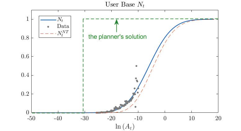
24Figure 5: User Subsidy vs. Token. This figure plots Nt for the tokenized economy (blue solid curve),
the tokenless economy (red dotted curve), and the tokenless economy with subsidy κ = 0.5φ (green dash
curve).
6 Extensions and Discussions
6.1 Subsidy as an Alternative Solution to User Adoption
In this subsection, we compare tokens with a traditional alternative solution to network
adoption – user subsidy (Rochet and Tirole, 2006) – and discuss the associated technical
and financial considerations that affect the implementation.
Let κ denote the lump-sum subsidy that the platform gives to a user for platform par-
ticipation per unit of time. Given this subsidy, agent i solves the following problem at each
t:
dyi,t = max 0, max [κdt + dvi,t ] , (44)
xi,t >0
where dvi,t is given in (2). Without this subsidy, this objective function is the same as (2)
in the tokenless economy. By combining the subsidy κ with the participation cost φ, we can
equivalently interpret introducing κ as reducing the participation cost from φ to φ − κ.
Panel A of Figure 5 compares the adoption dynamics of token-based economy (the solid
blue curve), the tokenless economy (the dotted red curve), and the tokenless economy with
subsidy κ = 0.5φ (the dash green curve). Here we allow a sufficiently generous subsidy that
25effectively reduces agents’ cost of participation by half. In this case, subsidy lifts up the
adoption curve, but it is still below what tokens can achieve.
Charging fees on profits. One question remains: How to finance the subsidies paid to
users? Subsidies are often made possible by charging fees to users. One way to introduce
fees in our analysis is via a standard proportional tax, τt , which can be time-varying and
state-dependent. Given τt , agent i solves the following modified problem:
1−α ui α
dyi,t = max 0, (1 − τt ) max (xi,t ) (Nt At e ) dt − (φ − κ)dt − xi,t rdt . (45)
xi,t
As the fee is charged on the maximized profit, introducing τt does not affect agent i’s choice
of xi,t and adoption decision.23
The fee charged on users, τt > 0, can be set to finance the subsidy:
Z
τt max κdt + (xi,t )1−α (Nt At eui )α dt − φdt − xi,t rdt dG (ui ) = κNt dt, (46)
ui ≥ut xi,t >0
where the left side gives the total fees collected from users and the right side is the total
subsidy to users. For τi to be feasible, it has to be smaller than 100%. In the early stage
where At is sufficiently low, the τt implied by the subsidy can be greater than 100% and thus
infeasible. In contrast, tokens do not have this problem. The adoption-accelerating effect is
active even when At is extremely low. In fact, as show by Panel B of Figure 3, the expected
token return, µPt , is larger when At and Nt are smaller, and thereby, the future potential of
adoption, i.e., 100% − Nt , is larger. This is one advantage of tokens over subsidies.
Second, implementing this tax-subsidy scheme can be more difficult than tokens. Agents
may not truthfully report their profits from platform activities because agents’ type, ui , can
be private information. Incomplete information is a classic challenge recognized by stud-
ies on optimal taxation in the public finance literature (e.g., Mirrlees, 1971). Moreover, our
analysis assumes that agents receive subsidy only if they participate. If agents can obtain the
subsidy and fake participation, the subsidy becomes a pure outflow of the platform and does
23
If the maximized profit is positive when τt = 0, it is still positive when τt ∈ (0, 1) and agent i still
participates. This result resembles the standard result that a firm is neutral to profit taxes.
26You can also read