Global cotton production under climate change - Implications for yield and water consumption - HESS
←
→
Page content transcription
If your browser does not render page correctly, please read the page content below
Hydrol. Earth Syst. Sci., 25, 2027–2044, 2021
https://doi.org/10.5194/hess-25-2027-2021
© Author(s) 2021. This work is distributed under
the Creative Commons Attribution 4.0 License.

Global cotton production under climate change – Implications for
yield and water consumption
Yvonne Jans1,2 , Werner von Bloh1 , Sibyll Schaphoff1 , and Christoph Müller1
1 Potsdam Institute for Climate Impact Research, Member of the Leibniz Association,
P.O. Box 60 12 03, 14412 Potsdam, Germany
2 Department of Geography, Humboldt-Universität zu Berlin, Unter den Linden 6, 10099 Berlin, Germany

Correspondence: Yvonne Jans (jans@pik-potsdam.de)

Received: 7 November 2019 – Discussion started: 16 January 2020
Revised: 28 February 2021 – Accepted: 4 March 2021 – Published: 16 April 2021

Abstract. Being an extensively produced natural fiber on         scenarios in less VWC compared to ambient CO2 conditions.
earth, cotton is of importance for economies. Although the       Under RCP6.0 and RCP8.5, VWC is notably decreased by
plant is broadly adapted to varying environments, the growth     more than 2000 m3 t−1 in areas where cotton is produced un-
of and irrigation water demand on cotton may be challenged       der purely rainfed conditions. By 2040, the average global
by future climate change. To study the impacts of climate        VWC for cotton declines in all scenarios from currently
change on cotton productivity in different regions across the    3300 to 3000 m3 t−1 , and reduction continues by up to 30 %
world and the irrigation water requirements related to it, we    in 2100 under RCP8.5. While the VWC decreases by the
use the process-based, spatially detailed biosphere and hy-      CO2 effect, elevated temperature acts in the opposite direc-
drology model LPJmL (Lund–Potsdam–Jena managed land).            tion. Ignoring beneficial CO2 effects, global VWC of cotton
We find our modeled cotton yield levels in good agreement        would increase for all RCPs except RCP2.6, reaching more
with reported values and simulated water consumption of          than 5000 m3 t−1 by the end of the simulation period under
cotton production similar to published estimates. Follow-        RCP8.5. Given the economic relevance of cotton production,
ing the Inter-Sectoral Impact Model Intercomparison Project      climate change poses an additional stress and deserves spe-
(ISIMIP) protocol, we employ an ensemble of five general         cial attention. Changes in VWC and water demands for cot-
circulation models under four representative concentration       ton production are of special importance, as cotton produc-
pathways (RCPs) for the 2011–2099 period to simulate fu-         tion is known for its intense water consumption. The impli-
ture cotton yields. We find that irrigated cotton production     cations of climate impacts on cotton production on the one
does not suffer from climate change if CO2 effects are con-      hand and the impact of cotton production on water resources
sidered, whereas rainfed production is more sensitive to vary-   on the other hand illustrate the need to assess how future cli-
ing climate conditions. Considering the overall effect of a      mate change may affect cotton production and its resource
changing climate and CO2 fertilization, cotton production on     requirements. Our results should be regarded as optimistic,
current cropland steadily increases for most of the RCPs.        because of high uncertainty with respect to CO2 fertilization
Starting from ∼ 65 million tonnes in 2010, cotton produc-        and the lack of implementing processes of boll abscission un-
tion for RCP4.5 and RCP6.0 equates to 83 and 92 mil-             der heat stress. Still, the inclusion of cotton in LPJmL allows
lion tonnes at the end of the century, respectively. Under       for various large-scale studies to assess impacts of climate
RCP8.5, simulated global cotton production rises by more         change on hydrological factors and the implications for agri-
than 50 % by 2099. Taking only climate change into ac-           cultural production and carbon sequestration.
count, projected cotton production considerably shrinks in
most scenarios, by up to one-third or 43 million tonnes un-
der RCP8.5. The simulation of future virtual water content
(VWC) of cotton grown under elevated CO2 results for all

Published by Copernicus Publications on behalf of the European Geosciences Union.
2028                                                                   Y. Jans et al.: Cotton production under climate change

1   Introduction                                                   version 4.0 (Schaphoff et al., 2018b). We provide an eval-
                                                                   uation of model skill by comparing simulated cotton yields
Being an extensively produced natural fiber on earth, cotton       to yield statistics (FAO, 2018). To study climate change im-
(Gossypium spp.) is providing income to millions of farm-          pacts on future cotton productivity, we simulate future cot-
ers. According to the World Bank Atlas (Sheth, 2017), 8            ton yields and related irrigation water requirements under a
of the top 10 cotton-producing countries are classified as         set of future climate scenarios (Hempel et al., 2013), follow-
developing countries, and their exports of the crop reached        ing the Inter-Sectoral Impact Model Intercomparison Project
∼ USD 30 billion in 2017 (ITC, 2019) (full overview in Ta-         (ISIMIP) protocol (Warszawski et al., 2014).
ble S1). Particularly in the West African region – the world’s
third-largest cotton exporter (following North America and
Central Asia) – cotton has played an important part in the         2     Materials and methods
economic development and has remained a key source of
livelihood for many farmers (Hussein et al., 2005; Perret          2.1    The LPJmL model
and Bossard, 2006). Worldwide, cotton is already broadly
adapted to growing in temperate, subtropical, and tropical         The global dynamic vegetation model LPJmL is a well-
environments, but growth may be challenged by future cli-          established and thoroughly evaluated model (Schaphoff
mate change (Bange et al., 2016). Climate change is likely to      et al., 2018b, a; Müller et al., 2017) that is unique in combin-
affect cotton production both positively and negatively. Tem-      ing natural vegetation, hydrology, and managed ecosystems
perature influences cotton growth and development by deter-        (croplands, pastures) in one consistent framework for grid-
mining rates of fruit production, photosynthesis, and respira-     ded large-scale applications. The model has been extensively
tion (Turner et al., 1986; Hearn and Constable, 1984).             described by Schaphoff et al. (2018b), and we here only
   However, the growth of cotton plants differs at varying         provide a short summary of the most relevant features for
stages of plant development and by plant organ (Burke and          this study and the extensions implemented for cotton. Agri-
Wanjura, 2010), and thus a temperature optimum for cotton          cultural crops have been implemented as annual crops with
cannot be defined. Yield and growth of cotton are directly         daily computation of photosynthesis, autotrophic respiration,
affected by a high temperature. Additionally, hot weather          evapotranspiration, and allocation of assimilates to plant or-
conditions increase the evaporative demand on cotton plants,       gans (Bondeau et al., 2007). Individual crops are grown on
leading to more intense water stress (Hall, 2000). Elevated        separate spatial units (stands) within each grid cell so that
atmospheric carbon dioxide concentrations ([CO2 ]) on the          different crops do not compete for water and light, mimick-
other hand are expected to increase cotton yields as cotton is     ing monocultures. Also purely rainfed and irrigated crop cul-
a C3 crop (Kimball, 2016). Numerous free-air carbon diox-          tivation can be simulated on separate stands, and irrigation
ide enrichment (FACE) studies demonstrated a strong reac-          water can be applied by different irrigation techniques and
tion of cotton yield and growth to an increased CO2 con-           can be limited by actual freshwater availability (Jägermeyr
centration (Kimball, 1983; Cure and Acock, 1986; Hileman           et al., 2015). LPJmL – here operated at a 0.5 arcdeg spatial
et al., 1994; Hendrix et al., 1994; Reddy et al., 1997; Mauney     resolution – simulates processes underlying the growth and
et al., 1994; Bhattacharya et al., 1994). Likewise, water-         productivity of both natural and agricultural vegetation (Sitch
use efficiency can be improved by CO2 enrichment because           et al., 2003; Bondeau et al., 2007; Lapola et al., 2010; Rolin-
it increases biomass and causes partial stomatal closure at        ski et al., 2017). The model represents 10 plant functional
the same time, consequently reducing transpiration (Mauney         types (PFTs) as well as 12 crop functional types (CFTs) and
et al., 1994; Hileman et al., 1994; Broughton, 2015; Ko and        3 bioenergy plantation systems (Beringer et al., 2011). In
Piccinni, 2009).                                                   LPJmL, carbon, water, and energy fluxes are closely linked
   Crop models have been used to assess the effect of chang-       to reproduce plant growth dynamics and to account for the
ing climate conditions on crop productivity, but the main fo-      effects of changes in climate conditions and water availabil-
cus has been on major staple crops – such as maize, wheat,         ity (Gerten et al., 2004, 2007). Several features – such as
rice, and soybean (e.g., Challinor et al., 2014; Rosenzweig        river routing (Rost et al., 2008a), irrigation systems (Jäger-
et al., 2014; Müller et al., 2015; Pugh et al., 2016; Schleuss-    meyr et al., 2015), a soil hydrological and carbon distribution
ner et al., 2018) – that provide the majority of calories to hu-   scheme (Schaphoff et al., 2013), and a fire module (Thonicke
man nutrition (Yahia et al., 2019; Welch and Graham, 2004).        et al., 2010) – further improved the model. The calculation of
   The response of other crops has been assessed less thor-        photosynthesis is based on the Farquhar model (Collatz et al.,
oughly, despite their importance for economies or human            1991; Haxeltine and Prentice, 1996; Sitch et al., 2003). Water
nutrition. With this study, we aim to examine the impacts          consumption is ruled by plant physiology, and the coupling
of climate change on cotton productivity in different regions      between vegetation and water cycle enables the separation
across the world. We therefore add cotton as an additional         of productive (transpiration) and unproductive (interception,
crop to the global dynamic vegetation, hydrology, and crop         evaporation) portions of plant water use. Moreover, water
growth model LPJmL (Lund-Potsdam-Jena managed land)                flows are divided into green (precipitation) and blue (irriga-

Hydrol. Earth Syst. Sci., 25, 2027–2044, 2021                                       https://doi.org/10.5194/hess-25-2027-2021
Y. Jans et al.: Cotton production under climate change                                                                          2029

tion) water (Rost et al., 2008b; Jägermeyr et al., 2015, 2016).      ing. Crop maturity is characterized by slowed development
The evaluation of various model components – e.g., crop              of new main-stem nodes, causing first-position white flowers
yields, evapotranspiration, and river discharge – has shown          to appear progressively closer to the plant apex (Oosterhuis
that LPJmL is a tool suitable for analyzing changes in vege-         et al., 1993). The development of cotton plants is particu-
tation and water. Schaphoff et al. (2018a) provide a compre-         larly sensitive to temperature, leading to an acceleration of
hensive evaluation of the LPJmL model.                               all stages of phenological development (Bange et al., 2001;
                                                                     Hodges et al., 1993; Reddy et al., 1997). However, being an
2.2     Implementation and parameterization of cotton                indeterminate plant, the phenological phases of cotton can-
                                                                     not be clearly distinguished and represented as a function of
Twelve crop types are already implemented in LPJmL (tem-             temperature (Bange et al., 2016), and the growing period is
perate and tropical cereals, pulses, maize, rice, temperate          thus not necessarily shortened by warming as, e.g., observed
and tropical roots, sunflower, soybeans, groundnut, rapeseed,        in annual crops.
sugar cane) (Bondeau et al., 2007; Lapola et al., 2010). In this        To account for the current production system, cotton is
study we include cotton, which was originally implemented            implemented in LPJmL as small agricultural trees that are
as a perennial crop in LPJmL by Fader et al. (2015) for the          planted annually and removed at the end of the growing pe-
Mediterranean region. However, in most parts of the world,           riod, representing the annual production mode.
cotton is cultivated as an annual crop (Ritchie et al., 2007;           The phenology – i.e., the temporal dynamic of the canopy
Whitaker et al., 2018). We modify the modeling approach              greenness – is computed with the growing season index con-
developed by Fader et al. (2015) accordingly and implement           cept as described and parameterized by Forkel et al. (2014).
cotton into LPJmL version 4.0 (Schaphoff et al., 2018b) as an        The daily phenology status is determined by multiplying lim-
annual crop. Similar to Fader et al. (2015), the cotton plant        iting effects of cold temperature, short-wave radiation, wa-
is simulated and parameterized as an agricultural tree, and          ter availability, and heat stress. Thus, vegetation greenness
we calculate phenology and growth on a daily basis (see be-          is limited by temperature-induced heat stress. The saplings
low). We adopt most of the key parameters used by Fader              are initialized with 2.3 gC of sapwood and a leaf-area index
et al. (2015) and adjust values for plant density and temper-        of 1.6 m2 m−2 . Similar to phenology, gross primary produc-
ature optimum for photosynthesis (Table 1). Other than ad-           tion (GPP) and net assimilation (NPP) of cotton plants are
justing these two parameters, we did not calibrate any plant         calculated daily. Increasing daily air temperature values lead
growth parameters. To account for regional differences, we           to a higher respiration (maintenance) rate, which can exceed
use country-specific planting densities provided by several          carbon assimilation, resulting in a negative NPP (Schaphoff
studies (Sect. 2.2.2). As the intensity of irrigation on irrigated   et al., 2018b). Fruit growth is expressed as daily carbon ac-
cotton-producing areas in the different production regions is        cumulation (Cfruit ) of a fraction of NPP after square set, i.e.,
unknown, we conduct simulations with different levels of             as soon as squares (pre-bloom fruiting buds) emerge. The
deficit irrigation (25, 50, 75, and 100 % of required irriga-        development of squares indicates the initiation of a fruit-
tion water) and select the irrigation level that produces the        ing branch. The model implementation assumes that cotton
cotton yield that is closest to observations (Sect. 2.3). In this    fruit growth occurs after the fractional cover of green leaves
study, simulated cotton yields should be understood as the           has reached 60 % of full leaf cover, i.e., when the phenol-
entire cotton fruit, that is, both cotton lint and cottonseed.       ogy scaler phen = 0.6. This follows the description of Ritchie
                                                                     et al. (2007) on the canopy and fruit development of cotton
2.2.1    Phenology and growth                                        plants.

Wild cotton is a deciduous perennial tree, and the fruiting          Cfruit = max(0, NPP) × HR,                                   (1)
habit of the plant is not clearly established; i.e., vegetative
and reproductive growth occur at the same time (Ritchie              where HR is the harvest ratio and NPP the daily net pri-
et al., 2007). During the growing period the leaves sup-             mary productivity of the tree. On days with negative NPP,
ply photosynthates to plant growth and the developing fruit          fruit growth is halted, but accumulated yield is not reduced,
and are shed only when the plant is stressed such as during          reflecting the fact that boll development dominates plant
drought, disease, nutrient starvation, or frost (Wullschleger        growth at this stage of reproductive growth (Ritchie et al.,
and Oosterhuis, 1990). The perennial nature of cotton, even          2007). At the end of the growing period, cotton harvest H is
its modern cultivars, is not helpful in achieving high yields        determined as
of cotton lint and seed. Consequently, through breeding and               DH
changes in cultivation practices, cotton is now farmed as an
                                                                          X
                                                                     H=         Cfruit ,                                          (2)
annual crop to prevent diseases and optimize cotton produc-                DS
tion (Ritchie et al., 2007; Whitaker et al., 2018). Once the
entire crop is mature, the leaves serve no useful purpose,           where the day of square set (DS ) and harvest day (DH ) define
and their removal can be beneficial for mechanical harvest-          the length of the simulated reproductive period.

https://doi.org/10.5194/hess-25-2027-2021                                           Hydrol. Earth Syst. Sci., 25, 2027–2044, 2021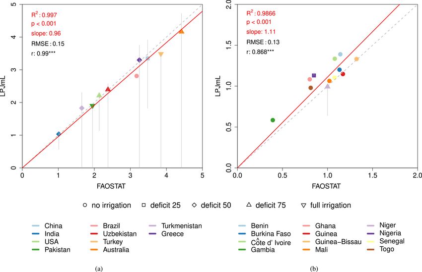
2030                                                                                            Y. Jans et al.: Cotton production under climate change

Table 1. Key parameters of cotton according to Fader et al. (2015).

        Crop       Seasonality                        Kest (trees ha−1 )         HR (frac)        Tb (◦ C)       Phopt (◦ C)         Tlim (◦ C)      WCF (% of DM)
        Cotton     Deciduous broadleaved              30 000–100 000∗                   0.19              15       16 to 32∗        −10 to 40                       91
    Values marked with an asterisk (∗ ) were adjusted. Kest : tree density range; HR: harvest ratio; Tb : base temperature; Phopt : optimum temperature range for
    photosynthesis; Tlim : lower and upper coldest monthly mean temperature; WCF: conversion factor (moisture content) from dry to fresh matter.

    A possible simultaneous establishment of herbaceous                                     and water stress can still affect interannual yield variability
PFTs in the same areas of agricultural trees, representing                                  in irrigated systems. In order to test the importance of deficit
grasses and weeds (for modeling details see Schaphoff et al.,                               irrigation for cotton production, we performed several runs,
2018b), can be simulated by LPJmL but was turned off in                                     varying the fraction of soil pore space filled up in individ-
the simulations here. This mimics effective weed control,                                   ual irrigation events from 0 (corresponding to purely rainfed
mainly practiced in cotton farming today to reduce compe-                                   conditions) to 1 (meeting full irrigation demand) by incre-
tition for water and nutrients (Ritchie et al., 2007; Whitaker                              ments of 0.25.
et al., 2018).                                                                                 If the soil water content in the upper 50 cm of the soil falls
                                                                                            below 90 % of field capacity, an irrigation event is triggered.
2.2.2    Specification of planting densities, sowing dates,                                 Soil water lower than atmospheric water demand requires a
         and irrigation                                                                     daily net irrigation (NIR, millimeters). NIR is calculated as
                                                                                            the amount of water needed to fill soil water up to field ca-
A country-specific planting density (kest ) is used as model                                pacity Wfc in the upper root layers of the soil.
input, which is, apart from irrigation and sowing dates, the
only management aspect that is explicitly considered. These                                 NIR = max(0, (Wfc − wa )),                                                   (3)
country-specific planting densities have been taken from the
literature (Abdullaev et al., 2007; Iqbal et al., 2012; Venu-                               where wa is the soil water in millimeters actually available.
gopalan et al., 2013; Dong et al., 2006; Bednarz et al., 2006;                                 Inefficiencies of different irrigation systems cause addi-
Zhi et al., 2016; Khan et al., 2017; Bozbek et al., 2006; Echer                             tional water needs to meet crop water demand. For that rea-
and Rosolem, 2015; Dai and Dong, 2014; Vaughan, 2005;                                       son, LPJmL considers conveyance efficiency (Ec ) and calcu-
Akhtar et al., 2002) and are shown in Fig. S1. The cotton-                                  lates application requirements (AR) for each system. Conse-
specific planting density parameter (plants m−2 a−1 ) was in-                               quently, the gross irrigation requirement (GIR; millimeters)
troduced similar to the annual establishment rate kest of PFT                               – i.e., the amount of water requested for abstraction – results
individuals (Schaphoff et al., 2018b).                                                      in
   The growing season of cotton plants is prescribed from                                               NIR + AR − Store
the sources specified in Sect. 2.3. Thereby the sowing date                                 GIR =                        ,                                               (4)
                                                                                                              Ec
defines the start of the growing period and ranges between
Julian day 1 and 335 of the year of sowing. The prescribed                                  where Store is a storage buffer. The storage buffer is filled
growing season length varies from 153 to 243 d for cotton                                   up with available irrigation water not used due to available
plants to reach harvest.                                                                    precipitation and is released in the next irrigation event. A
   Five hydrologically and thermally active layers represent                                detailed explanation about the computation of NIR, GIR, and
the soil profile in LPJmL where roots access water, depend-                                 Store in LPJmL is given in Rost et al. (2008b) and Jägermeyr
ing on their PFT/CFT-specific root distribution (Schaphoff                                  et al. (2015). The application requirements are calculated as
et al., 2018b). The soil water content of the first layer deter-                            AR = max(0, (Wsat − Wfc ) × DU − wfw ,                                       (5)
mines the infiltration rate, and water not infiltrated forms the
surface runoff. Similar to the infiltration approach, the per-                              where Wsat is the soil moisture content at saturation level (in
colation rate is limited by soil moisture of the lower layer,                               mm); DU is an irrigation system-specific scalar (no unit), to
and excess water above saturation feeds the lateral runoff                                  distribute irrigation water uniformly across the field, and wfw
(Schaphoff et al., 2013).                                                                   is the available free water (in millimeters) (Jägermeyr et al.,
   Cotton is produced in rainfed or irrigated systems, whereas                              2015). Note that the computation of GIR is relevant for sim-
irrigation generally serves to reduce the impacts of rainfall                               ulations in which irrigation water is constrained by available
deficits and thus reduces interannual yield variability. How-                               river discharge and reservoir capacity (e.g., Jägermeyr et al.,
ever, the actual amount of water applied to fields is unknown                               2015) but not here, where we assume explicit levels of deficit
and determined by water availability, water management sys-                                 irrigation but no additional constraints on water limitation.
tems, and economic rationale. The extent to which rainfall                                     This model development is based on LPJmL4, a model
deficits are compensated for by irrigation is thus not only a                               version that does not account for nutrient limitations, and,
question of equipment for irrigation (Portmann et al., 2010),                               thus, fertilizer effects are not considered.

Hydrol. Earth Syst. Sci., 25, 2027–2044, 2021                                                                       https://doi.org/10.5194/hess-25-2027-2021
Y. Jans et al.: Cotton production under climate change 2031
2.3 Modeling protocol, input, and reference data Cotton yield levels modeled under different irrigation op-
tions on irrigated cotton areas (Sect. 2.2.2) were compared
with national yield levels published by FAO (2018), reported
All simulations are conducted at a 0.5◦ longitude–latitude as “Seed cotton” there. Since LPJmL is a global model, we
grid resolution with daily weather input data and annual data evaluated the model at the global and national level. How-
on atmospheric carbon dioxide concentrations ([CO2 ]). To ever, on the grid cell level simulated cotton yield results
simulate historical results, we ran the LPJmL model for the were also tested against semi-controlled field experiments.
period 1901–2011 using the Climate Research Unit’s TS 3.23 For these comparisons management assumptions (sowing
monthly data for temperature, wet days, and cloudiness (Har- and harvest dates, planting densities) were adapted to repro-
ris et al., 2014) and precipitation data (Version 5) provided by duce experimental conditions (Fig. S8).
the Global Precipitation Climatology Centre (Rudolf et al.,
2011). Monthly weather input data are converted to daily
data, using an internal weather generator (Schaphoff et al., 3 Results
2018b). Data on [CO2 ] refer to records at the Mauna Loa
station (Tans and Keeling, 2015). A 120-year spin-up (recy- 3.1 Evaluation of model performance
cling the first 30 years of input climatology) preceded tran-
sient runs to bring water fluxes and soil temperatures into dy- In order to evaluate the performance of this extended LPJmL
namic equilibria. As soil carbon pools have no effect on cot- model version, simulated historical cotton yields are com-
ton productivity in this version of the model, a longer spin- pared to observed data (Fig. 1) published by FAOSTAT
up to correctly initialize soil and vegetation carbon pools (FAO, 2018). The modeled cotton yield levels are in good
(Schaphoff et al., 2018b) is not necessary here. Simulations agreement with reported values. Statistical analyses for both
for future periods are conducted for four different represen- the top 10 cotton-producing countries and cotton-growing
tative concentration pathways (RCPs) – RCP2.6, RCP4.5, countries in West Africa show that simulated national yield
RCP6.0, and RCP8.5 (Moss et al., 2010) – each imple- levels can reproduce reported national yield levels well
mented by five different general circulation models (GCMs): (Fig. 1). For the top 10 cotton-producing countries, cotton
GFDL-ESM2M (Dunne et al., 2012, 2013), HadGEM2-ES yields simulated under full irrigation often match FAO val-
(Jones et al., 2011), IPSLCM5A-LR (Dufresne et al., 2013), ues best. The whiskers that depict the range of yield levels
MIROC-ESM (Watanabe et al., 2011), and NorESM1-M simulated with different irrigation options on the irrigated
(Bentsen et al., 2013), which have been bias-corrected as de- cotton cropland often reach the zero line, indicating that cot-
scribed by Hempel et al. (2013). Data on [CO2 ] for future pe- ton production in these countries (Pakistan, Turkmenistan,
riods are taken from the corresponding RCP data sets (Moss Turkey, Uzbekistan, etc.) is not possible without irrigation.
et al., 2010) as provided by the ISIMIP project (Frieler et al., National yield levels can also be reproduced well in West
2017). To assess how cotton plants respond to future climate Africa, where in contrast to the top 10 producer countries
change, we ran the model for the time span 1951–2099, again hardly any irrigated cotton production exists (Fig. S2). An
preceded by a 120-year spin-up period. The averaging time overview of the model performance for all cotton-growing
for historical yields differs (depending on the purpose) and countries is given in the Supplement, Table S2.
is indicated for each figure. Future yield projections are pre- For these simulations, the planting densities in LPJmL
sented as 2070–2099 averages, compared to annual means have not been calibrated against observed yield levels but are
averaged over the reference period 1980–2009, or as full time based on reported planting densities (Fig. S1). The model
series. The spatial distribution of cropland dedicated to cot- simulations can reproduce statistically significant shares of
ton was taken from the land-use data set MIRCA2000 (Port- reported variability in time of intensely managed top produc-
mann et al., 2010), which provides both rainfed and irrigated ing countries, such as the USA and Australia as well as a few
harvested areas around the year 2000 with a spacial resolu- West African countries (Figs. 2 and S4) and other countries
tion of 5 arcmin (Fig. S2). (Table S2). The model also reproduces some of the histori-
Sowing dates and growing period were provided as grid- cal interannual variation in global cotton production (Fig. 3).
ded model input, combining sowing and harvest informa- The spatial pattern of cotton yields is shown in Fig. S5.
tion provided by the ICAC’s World Cotton Calendar (WCC) We further evaluate the model results with respect to the
(Committee, 2014) and Portmann et al. (2010). More pre- water consumption of cotton production against data pro-
cisely, we used the WCC data and filled gaps with data of- vided by Chapagain et al. (2006), averaged over the time
fered by MRICA (Fig. S3). Because increasing temperatures period 1997–2001. For reasons of comparability, we there-
do not necessarily shorten the period of growth for cotton fore followed the concept of “virtual water content” (Allan,
plants (Bange et al., 2010; Luo et al., 2014a) and parame- 1997, 1998) and calculated the virtual water content of cot-
terization of cotton partly reflects more advanced cultivars ton (tonnes per meter) as the ratio of the water (green and
(Sect. 2.2), we here assume that the growing season length blue in cubic meters per hectare) used to grow a crop in
remains static in all simulations. the field to the related crop yield (tonnes per hectare). We
https://doi.org/10.5194/hess-25-2027-2021 Hydrol. Earth Syst. Sci., 25, 2027–2044, 20212032 Y. Jans et al.: Cotton production under climate change
Figure 1. Comparing simulated cotton yields [t ha−1 ] to observed values for (a) the top 10 cotton-producing countries and (b) West African
countries. Whiskers indicate the yield range of different irrigation options on irrigated cotton cropland in these countries (Portmann et al.,
2010). LPJmL yield data and FAOSTAT yield data were both averaged over the time period 2000–2009.
find that LPJmL simulations of water consumption of cot- For the evaluation of the modeled cotton yield response to
ton production are in good agreement with the estimates of elevated [CO2 ], we compare simulated yield effects to those
Chapagain et al. (2006) with respect to the order of magni- reported from open-top chamber (OTC) and FACE experi-
tude and spatial variability (Fig. S6 and Table 2). The virtual ments. Kimball (2016) report strong yield increases in cot-
water content is quite variable across regions and mainly in ton bolls under elevated [CO2 ] (∼ 38 %), which is a stronger
an inverse relation of the yield pattern (Fig. S5), suggesting yield response than most other crops. Experimental data from
that spatial yield variability is higher than the spatial vari- Kimball et al. (1992) and Mauney et al. (1994) also show that
ability in actual evapotranspiration. As virtual water content the level of water and nutrient availability affects the relative
is a criterion for water-use efficiency (Hoekstra, 2003; Hoek- cotton yield response to elevated [CO2 ]. Similarly, LPJmL
stra and Mekonnen, 2012; Zhuo and Hoekstra, 2017), mod- yields also result in a strong response depending on the level
erate values in regions with high irrigation shares (compare of [CO2 ] increase and water stress (see Fig. S8). Observa-
Figs. S6 and S7) point to an efficient use of (blue) water. The tional data are only available for one OTC site (Phoenix,
efficiency of blue-water use depends on management prac- AZ, USA) and one FACE site (Maricopa, AZ, USA), so it
tices – such as irrigation techniques, irrigation strategies, and remains unclear how the cotton yield response to elevated
mulching practices (Gleick, 2003; Perry, 2007; Perry et al., [CO2 ] varies across different climate zones and management
2009; Zhuo and Hoekstra, 2017) – to reduce non-beneficial regimes. However, the range of simulated yield increases un-
losses (soil evaporation) as well as on other yield-reducing der elevated [CO2 ] seems to be often adequately reproduced
factors, such as nutrient limitations or pests. In the Indo- by LPJmL in the corresponding grid cells (Fig. S8).
Gangetic plain, drip irrigation of cotton is only applied in
experimental fields, and farmers grow cotton by applying ir- 3.2 Climate change impacts on cotton production
rigation water through flood irrigation (Thind et al., 2008;
Aujla et al., 2008). Here, the water consumption of cotton Considering the overall effect of climate change and CO2
production is at the high end, indicating substantial non- fertilization, future cotton productivity slightly increases –
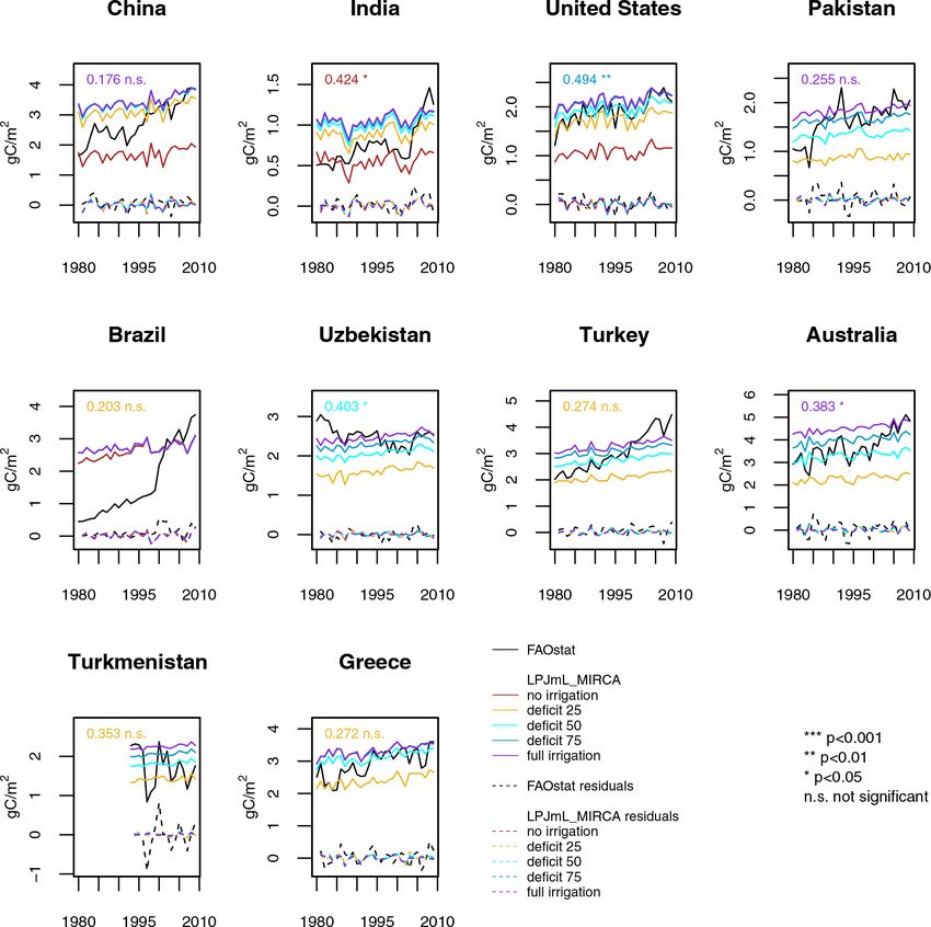
beneficial water losses (Thind et al., 2010). starting from ∼ 65 million tonnes in 2010 – until 2040
for all RCPs similarly by ∼ 10 %. For RCP2.6, global cot-
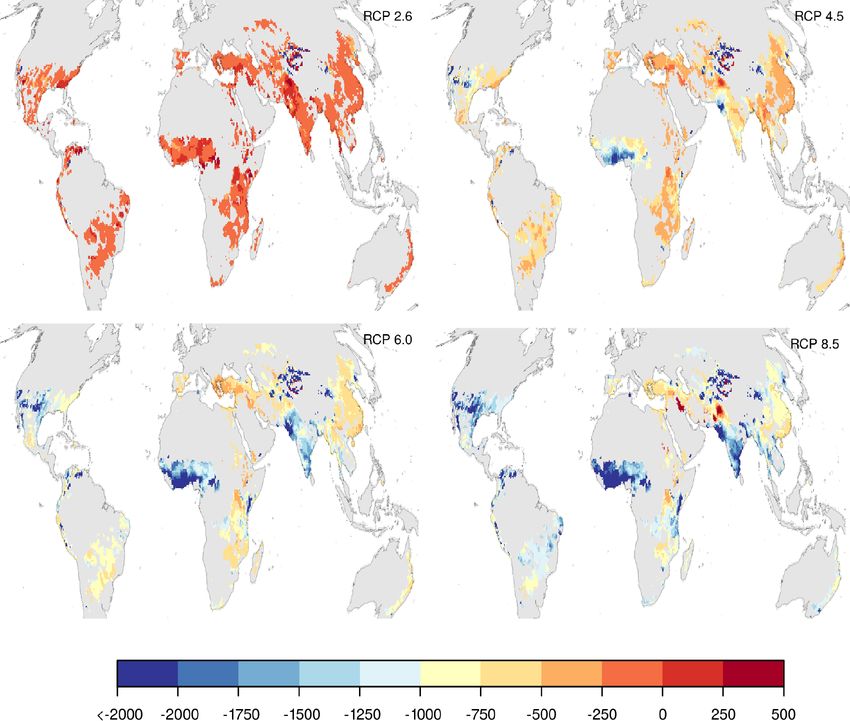
Hydrol. Earth Syst. Sci., 25, 2027–2044, 2021 https://doi.org/10.5194/hess-25-2027-2021Y. Jans et al.: Cotton production under climate change 2033 Figure 2. Comparing interannual yield variability for the top 10 cotton-producing countries. Numbers in each plot depict the correlation coefficient between simulated residuals and FAOSTAT residual data. The different irrigation options (on irrigated cropland only) are shown in colored lines. The color of the correlation coefficient indicates the best-fitting irrigation option. For Turkmenistan, yields have only been reported from 1992 onward (FAO, 2018), so only these years are shown in the plot. ton production on current cropland slightly declines after spatial patterns of projected yield increases seem to be quite 2040, while for the remaining RCPs simulated production static but scale with the emission scenario (RCP, Fig. S10). on current cropland steadily increases. Looking at RCP4.5 The projected increases in yield are the result of interact- and RCP6.0, cotton production equates to 83 and 92 mil- ing processes, which are often dominated by a positive re- lion tonnes at the end of the century, respectively. Under sponse to elevated [CO2 ]. Higher temperatures initially stim- RCP8.5, simulated global cotton production rises by more ulate cotton plant growth by accelerating phenological pro- than 50 % up to 102 million tonnes by 2099 (Figs. 4 and S9 cesses and thus reaching full canopy closure earlier in the for relative changes). season. If, however, high temperatures persist throughout the Spatial patterns of projected changes in cotton yields growing season, phases of plant stress (heat and water stress) (Fig. S10) show that increases are mainly expected in cooler emerge earlier and then reduce leaf cover and halt the re- or irrigated environments (Fig. S2), but exceptions exist, such productive growth of cotton plants. This yield-decreasing as Pakistan and northern India, where cotton yields are pro- effect of climate change is masked by the strong growth- jected to only slightly increase despite irrigation. Overall, the stimulating effect of elevated [CO2 ] (see Figs. S11 and S12 https://doi.org/10.5194/hess-25-2027-2021 Hydrol. Earth Syst. Sci., 25, 2027–2044, 2021
2034                                                                        Y. Jans et al.: Cotton production under climate change

Figure 3. Time series of historical global cotton production [million tonnes per year]. The number in the plot depicts the correlation coeffi-
cient between simulated residuals and FAOSTAT residuals.

Table 2. Virtual water content and consumptive water use for cotton production in the major cotton-producing countries for the period 1997–
2001. Reference data taken from Chapagain et al. (2006), here referred to as C06. VWCblue : blue virtual water content; VWCtotal : total
virtual water content; Airrig : irrigated harvested cotton area; Atotal : total harvested cotton area.

                      Virtual water content [m3 t−1 ]                                                        Consumptive water use [mm]
                          Total              Blue          VWCblue / VWCtotal        Airrig / Atotal           Total             Blue
                    LPJmL         C06    LPJmL      C06    LPJmL            C06     LPJmL       C06        LPJmL       C06   LPJmL       C06
 Argentina             2564       7700     142      2307      0.06          0.30       0.08        1         775     877        43        263
 Australia             2536       2278    1677      1408      0.66          0.62          1      0.9        1177     843       778        521
 Brazil                3235       2621      20        46      0.01          0.02       0.02     0.15         895     551         5         10
 China                 1907       2018     481       760      0.25          0.38       0.41     0.75         716     638       180        240
 Egypt                 2727       4231    2605      4231      0.96          1.00          1        1         963   1009        921      1,009
 Greece                2554       2338    1586      1808      0.62          0.77          1        1         937     707       582        547
 India                 5232       8662    1773      2150      0.34          0.25       0.36     0.33         563     538       191        134
 Mali                  5738       5218       0      1468      0.00          0.28          0     0.25         594     538         0        151
 Mexico                4191       2508    2538      1655      0.61          0.66       0.97     0.95         933     746       565        492
 Pakistan              5486       4914    4377      3860      0.80          0.79          1        1        1033     850       824        668
 Syria                 2689       3339    2005      3252      0.75          0.97          1        1        1008   1,309       751      1,275
 Turkey                2779       3100    1796      2812      0.65          0.91          1        1         943     963       609        874
 Turkmenistan          4076       6010    3538      5602      0.87          0.93       0.98        1         926   1025        804        956
 USA                   3461       2249     966       576      0.28          0.26       0.37     0.52         775     419       216        107
 Uzbekistan            3616       4460    2854      4377      0.79          0.98          1        1         911     999       719        981
 Global average        3338       3644    1397      1818      0.42          0.50      0.491            –     755         –     320         –

for simulations with static [CO2 ], where yields continuously            are also projected for the USA, Brazil, India, Pakistan, Cen-
decline with increasing climate change).                                 tral Asia, the southeastern part of China, and Australia if
   Without the beneficial effect of elevated [CO2 ], climate             no effects of CO2 fertilization are assumed. Only for Peru,
change leads to yield declines in most of the current cotton             northeast China, and some parts of Central Asia do the sim-
production area (Fig. S13). Across all RCPs the spatial varia-           ulations project sustained cotton yield gains under climate
tion of impacts shows a diverse pattern, resulting in climate-           change only.
only-induced yield losses up to 2 t ha−1 in large parts of the
cotton production area. Projected cotton yields for the high-
end emission scenario (RCP8.5) decline significantly in Bo-
livia, Argentina, Iraq, Syria, and Egypt. Considerable losses

Hydrol. Earth Syst. Sci., 25, 2027–2044, 2021                                                 https://doi.org/10.5194/hess-25-2027-2021
Y. Jans et al.: Cotton production under climate change 2035
for the CO2 effect leads to an average global virtual water
content of more than 5000 m3 t−1 by the end of the simu-
lation period (Fig. S15a). The spatial pattern reveals that in
all scenarios the virtual water content increases in all regions
if CO2 effects are not accounted for. However, most drastic
changes occur again in West Africa and India, where also
the strongest changes are observed when CO2 effects are ac-
counted for. While the CO2 effect leads to decreasing virtual
water content in these regions, it increases by 2000 m3 t−1 if
the CO2 effects are not accounted for (Fig. S16). Although
cotton production strongly declines if the CO2 effect is ne-
glected, increased VWC values clearly impinge on global
Figure 4. Simulated global cotton production [million tonnes] for water consumption of cotton production. For RCP2.6 and
different RCPs. Transparent colors show the uncertainty ranges of RCP8.5, the evapotranspiration related to cotton plantations
five different GCM patterns. amounts to 244 km3 (3.7 %) and 251 km3 (6.5 %) in 2100,
respectively.
3.3 Climate change impacts on irrigation water
consumption 4 Discussion
While changes in atmospheric CO2 may turn into enhanced 4.1 Model performance
water use or water-use efficiency of cotton production, the
impact of elevated CO2 on cotton growth depends also on The model can reproduce national yield levels very well
plant water availability. The simulation of future virtual wa- (Fig. 1). This can in part be expected as we use the best-
ter content of cotton grown under elevated CO2 results for performing level of deficit irrigation in the comparison as
all scenarios in less virtual water content compared to ambi- well as national planting densities and reported growing sea-
ent CO2 conditions (Fig. 5). While there is only a slight de- sons. However, overall yield levels are often not very sensi-
crease in virtual water content of cotton under RCP2.6, this tive to smaller changes in irrigation levels (full vs. deficit 75),
effect is continuously strengthened across the emission sce- and it is plausible to assume that irrigation typically is ap-
narios (RCPs) for both well-watered and water-stressed con- plied in quantities that are sufficient to eliminate the majority
ditions. Under RCP6.0 and RCP8.5, virtual water content is of water stress. Also, yield levels in countries with no or little
notably decreased by more than 2000 m3 t−1 in areas where irrigation can also be well reproduced. National planting den-
cotton is produced under purely rainfed conditions, e.g., in sities have been taken from literature sources and were not
West Africa and India. By 2040, the average global virtual selected to match observed yield levels. A wide range of (na-
water content for cotton declines in all scenarios from cur- tional) cotton planting densities is reported in the literature,
rently 3300 to 3000 m3 t−1 (Fig. S14a). Thereafter it slightly which would allow for further modification of this parame-
increases again under RCP2.6, while reduction continues for ter to refine our results. However, field research has shown
the remaining scenarios until the end of the century. The most different effects of increasing plant density on cotton yield,
considerable decrease by 30 % results in 2100 under RCP8.5 and to understand how cotton growth is affected by that pa-
(Fig. S14b). The projected reduction of VWC of cotton is rameter multiple interacting factors must be considered (Hei-
predominantly caused by increased cotton productivity, not tholt and Sassenrath-Cole, 2010). In this study, we therefore
by a reduction in cotton water consumption, i.e., the amount have selected planting densities corresponding to the lower
of water evapotranspired in cotton fields. Global cotton wa- end of the spread reported and kept these values static, but
ter consumption slightly increases from currently ∼ 235 km3 the literature suggests that planting densities have changed
by 3.6 and 3 % at the end of the century under RCP2.6 and over time, explaining part of the temporal variation in cotton
RCP8.5, respectively. yields (Venugopalan et al., 2013). Another key component
While the virtual water content improves by the CO2 ef- is the cultivar choice as several breeding programs have de-
fect, elevated temperature (and water stress) acts in the op- veloped high-yielding cotton varieties well adapted to differ-
posite direction. Except for RCP2.6, the global virtual water ent environmental conditions (e.g., Bange and Milroy, 2004;
content of cotton increases slightly but steadily under RCPs Stiller et al., 2004, 2005; Bibi et al., 2008b).
until mid-century. For RCP4.5 and RCP6.0 this development The temporal variation in cotton yields can only partly
continues, resulting in a virtual water content roughly 10 % be reproduced. This comparison is hampered by using static
above the current value by 2100 (Fig. S15b) if no CO2 ef- management assumptions in the absence of good spatially
fect is assumed. The most obvious alteration is projected and temporally resolved management data, which is a gen-
for RCP8.5, where the changing climate without accounting eral difficulty in evaluating gridded crop models’ perfor-
https://doi.org/10.5194/hess-25-2027-2021 Hydrol. Earth Syst. Sci., 25, 2027–2044, 20212036 Y. Jans et al.: Cotton production under climate change Figure 5. Simulated changes in virtual water content of seed cotton [m3 t−1 ] for different RCPs. The spatial pattern of rainfed and irrigated cotton harvested areas was kept constant at the pattern of the year 2000 as provided by Portmann et al. (2010). Gray indicates areas currently not used for cotton production. Values were averaged over the five GCM patterns and over the period 2070–2099. Baseline period for comparison: 1980–2009. mance (Müller et al., 2017). The contribution of weather determine agricultural areas dedicated to cotton (details in variability to yield levels remains unclear as the yield vari- Fader et al., 2015) cause significant deviations from the an- ability in reported yield statistics is affected not only by vari- nual harvested cotton areas provided by FAO (2018), which ability in weather but also by varying management condi- was also reported as a source of uncertainty for other crops tions (Schauberger et al., 2016). Ray et al. (2012) reported (Porwollik et al., 2017). that only 30 % of global yield variability can be attributed The good agreement with Chapagain et al. (2006) on vir- to weather drivers for maize, wheat, rice, and soybean, and tual water content of cotton production adds further trust to Müller et al. (2017) also found better agreement between the model simulations, as productivity and water consump- crop model simulations and yield statistics in high-input tion are intrinsically coupled in the model. Even though the countries, suggesting that agreement between crop model estimates from Chapagain et al. (2006) are also model-based simulations and yield statistics can only be expected in coun- estimates rather than observations, the simulated patterns are tries where management conditions are stable. Larger jumps plausible and have been achieved with different methods. in yield statistics as, e.g., in Brazil, China, India, Pakistan, and several West African countries suggest changes in man- 4.2 Implications of climate impacts agement that cannot be expected to be reproduced by this modeling setup with static management assumptions (Dong Elevated [CO2 ] has been shown to increase leaf photo- et al., 2005; Venugopalan et al., 2013; Rossi et al., 2004). Ad- synthetic rates and crop radiation-use efficiency (Hileman ditionally, inconsistencies between different data sets used to et al., 1994; Idso and Idso, 1994; Reddy and Zhao, 2005; Hydrol. Earth Syst. Sci., 25, 2027–2044, 2021 https://doi.org/10.5194/hess-25-2027-2021
Y. Jans et al.: Cotton production under climate change                                                                          2037

Broughton, 2015) and reduce transpiration at the leaf level       quently, warmer temperatures will increase the rate of plant
through reduced stomatal conductance (Hileman et al., 1994;       development but not necessarily reduce the length of grow-
Broughton, 2015; Zhao et al., 2004) in cotton. Both effects       ing season if temperature seasonality is the limiting factor
potentially lead to improvements in growth and yield. A           (Waha et al., 2012; Minoli et al., 2019) and sufficient water
broad range of yield increases, averaging around 38 %, has        and nutrients are available (Bange and Milroy, 2004; Wang
been reported for cotton bolls for an increase in [CO2 ] of       et al., 2008; Stiller et al., 2004; Luo et al., 2014a; Bange et al.,
190 ppm (360 to 550 ppm), which is substantially stronger         2016). Hence, one major effect that reduces crop yields in
than the average response in most other crops, but only based     annual crops (Ottman et al., 2012; Asseng et al., 2015) is
on a very small set of experiments (Kimball, 2016). In line       not as relevant for cotton. However, cotton management de-
with changes in transpiration rates for canopies under ele-       cisions, such as actively shortening the season for growing
vated [CO2 ], Mauney et al. (1994) reported increased water-      cotton (Constable and Bange, 2015), were not accounted for.
use efficiency as a function of increasing biomass produc-           Climate change is associated with changes in patterns of
tion rather than a reduction in water use in the FACE ex-         precipitation and water availability; hence, cotton plants in
periments. In contrast, Reddy et al. (2005b) showed that in-      some regions may be subjected to plant water deficits. Wa-
creases in temperatures above optimum decrease cotton yield       ter deficit limits growth and productivity of cotton plants,
due to increased boll abscission and smaller boll size. In        and the severity of the problem may increase due to chang-
their experiment, even a significant increase in [CO2 ] did not   ing world climatic trends (Le Houérou, 1996). Plant water
fully compensate for the negative effects on yields. The au-      deficits depend on both the supply of water to the soil and
thors concluded that future increases in [CO2 ] in combina-       the evaporative demand of the atmosphere. Changes in at-
tion with higher temperatures will decrease regional cotton       mospheric [CO2 ] may alter the water-use efficiency of cot-
yields. Likewise Reddy and Zhao (2005), Bibi et al. (2008a),      ton production. Cotton grown under [CO2 ] of 700 ppm uses
Oosterhuis and Snider (2011), and Soliz et al. (2008) have        water more efficiently compared with plants grown at a CO2
shown cotton yields to be negatively impacted by elevated         concentration of 350 ppm (Reddy et al., 1995, 1998; Ephrath
temperature (direct climate change). This is in line with our     et al., 2011) because closing the stomata to reduce the tran-
findings, except for Peru and northeast China, where we find      spiration rate does not impede the same penalty on carbon
that current yields are maintained under climate change. This     assimilation under elevated [CO2 ]. Samarakoon and Gifford
is likely because present temperatures are considerably be-       (1995, 1996) also found higher water-use efficiencies for
low the growth optimum and evaporative demand remains             cotton grown at [CO2 ] of 710 ppm than at ambient [CO2 ]
comparably low in the climate change scenarios considered         (352 ppm) but demonstrated a higher plant water use com-
here. In our model simulations, CO2 fertilization overcom-        pared with cotton grown at ambient [CO2 ] since increased
pensates for climate-change-induced yield penalties, and, al-     biomass outpaced the water savings at leaf level. FACE ex-
though CO2 effects on cotton yields are largely unclear,          periments, however, showed no differences in total plant wa-
FACE data support a strong positive effect (Hileman et al.,       ter use – i.e., evapotranspiration – of cotton grown at 550 ppm
1994; Idso and Idso, 1994; Reddy et al., 1999; Mauney et al.,     and ambient [CO2 ] (Dugas et al., 1994; Kimball et al., 1994;
1994; Mauney, 2016). Even though Kimball (2016) do not            Hunsaker et al., 1994). Total water consumption (evapotran-
report any results on CO2 fertilization effects under limited     spiration) can thus be expected to respond to leaf biomass
N supply, the co-limitation by nutrients is not covered here,     (canopy development), water-use efficiency, and water avail-
and future research should account for these effects as well,     ability.
e.g., by implementing these cotton features into the model           Our results suggest that the beneficial effects of elevated
version LPJmL5.0 that was developed in parallel (von Bloh         [CO2 ] on cotton yields overcompensate for yield losses from
et al., 2018). As with high air temperature (above 35 ◦ C) the    direct climate change impacts (temperature rise, changes in
abscission of bolls increased sharply, leading to a boll reten-   precipitation). Even though experimental evidence supports
tion close to zero at 40 ◦ C (Reddy et al., 1991, 2005a; Zhao     strong CO2 effects on cotton and it is plausible to assume that
et al., 2005; Luo et al., 2014a), the performance of LPJmL        cash crops such as cotton are grown with sufficient fertilizer
on cotton yields could be enhanced by introducing a yield         applications if economically feasible, several caveats remain.
penalty depending on high temperature, e.g., a zero boll har-     First, there are only very few data on cotton grown under el-
vest index at temperatures above 35 ◦ C. In this study, the up-   evated [CO2 ], so the modeled response remains inherently
per optimum temperature limit constrains photosynthesis at        uncertain, especially in different climate zones and at high
32 ◦ C, indirectly inhibiting yield gain. However, decreasing     [CO2 ], which typically has not been investigated in experi-
crop yields caused by high temperatures are often a conse-        ments. Second, negative effects of heat days with tempera-
quence of temperature-triggered water stress (Schauberger         tures above 35 ◦ C are not represented in the model. Possi-
et al., 2017; Schlenker and Roberts, 2009), which is reflected    ble negative effects on crop phenology, such as the shedding
in our model by an increased crop water demand.                   of leaves under conditions of heat and/or drought, are not
   Cotton is a perennial, indeterminate crop, and culti-          sufficiently understood and are also not represented in the
vated species are generally photoperiodic insensitive. Conse-     model. Large shares of current cotton production areas are

https://doi.org/10.5194/hess-25-2027-2021                                       Hydrol. Earth Syst. Sci., 25, 2027–2044, 2021
2038                                                                    Y. Jans et al.: Cotton production under climate change

irrigated, and we find that irrigated cotton production does        which at present depends on the phenological development.
not suffer from climate change if CO2 effects are consid-           The extended version of LPJmL is an important improvement
ered, whereas rainfed production is more sensitive to climate       as it allows for explicitly studying cotton production under
change. However, climate change also affects water avail-           climate change and associated water consumption. Results
ability for irrigation and thus has the potential to also sub-      need to be carefully assessed and interpreted, as model per-
stantially affect agricultural production (Elliott et al., 2014).   formance remains uncertain under given constraints on data
These effects are not considered here, as the ISIMIP protocol       availability for model evaluation. Future work should focus
for agricultural production prescribes unlimited water supply       on effects of climate change on irrigation water availability
for irrigation (Frieler et al., 2017). Considering these caveats,   as well as on an implementation of heat stress effects on cot-
our results need to be considered optimistic. Further research      ton productivity.
on the effectiveness of long-term and high-end CO2 fertil-
ization effects as well as damages from heat is necessary to
better constrain results. Accounting for constraints in fresh-      5    Conclusions
water availability is feasible with LPJmL in further research,
yet many confounding effects, such as impacts from ozone            As the most widely produced natural fiber, cotton is of high
(Schauberger et al., 2019) or pests and diseases, cannot be         importance to economies, but the growth of and irrigation
easily considered.                                                  water demand on cotton may be challenged by future cli-
   Overall, our simulation of climate change impacts on             mate change. To study how future cotton productivity is af-
global cotton production results in patterns similar to other       fected by projected climate change, we use the global bio-
crops. Given the economic relevance of cotton production in         geochemical model of hydrology, carbon exchange, and crop
areas such as West Africa or South Asia, climate change (el-        growth, LPJmL, expanded to include cotton plants. Avail-
evated temperature and water stress effects) poses additional       able data on observations and published estimates are used to
stress and deserves special attention. This holds particularly      validate the model, and a set of climate scenarios following
true as agriculture in these regions is already under pressure      the ISIMIP protocol are used to simulate global future cot-
from increased demand for intensification considering rapid         ton yield and water consumption. We then analyze the global
population growth. Changes in virtual water content and wa-         cotton production and irrigation water consumption under
ter demands for cotton production are of special importance,        spatially varying present and future climatic conditions. Our
as cotton production is known for its intense water consump-        results suggest that the beneficial effects of elevated [CO2 ]
tion that led, e.g., to the loss of most of the Aral Sea (Glantz,   on cotton yields overcompensate for yield losses from direct
1999; Pereira et al., 2009).                                        climate change impacts, i.e., without the beneficial effect of
   The implications of climate impacts on cotton production         [CO2 ] fertilization. While changes in atmospheric CO2 may
on the one hand and the impact of cotton production on wa-          turn into enhanced water use or water-use efficiency of cot-
ter resources (with major impacts particularly in India and         ton production, the impact of elevated CO2 on cotton growth
Uzbekistan) on the other hand illustrate the need to assess         also depends on plant water availability. The extended ver-
how future climate change may affect cotton production and          sion of LPJmL is an important improvement as it allows for
its resource requirements. The inclusion of cotton in LPJmL         explicitly studying cotton production under climate change
allows for various large-scale studies to assess impacts of cli-    and associated water consumption. Our results should be re-
mate change on hydrological factors and its implications for        garded as optimistic, because of high uncertainty with re-
agricultural production and carbon sequestration.The limited        spect to CO2 fertilization and the lack of implementing pro-
availability of data (such as valid information on tree den-        cesses of boll abscission under heat stress. Thus they need to
sity, irrigation management, and sowing dates) substantially        be carefully assessed and interpreted, as model performance
limits model performance and evaluation. Another issue re-          remains uncertain under given constraints on data availabil-
lated to data scarcity is the need for scenarios of future crop-    ity for model evaluation. Future work should focus on effects
ping patterns, adaptation, and management as a consequence          of climate change on irrigation water availability as well as
of climatic and socioeconomic change. With climate change           on an implementation of heat stress effects on cotton produc-
very likely affecting the potential growing areas of cotton (as     tivity.
for other agricultural crops) and their profitability, it is es-
sential to provide crop yield estimates and associated water
                                                                    Code and data availability. The model code of LPJmL4 is pub-
requirements under different climate scenarios to other re-
                                                                    licly available through PIK’s GitHub repository at https://github.
search projects, e.g., on land-use change projections (Nel-
                                                                    com/PIK-LPJmL/LPJmL and should be cited as Schaphoff (Ed.),
son et al., 2014). Analyzing future cotton production may re-       S., von Bloh, W., Thonicke, K., Biemans, H., Forkel, M., Gerten,
quire a more detailed parameterization of cotton production,        D., Heinke, J., Jägermeyr, J., Müller, C., Rolinski, S., Waha,
allowing for the differentiation of cotton varieties; grid-cell-    K., Stehfest, E., de Waal, L., Heyder, U., Gumpenberger, M.,
specific planting densities and its differentiation between ir-     and Beringer, T.: LPJmL4 Model Code. V. 4.0, GFZ Data Ser-
rigated and rainfed conditions; and a crop-specific fruit set,      vices, https://doi.org/10.5880/pik.2018.002, 2018. An extended, ex-

Hydrol. Earth Syst. Sci., 25, 2027–2044, 2021                                         https://doi.org/10.5194/hess-25-2027-2021
Y. Jans et al.: Cotton production under climate change 2039
act version of the code and the output data from the model sim- Aujla, M., Thind, H., and Buttar, G.: Response of normally sown
ulations described here is published via GFZ Data Services at and paired sown cotton to various quantities of water applied
https://doi.org/10.5880/Pik.2020.001 and should be referenced as through drip system, Irrigation Sci., 26, 357–366, 2008.
Jans (Ed.), Y., von Bloh,W., Schaphoff, S., and Müller, C.: LPJmL4 Bange, M. and Milroy, S. P.: Effect of temperature on the rate of
model code and model output for: Global cotton production un- early fruiting developmental processes of cotton, in: Proceed-
der climate change – Implications for yield and water consumption. ings 10th Australian agronomy conference, Australian Agron-
GFZ Data Services, https://doi.org/10.5880/Pik.2020.001, 2021. omy Society, Hobart, Australia, 29 January–1 February 2001,
available at: http://www.regional.org.au/au/asa/2001/1/d/bange.
htm (last access: 12 April 2021), 2001.
Supplement. The supplement related to this article is available on- Bange, M., Baker, J. T., Bauer, P. J., Broughton, K. J., Constable,
line at: https://doi.org/10.5194/hess-25-2027-2021-supplement. G. A., Luo, Q., Oosterhuis, D. M., Osanai, Y., Payton, P., Tis-
sue, D. T., Reddy, K. R., and Singh, B. K.: Climate Change
and Cotton Production in Modern Farming Systems, ICAC re-
Author contributions. YJ and CM designed the study. YJ and WvB view articles on cotton production research, CAB International,
developed the model code, and YJ performed the simulations. YJ Boston, MA, 61 pp., available at: https://books.google.de/books?
prepared the manuscript with contributions from all co-authors. id=KUJFjwEACAAJ (last access: 12 April 2021), 2016.
Bange, M. P. and Milroy, S. P.: Growth and dry matter partition-
ing of diverse cotton genotypes, Field Crop. Res., 87, 73–87,
https://doi.org/10.1016/j.fcr.2003.09.007, 2004.
Competing interests. The authors declare that they have no conflict
Bange, M. P., Constable, G. A., McRae, D., and Roth, G.: Cot-
of interest.
ton, in: Adapting Agriculture to Climate Change: Preparing Aus-
tralian Agriculture, Forestry and Fisheries for the Future, edited
by: Stokes, C. and Howden, M., CSIRO Publishing, Melbourne,
Acknowledgements. We thank Jens Heinke and Susanne Rolinski Australia, 49–66, 2010.
for valuable discussions. Bednarz, C. W., Nichols, R. L., and Brown, S. M.: Plant density
modifies within-canopy cotton fiber quality, Crop Sci., 46, 950–
956, 2006.
Financial support. This research has been supported by the Bun- Bentsen, M., Bethke, I., Debernard, J. B., Iversen, T., Kirkevåg,
desministerium für Umwelt, Naturschutz und Reaktorsicherheit A., Seland, Ø., Drange, H., Roelandt, C., Seierstad, I. A.,
(grant no. 16_II_148_Global_A_IMPACT). Hoose, C., and Kristjánsson, J. E.: The Norwegian Earth Sys-
tem Model, NorESM1-M – Part 1: Description and basic evalu-
The publication of this article was funded by the ation of the physical climate, Geosci. Model Dev., 6, 687–720,
Open Access Fund of the Leibniz Association. https://doi.org/10.5194/gmd-6-687-2013, 2013.
Beringer, T., Lucht, W., and Schaphoff, S.: Bioenergy produc-
tion potential of global biomass plantations under environmen-
Review statement. This paper was edited by Pieter van der Zaag tal and agricultural constraints, GCB Bioenergy, 3, 299–312,
and reviewed by Kokou Adambounou Amouzou and one anony- https://doi.org/10.1111/j.1757-1707.2010.01088.x, 2011.
mous referee. Bhattacharya, N., Radin, J., Kimball, B., Mauney, J., Hendrey, G.,
Nagy, J., Lewin, K., and Ponce, D.: Leaf water relations of cotton
in a free-air CO2 -enriched environment, Agr. Forest Meteorol.,
70, 171–182, 1994.
Bibi, A., Oosterhuis, D., and Gonias, E.: Photosynthesis, quantum
yield of photosystem II and membrane leakage as affected by
References high temperatures in cotton genotypes, Journal of Cotton Sci-
ence, 12, 150–159, 2008a.
Abdullaev, I., Giordano, M., and Rasulov, A.: Cotton in Uzbekistan: Bibi, A. C., Oosterhuis, D. M., and Gonias, E. D.: Changes in the
water and welfare, in: The Cotton Sector in Central Asia – Eco- antioxidant enzymes activity of cotton genotypes during high
nomic Policy and Development Challenges, The School of Ori- temperature stress, Life Sci. Int. J., 2, 621–627, 2008b.
ental and African Studies, London, UK, 112–128, 2007. Bondeau, A., Smith, P. C., Zaehle, S., Schaphoff, S., Lucht, W.,
Akhtar, M., Cheema, M. S., Jamil, M., Farooq, M. R., and Aslam, Cramer, W., Gerten, D., Lotze-Campen, H., Müller, C., Re-
M.: Effect of plant density on four short statured cotton varieties, ichstein, M., and Smith, B.: Modelling the role of agriculture
Asian Journal of Plant Sciences, 1, 644–645, 2002. for the 20th century global terrestrial carbon balance, Global
Allan, J. A.: “Virtual water”: a long term solution for water short Change Biol., 13, 679–706, https://doi.org/10.1111/j.1365-
Middle Eastern economies?, School of Oriental and African 2486.2006.01305.x, 2007.
Studies, University of London, London, UK, 1997. Bozbek, T., Sezener, V., and Unay, A.: The effect of sowing date and
Allan, J. A.: Virtual water: A strategic resource global solutions to plant density on cotton yield, J. Agronomy, 5, 122–125, 2006.
regional deficits, Groundwater, 36, 545–546, 1998. Broughton, K.: The integrated effects of projected climate change
Asseng, S., Ewert, F., Martre, P., et al.: Rising temperatures re- on cotton growth and physiology, PhD thesis, University of Syd-
duce global wheat production, Nat. Clim. Change, 5, 143–147,
https://doi.org/10.1038/nclimate2470, 2015.
https://doi.org/10.5194/hess-25-2027-2021 Hydrol. Earth Syst. Sci., 25, 2027–2044, 2021You can also read