ACE - Analytic Climate Economy - Christian Traeger
←
→
Page content transcription
If your browser does not render page correctly, please read the page content below
ACE – Analytic Climate Economy∗
                               Christian P. Traeger
         Department of Economics, University of Oslo & ifo Institute, Munich
                                          January 2021

Abstract: The paper discusses optimal carbon taxation in an analytic quantitative
integrated assessment model (IAM). The model links IAM components and parametric
assumptions directly to their policy impacts. Novel to analytic IAMs are the explicit
temperature dynamics, a general economy, energy sectors including capital, various de-
grees of substitutability across energy sources, and objective functions including CES
preferences and population weighting. The paper discusses the distinct tax impact of
carbon versus temperature dynamics and uses the see-through model to illustrate vari-
ous aspects of IAM calibrations including the differentiation between consumption and
investments goods. ACE opens the door to tractable forward-looking stochastic mod-
eling and dynamic strategic interactions in complex IAMs, explored in accompanying
work.
JEL Codes: Q54, H23, H43, E13, D80, D61
Keywords: climate change, integrated assessment, social cost of carbon, carbon tax,
carbon cycle, temperature, climate sensitivity, technological progress, capital persis-
tence, population weighting, model calibration

   ∗
    I am grateful for feedback and inspiration from Larry Karp, Terry Iverson, Svenn Jensen, Bard
Harstad, Kjetil Storesletten, Armon Rezai, Buzz Brock, Lars Hansen, Rick van der Ploeg, Michael
Greenstone, Andre Butz, Fortunat Joos, David Anthoff, Valentina Bossetti, Richard Tol, Christian
Gollier, Drew Creal, Nour Meddahi, Ravi Bansal, Till Requate, Andreas Lange, Grischa Perino,
Rob Nicholas, Klaus Keller, Nancy Tuana and participants of the PET 2015, AERE 2015, SURED
2016, CESifo 2016, SITE 2017, ASSA 2018, WCERE 2018, ESEM 2018, and of department seminars
at Stanford University, University of Amsterdam, University of Miami, University of Oslo in 2014,
College de France, University of Toulouse, London School of Economics, Ohio State, University of
Cambridge in 2015, University of California, Berkeley, University of Colorado, Iowa State, University
of Chicago, CESifo Munich in 2016, University of Gothenborg, University of Hamburg, University
of Arizona in 2017, and Paris School of Economics and the University of Oldenburg in 2018. This
work was supported by the National Science Foundation through the Network for Sustainable Climate
Risk Management (SCRiM) under NSF cooperative agreement GEO-1240507. The present paper is
the first out of three papers that emerged out of the original project titled “ACE - Analytic Climate
Economy (with Temperature and Uncertainty)”. The other two papers focus on Uncertainty and
Emissions, respectively.
1 Introduction
Integrated assessment models (IAMs) of climate change analyze the long-term interac-
tions of economic production, greenhouse gas (GHG) emissions, and global warming.
The present paper develops an analytically tractable integrated assessment model com-
posed of the typical components making up the quantitative numeric models used in
policy advising. The Analytic Climate Economy (ACE) combines a general production
system with state of the art climate dynamics. In a see-through framework, the model
delivers new insights into the roles of climate dynamics, production characteristics,
objective functions, and calibration approaches for optimal climate policy.
The Analytic Climate Economy (ACE) is a close relative to Nordhaus’ (1994, 2013
with Sztorc, 2017) widely used Nobel-awarded DICE model. Despite being more gen-
eral in most dimensions, it solves in closed form. ACE bridges the gap between the
numeric IAMs used in policy advising and a quickly growing literature of analytic
and semi-analytic approaches sparked by Golosov et al.’s (2014) seminal contribution.
ACE puts forth a framework that is transparent, open to analytic introspection, and
seriously quantitative at the same time. The present paper focuses on the optimal car-
bon tax. The Economist (2017) declared the immediately linked social cost of carbon
(SCC) to be “the most important number in climate economics”. The analysis focuses
as much on understanding the structural drivers of this number as on their quantitative
implications. A set of accompanying papers build on ACE discussing carbon dioxide
(CO2 ) emissions (Traeger 2021a), climate change uncertainties (Traeger 2021b) and
analyzing strategic interactions between regions (Meier & Traeger 2021).
An important step in closing the gap between analytic and quantitative policy
models is that ACE explicitly introduces temperature dynamics and the non-linear
greenhouse effect relating global warming to the emissions that drive our economy.
Modeling temperature is at the core of analyzing climate change and damages. I show
that temperature and the previously (analytically) modeled carbon dynamics have en-
tirely different impacts on the optimal carbon tax. The high persistence of carbon
(mass conservation) increases the optimal tax four to thirty-fold, depending on the
calibration of time preference. By contrast, the delay in the temperature dynamics
(ocean cooling) cuts the carbon tax by approximately 40% to 20%. Moreover, the
distinction between between temperature and carbon turns out crucial for incorporat-
ing uncertainty, modeling geoengineering, and understanding strategic interactions as
shown in the accompanying work.
1ACE substantially generalizes the structure of the economy and the energy sectors
w.r.t. to earlier analytic models as well as the DICE model. Energy production relies
on clean and fossil-fuel-based sectors that employ labor, capital, and potentially scarce
resources. Technological progress is exogenous.1 I show that the only restriction on
production required for the present results are that overall production in the economy
is homogenous in capital (of arbitrary degree keeping the problem concave). IAMs
usually rely on complex and at times crude calibrations of the energy sectors or, as
in the case of DICE, reduced form guesstimates governing an exogenous evolution
of carbon intensity and abatement costs. ACE fleshes out those assumptions that
matter most for the optimal carbon tax. Moreover, it shows that the oft-criticized
absence of empirically important capital in the energy production sectors in Golosov
et al.’s (2014) model and the subsequent literature is not as crucial as often assumed.
ACE also eases the analytic literature’s full depreciation assumption. Extensions of
the base model discuss the role of DICE’s population weighting for the carbon tax,
introduce heterogenous consumption levels (only to show how they do not matter),
distinguish between consumption and investment goods (discussing the importance
for model calibration), and introduce CES-preferences over a variety of consumption
goods.
Literature. Analytic approaches to the integrated assessment of climate change
date back to at least Heal’s (1984) insightful non-quantitative contribution. Several
papers have used the linear quadratic model for a quantitative analytic discussion of
climate policy (Hoel & Karp 2002, Newell & Pizer 2003, Karp & Zhang 2006, Karp
& Zhang 2012). A disadvantage of these linear quadratic approaches is their highly
stylized representation of the economy and the climate system. In particular, these
models have no production or energy sector.
Golosov et al. (2014) broke new ground by amending the log-utility and full-
depreciation version of Brock & Mirman’s (1972) stochastic growth model with an
energy sector and an impulse response of production to emissions. A decadal time step
is not uncommon in IAMs, rendering the full-depreciation assumption more reasonable
than in other macroeconomic contexts. The present paper weakens the full-depreciation
assumption to improve the descriptive power of the analytic approach. Golosov et al.’s
(2014) impulse response to emissions assumes that economic production (and implic-
itly temperature) responds immediately to atmospheric CO2 . However, the oceans keep
1
Accompanying work in progress extends the ACE model to encompass endogenous technological
progress. This work also relaxes the full depreciation assumption even further.
2cooling us for decades. Gerlagh & Liski (2018b) extend the model by introducing the
empirically important delay between emission accumulation and damages, and analyze
the implications of non-constant rates of time preference.2 The present paper follows
the numeric IAMs used in policy advising and explicitly introduces the non-linearity
in the relation between atmospheric CO2 and temperatures caused by the greenhouse
effect that drives climatic change (Nordhaus 2008, Hope 2006, Bosetti et al. 2006, An-
thoff & Tol 2014). ACE incorporates alternatively DICE’s original carbon cycle or
an impulse response model used in the IPCC (2013), recently promoted by Van der
Ploeg et al. (2020). It also develops a novel model of ocean-atmosphere temperature
dynamics that permits an analytic solution, while closely matching the dynamics of
numeric climate change models.
Golosov et al.’s (2014) framework has sparked a growing literature on Analytic
Integrated Assessment Models (AIAMs), including applications to a multi-regional
setting (Hassler & Krusell 2012, Hassler et al. 2018, Hambel et al. 2021), non-constant
discounting (Gerlagh & Liski 2018b, Iverson & Karp 2020), intergenerational games
(Karp 2017), and regime shifts (Gerlagh & Liski 2018a). As pointed out by Karp
(2017), these frameworks solves analytically because they can be transformed to a
system that is linear in the states’ equations of motion, a fact I use for a simpler pre-
sentation and solution of the more general ACE model. Importantly, the present ACE
model is not linear in temperature, which has crucial implications for the accompa-
nying applications to uncertainty and strategic interactions. The present ACE model
assumes logarithmic utility to capture intertemporal substitution. The accompany-
ing extension to uncertainty employs an arbitrary degree of relative Arrow-Pratt risk
aversion, disentangling it from the unit elasticity of intertemporal substition (using
Epstein-Zin-Weil preferences).
Anderson et al. (2014), Brock & Xepapadeas (2017), Dietz & Venmans (2018), and
van der Ploeg (2018) spearhead the use of a simple and yet powerful climate model in
economic integrated assessment. This so-called transient climate response to cumula-
tive carbon emissions (TCRE) model builds on the convenient observation that several
2
Matthews et al. (2009) and subsequent work including the IPCC (2013) suggest that explicit mod-
els of carbon and temperature dynamics can be approximated by a direct response of temperatures
to cumulative historic emissions. It is a frequent misunderstanding that these findings render model-
ing CO2 concentrations sufficient and ocean cooling negligible (see final paragraph of introduction).
The models merely suggest that the impulse response to emissions (along particular steady emission
scenarios) are fairly flat, rather than peaked, as assumed in Gerlagh & Liski’s (2018b) DICE-based
calibration of damage delay.
3dynamic effects in temperature and carbon dynamics “offset” each other, at least along
somewhat stable emission scenarios. The clever model constitutes another great start-
ing point for analytic climate modeling. Yet, it has led to a misunderstanding that
temperature delay (as well as non-linearities) are absent or irrelevant. By explicitly
pinning down the effect of carbon and temperature dynamics on the SCC, ACE hope-
fully resolves related misunderstandings. I refer to Bosetti (2021) and Metcalf & Stock
(2017) for overviews of numeric IAMs of climate change;3 The most prominent IAMs
for SCC calculations have been the DICE, PAGE (Hope 2006), and FUND (Anthoff
& Tol 2014) models, partly because the Interagency Working Group on Social Cost of
Carbon (2013) chose these three models to establish an official SCC for the US, likely
accompanied by WITCH (Emmerling et al. 2016) and REMIND (Luderer et al. 2021)
for scenario, energy sector, and emission analysis. I refer to the accompanying paper
Traeger (2021b) for a review of the fast growing literature on uncertainty in climate
change.
2 The Model
ACE’s structure follows (and generalizes) that of most IAMs, see Figure 1. Labor,
capital, technology, and energy produce output that is either consumed or invested.
“Dirty” energy sectors consume fossil fuels and cause emissions, which accumulate
in the atmosphere, cause radiative forcing (greenhouse effect), and increase global
temperature(s), thus reducing output. This section introduces the basic model of the
economy and the climate system.
2.1 ACE’s Economy
Production and energy sectors. Final gross output Yt is a function of vectors of
exogenous technologies At , the optimally allocated labor and capital distributions Nt
and Kt , and a flow of potentially scarce resource inputs Et
Yt = F (At , Nt , Kt , Et ) with (1)
F (At , Nt , γKt , Et ) = γ κ F (At , Nt , Kt , Et ) ∀γ ∈ IR+ .
3
The Integrated Assessment Modeling Consortium’s website at https://www.iamconsortium.org/
offers a rich set of resources with a focus on the more complex IAMs and scenario analysis. See
Pindyck (2013) for a particularly critical analysis of IAMs and the suggestion to shift attention from
formal models to experts.
4Radiative
CO2 Temperature Social Welfare
Forcing
Emissions
Consumption
Fossil Fuels
Energy Production
Production
Investment
Labor Technology Capital
Figure 1: The structure of ACE and most IAMs. Solid boxes characterize the model’s state
variables, dashed boxes are flows, and dashed arrows mark choice variables.
The production function is homogenous of degree κ in capital and has to be suf-
ficiently well-behaved to deliver well-defined solutions to the optimization problem,
which will generally imply κ ≤ 1. The general functional form covers explicit pro-
duction structures with intermediates and a variety of clean and dirty energy sectors
relying on different, possibly time-changing degrees of substitutability. It generalizes
special cases in the earlier literature and, in contrast to earlier analytic models, allows
the energy sectors to utilize capital. The input vectors are of dimension Ij ∈ N with
j ∈ {A, N, K, E}. Aggregate capital Kt is optimally distributed across sectors such
PIK K
Ki,t = Kt and similarly Ii=1
PN
that i=1 Ni,t = 1. I denote by Ki,t = Ki,tt the share of
capital in sector i. Section 5.2 discusses a concrete example of the present production
structure.
Emissions and resources. The first I d resources E1 , ..., EI d are fossil fuels and
emit CO2 ; I collect them in the subvector Etd (“dirty”). I measure these fossil fuels in
Pd
terms of their carbon content and total emissions from production amount to Ii=1 Ei,t .
In addition, land conversion, forestry, and agriculture emit smaller quantities of CO2 .
Following the DICE model, I treat these additional anthropogenic emissions as exoge-
nous and denote them by Etexo .
Renewable energy production relies on the inputs indexed by I d+1 to IE such as
water, wind, or sunlight, which I assume to be abundant. By contrast, fossil fuel use
d
reduces the resource stock in the ground Rt ∈ IRI+ :
Rt+1 = Rt − Etd , (3)
5d
with initial stock levels R0 ∈ IRI+ given. Possible extraction costs are part of the
general production function. I take the following assumption to avoid boundary value
complications. If a resource is scarce along the optimal path, its use is stretched over
the infinite time horizon.4
Damages. The next section explains how the carbon emissions increase the global
atmospheric temperature T1,t measured as the increase over the preindustrial tempera-
ture level. This temperature increase causes damages, which destroy a fraction Dt (T1,t )
of output. Damages at the preindustrial temperature level are Dt (0) = 0 and Propo-
sition 1 characterizes the class of damage functions Dt (T1,t ) that permit an analytic
solution of the model.
Capital accumulation. The base model assumes that the part of production left
after climate damages and consumption is invested
It = Yt [1 − Dt (T1,t )] −Ct . (4)
| {z }
≡Ytnet
Section 5.2’s extensions also allow for a dedicated investment composite. A limitation of
integrated assessment models building on Golosov et al. (2014) has been the assumption
of full depreciation. These models assume that next period’s capital is current period’s
investment, i.e., Kt+1 = It . IAMs often run in time steps of several years and Golosov
et al. (2014) use full capital depreciation in combination with a 10 years time step.
Yet, some applications can require shorter times steps and even over 10 years full
depreciation underestimates capital accumulation. I suggest a simple extension that
does not fully fix, but at least ameliorate the issues resulting from a full-depreciation
assumption. Instead of equating next period’s capital stock with current investment, I
assume
1 + gk,t
Kt+1 = It , (5)
δk + gk,t
where δk is the capital depreciation factor, and gk,t is an exogenous approximation of the
growth rate of capital. A full depreciation assumption (i) misses the remaining capital
from previous periods and (ii) misses that current investments lead to more capital
availability in the future. Equation (5) is a “quick fix” addressing both of these issues.
A depreciation factor below unity implies a multiplier of current investments larger
4
A sufficient but not necessary condition is that the scarce resources are essential in production,
i.e., that production is not possible without the input of the scarce resource.
6than unity. The additional factor increases both, next period’s capital availability and
the current investment’s payoff in terms of future capital. Of course, the timing is a
bit off, compressing the fixes to issues (i) and (ii) into the same period rather than
spreading them properly over time. Appendix A.1 shows that equation (5) coincides
with the standard equation of motion for capital accumulation
Kt+1 = Yt [1 − Dt (T1,t )] − Ct + (1 − δk )Kt
if the exogenous capital growth approximation is correct, gk,t = KKt+1t
− 1, or if δk = 1
(full depreciation). To the best of my knowledge, turning the full depreciation model
into an approximate model of capital persistence is novel, also to the broader literature.
It can adjust ACE’s capital-output dynamics to macroeconomic observation and makes
the decision maker aware of additional future return to capital investments.5
2.2 ACE’s Climate System
This section introduces the deterministic baseline specification of ACE’s climate sys-
tem.
Carbon cycle. Carbon released into the atmosphere does not decay, it only cycles
through different carbon reservoirs. Let M1,t denote the atmospheric carbon con-
tent and let M2,t , ..., Mm,t , m ∈ N, denote the carbon content of a finite number of
non-atmospheric carbon reservoirs. DICE uses two carbon reservoirs besides the at-
mosphere: M2,t captures the combined carbon content of the upper ocean and the
biosphere (mostly plants and soil) and M3,t captures the carbon content of the deep
ocean. The vector Mt comprises the carbon content of the different reservoirs, and the
matrix Φ captures the transfer coefficients. Then
PI d
Mt+1 = ΦMt + e1 ( i=1 Ei,t + Etexo ) (6)
captures the carbon dynamics. The first unit vector e1 channels new emissions from
Pd
fossil fuel burning Ii=1 Ei,t and from land use change, forestry, and agriculture Etexo
5
The limited depreciation factor has no impact on the optimal carbon policy, given current world
output. It is relevant only for the evolution of the model over time. The relevant implication of the
capital accumulation in equation (5) is that the investment rate is independent of the system states.
Consequently, climate policy will not operate through the consumption rate. Appendix A.1 shows
that the consumption rate is roughly independent of the climate states, also in an annual time-step
version of the widespread numeric IAM DICE (using non-logarithmic utility and the standard capital
equation of motion).
7into the atmosphere M1,t+1 . The fact that carbon does not decay, but only moves
across reservoirs implies that the columns of the transition matrix Φ sum to unity
(mass conservation of carbon).
Greenhouse effect. An increase in atmospheric carbon causes a change in our
planet’s energy balance, which leads to heating.6 This heating is known as anthro-
pogenic radiative forcing and is concave in atmospheric CO2 :
log MM
1,t +Gt
pre
Ft = η . (7)
log 2
The exogenous process Gt captures the contribution from other non-CO2 GHGs (mea-
sured in CO2 equivalents). Anthropogenic radiative forcing was absent in preindustrial
times, when Gt = 0 and M1,t was equal to the preindustrial atmospheric CO2 concen-
tration Mpre . The parameter η captures the strength of the greenhouse effect; every
time CO2 concentrations double, the forcing increases by η. Whereas radiative forcing
is immediate, the planet’s temperature responds with major delay; warming our planet
with its oceans is like warming a big pot of soup on a small flame. After decades to
centuries, the new equilibrium7 temperature of the (lower) atmosphere caused by a
new level of radiative forcing F new will be T1,eq new
= ηs F new = logs 2 log M1,eq
Mpre
+Geq
. The
parameter s is the climate sensitivity, measuring the medium- to long-term temper-
ature response to a doubling of preindustrial CO2 concentrations. Its best estimate
is currently around 3◦ C, but the true temperature response to a doubling of CO2 is
uncertain.8
Temperature Dynamics. The next period’s atmospheric temperature depends
on current atmospheric temperature, current temperature in the upper ocean, and
on radiative forcing (heating). I denote the temperatures of a finite number of ocean
layers by Ti,t , i ∈ {2, ..., l}, l ∈ N. I abbreviate the atmospheric equilibrium temperature
resulting from the radiative forcing level Ft by T0,t = ηs Ft . Each layer slowly adjusts
its own temperature to the temperatures of the surrounding layers. Numeric IAMs
6
In equilibrium, our planet radiates the same amount of energy out into space that it receives from
the sun. Atmospheric carbon M1,t and other GHGs “trap” some of this outgoing (infrared) radiation,
which leads to a warming commonly referred to as the greenhouse effect.
7
The conventional climate equilibrium incorporates feedback processes that take several centuries,
but excludes feedback processes that operate at even longer time scales, e.g., the full response of the
ice sheets.
8
Such uncertainty was first introduced into integrated assessment models by Kelly & Kolstad (1999)
and has since been discussed in a variety of papers (Jensen & Traeger 2013, van den Bremer & van der
Ploeg 2018, Hambel et al. 2018). The accompanying Traeger (2021b) integrates this uncertainty into
ACE.
8usually approximate this temperature adjustment as a linear process, which would
prevent an analytic solution of the model. Yet, heat exchange is governed by many
nonlinear processes (radiative, convective, evaporative) in addition to linear diffusion.
I model the next period’s temperature in layer i ∈ {1, ..., l} as a generalized (rather
than arithmetic) mean of its current temperature Ti,t and the current temperatures in
the adjacent layers Ti−1,t and Ti+1,t 9
Ti,t+1 = Mσi (Ti,t , Ti−1,t , Ti+1,t ) for i ∈ {1, ..., l}, (8)
where T0,t = ηs Ft . The weight matrix σ characterizes the (generalized) heat flow
between adjacent layers, and σ f orc = 1−σ1,1 −σ1,2 characterizes the heat influx response
to radiative forcing. Proposition 1 in the next section characterizes the class of means
(weighting functions f ) that permit an analytic solution.
3 Objective, Solution, and Calibration
The present section follows the common approach of the IAM literature of setting up,
solving, and calibrating the model in social planner form. Section 5 discusses extensions
and alternatives. I characterize the class of damage functions and ocean-atmosphere
temperature dynamics that permit an analytic solution (Proposition 1). To make this
solution relevant, these functions must permit a reasonable calibration, which I discuss
subsequently to the proposition.
3.1 Objective
The social planner’s time horizon is infinite and he or she discounts future welfare
with a utility discount factor β < 1. Population growth is exogenous and welfare is
logarithmic in aggregate consumption Ct
∞
X
max β t log Ct . (9)
t=0
Given logarithmic utility, this assumption is equivalent to maximizing average per
capita consumption (see Section 5 for details and extensions). The implied unit elas-
ticity of intertemporal substitution (EIS) is both the mode and the median of Drupp
9
A generalized mean is an arithmetic mean enriched by a nonlinear weighting function f . It takes
the form Mi (Ti−1,t , Ti,t , Ti+1,t ) = f −1 [σi,i−1 f (Ti−1,t ) + σi,i f (Ti,t ) + σi,i+1 f (Ti+1,t )] with weight
9et al.’s (2018) expert survey composed of 200 experts on social discounting. The ma-
jority of the macroeconomic literature suggests that this unit EIS is a bit too high
(Havránek 2015). The long-run risk literature, which I rely on when extending ACE to
uncertainty (Traeger 2021b), argues strongly for an even higher EIS (Vissing-Jørgensen
& Attanasio 2003, Bansal & Yaron 2004, Chen et al. 2013, Nakamura et al. 2013, Bansal
et al. 2014, Kung & Schmid 2015, Collin-Dufresne et al. 2016, Engel 2016, Bansal
et al. 2016, Nakamura et al. 2017, Jagannathan & Liu 2019).10 This extension to un-
certainty decouples the EIS from risk aversion and solves the stochastic ACE for a
general coefficient of constant relative risk aversion. Section 5.2 extends the model to
a variety of consumption goods and CES preferences, which can also explain observed
deviations from a unit EIS. Having argued that a unit EIS is a reasonable choice, the
obvious attraction is that the resulting model permits not only a quantification but
also analytic insights.
3.2 General Solution
Equations (1-9) characterize the base ACE model. The policy maker optimizes energy
and labor inputs, as well as consumption and investments to maximize discounted
logarithmic welfare over the infinite time horizon. Appendix A.2 transforms the ACE,
making the equations of motion linear in the (transformed) states and finding separable
controls. Such models are solved by an affine value function. The transformations also
flesh out which changes would maintain (or eliminate) analytic tractability.
Proposition 1 An affine value function of the form
V (kt , τt , Mt , Rt , t) = ϕk kt + ϕ> > >
M Mt + ϕτ τt + ϕR,t Rt + ϕt
solves the deterministic ACE if and only if 11 kt = log Kt , τt is a vector composed of
σi,i = 1 − σi,i−1 − σi,i+1 > 0. The weight σi,j characterizes the (generalized) heat-flow coefficient from
layer j to layer i. Heat flow between any two non-adjacent layers is zero. Note that the weight σi,i
captures the warming persistence (or inertia) in ocean layer i. The weight σ f orc ≡ σ1,0 = 1−σ1,1 −σ1,2
determines the heat influx caused by radiative forcing. I define σl,l+1 = 0: the lowest ocean layer
exchanges heat with only the next upper layer. For notational convenience, equation (8) writes a mean
of three temperature values also for the deepest layer (i = l), with a zero weight on the arbitrary
entry Tl+1 . I collect all weights in the l × l matrix σ, which characterizes the heat exchange between
the atmosphere and the different ocean layers.
10
See Traeger (2019) for a suggested explanation of the opposing findings between the macroeco-
nomic and the long-run risk literature.
11
Affine transformations of the (transformed) state variables are also permitted, which essentially
correspond to a change in the measurement scale.
10the generalized temperatures τi,t = exp(ξ1 Ti,t ), i ∈ {1, ..., L}, the damage function takes
the form
D(T1,t ) = 1 − exp(−ξ0 exp[ξ1 T1,t ] + ξ0 ) (10)
with ξ0 ∈ IR and the mean in the equation of motion (8) for temperature layer i ∈
{1, ..., l} takes the form
1
Mσi (Ti,t , Ti−1,t , Ti+1,t ) = log (1−σi,i−1 −σi,i+1 ) exp[ξ1 Ti,t ]
ξ1
+σi,i−1 exp[ξ1 Ti−1,t ] + σi,i+1 exp[ξ1 Ti+1,t ] (11)
log 2
with parameter ξ1 = s
≈ 41 . The solutions for the shadow values are summarized in
the proof.
Appendix B provides the proof and subsequent sections discuss the result in detail.
The coefficients ϕ in the value function are the shadow values of the respective state
variables. The symbol > denotes transposition of the shadow value vectors. For ex-
ample, ϕM,1 is the shadow value of atmospheric carbon and will play a crucial role in
determining the optimal carbon tax. The coefficient vector on the resource stock, ϕ>
R,t ,
must be time-dependent: the shadow values of scarce exhaustible resources increase
over time, following the endogenously derived Hotelling rule (see equation B.8 in the
Appendix). The process ϕt captures the value contribution of the exogenous processes,
including technological progress.
3.3 General Discussion and Calibration
The damage function is of a double-exponential form with a free parameter ξ0 ,
which scales the severity of damages at a given temperature level. This free parameter
ξ0 is the semi-elasticity of output with respect to a change of transformed atmospheric
temperature τ1,t = exp(ξ1 T1,t ), i.e., with respect to the exponential of the change of
temperature. ACE’s base calibration matches DICE (Nordhaus 2008, Nordhaus &
Sztorc 2013, Nordhaus 2017). Figure 2 plots the damage functions of the last three
DICE versions (shades of green) together with ACE’s base calibration (dashed green).
The base calibration is an exact match of the two calibration points 0 and 2.5◦ C of
the 2007 model, which had a slightly higher damage coefficient than the later two
11Damage Function Calibration Damage Function Calibration
70% 30%
Damages in Percent of Output
Damages in Percent of Output
60% 25%
50%
20%
40%
15%
30%
10%
20%
10% 5%
0% 0%
0 2 4 6 8 10 0 1 2 3 4 5
Degree C above Preindustrial Degree C above Preindustrial
Figure 2: ACE’s damage calibration (dashed) to DICE 2013 and to a substantially higher
damage function based on Howard & Sterner (2017) and Pindyck (2020) (HSP). HSP-norm
extrapolates Howard & Sterner’s (2017) damage function using DICE’s approach to limit
damages to 100% of production, whereas HSP-nn extrapolates without renormalization and
damages exceed production at a 9.5C warming. The left graph covers the temperature range
of the IPCC scenarios in Figure 3 whereas the right graph zooms in on lower degrees of
warming.
generations (to which ACE is closer for higher temperature levels).12 The calibration
delivers the damage semi-elasticity ξ0 = 0.022. Figure 2 also depicts dotted lines
presenting a ±50% deviation of this value, which mostly bounds the different DICE
damage curves. ACE’s base calibration adopts this green dashed damage function,
sticking closely to the wide-spread and Nobel-awarded DICE model.
Figure 2 also graphs Howard & Sterner’s (2017) preferred damage function result-
ing from their meta-analysis of earlier studies including DICE. This damage function
suggests a good 10% loss of world output at a 3◦ C warming, which is about 4 times
the DICE damage. Such a 10% loss surrounding a 3◦ C warming is also supported by
Pindyck’s (2020) recent survey among economists and climate scientists, which finds a
similar ‘most likely’ GDP loss for the year 2066 following business as usual.13 Howard
12
Figure 2 plots the damage curves specified in the manuals and papers, which is of the form
1
D(T ) = 1 − 1+aT 2 (Nordhaus 2008, Nordhaus & Sztorc 2013, Nordhaus 2017). While consistent
with the EXCEL and GAMS codes of the earlier versions of DICE, the GAMS code of the 2013
model and the DICE2016R-091916ap model seem to adopt D(T ) = aT 2 instead. I decided to adopt
the normalized version stated in the texts and papers that avoid damages exceeding world output.
While of minor relevance for DICE’s damage calibration, it will be more crucial for the high damage
calibration discussed below. DICE’s damage coefficient is a = 0.0028 for 2007, a = 0.00267 for 2013,
and a = 00236 for 2016.
13
Pindyck asks about the year 2066 (50 years after his survey), assuming business as usual. As seen
in Figure 3 for the RCP 8.5 scenario, BAU by 2066 corresponds approximately to a 3◦ C warming,
even if “business as usual” leaves room for interpretation. The average response was a most likely loss
of 10.8%, where the economists averaged a guesstimate of 8.6%. Pindyck contacted 6833 economists
and climate scientists who published on related topics and the results reflect about 600 answers.
12& Sterner (2017) do not extrapolate their damage function beyond 6◦ C and I follow
1
DICE’s method of replacing quadratic damages of aT 2 by 1+aT 2 to limit damages to
100% of production. While damages can exceed world output in principle, without
such curtailing they would also quickly exceed the world capital stock. It is a judg-
ment call and we hopefully never obtain the data for this business as usual range. The
red solid curve HSP-norm reflects the result, and the light grey HSP-nn curve reflects
the damage curve without re-normalization. The black dashed line calibrates ACE to
the original damages at 3◦ C, yielding ξ0 = 0.011, and the red dashed line calibrates
ACE to the re-normalized damages at 3◦ C, yielding ξ0 = 0.10, a difference of 10% in
the damage coefficient.
For all calibrations, ACE’s damage function delivers somewhat higher damages for a
reasonably low temperature change, then slightly lower damage for the medium range,
and eventually again higher damages at the high end of business as usual. It is initially
less convex than the (normalized) quadratic function, and then more convex.
Temperature dynamics. The generalized mean Mσi uses the nonlinear weighting
function exp[ξ1 · ]. The calibration of temperature dynamics (equation 11) uses the
representative concentration pathways (RCP) of the latest assessment report by the
Intergovernmental Panel on Climate Change (IPCC 2013). I use the MAGICC6.0
model by Meinshausen et al. (2011) to simulate the RCP scenarios over a time horizon
of 400 years. MAGICC6.0 emulates the results of the large atmosphere-ocean general
circulation models (AOGCMs) and is employed in the IPCC’s assessment report. DICE
was calibrated to a (single) scenario using an earlier version of MAGICC. My calibration
of ACE uses two ocean layers (upper and deep), compared to MAGICC’s 50 layers and
DICE’s single ocean layer.
Figure 3 shows the calibration results. In addition to the original RCP scenarios, I
include two scenarios available in MAGICC6.0 that initially follow a higher radiative
forcing scenario and then switch over to a lower scenario (RCP 4.5 to 3 and RCP
6 to 4.5). These scenarios would be particularly hard to fit in a model tracing only
atmospheric temperature. The ability to fit temperature dynamics across a peak is
important for optimal policy analysis. ACE’s temperature model does an excellent job
in reproducing MAGICC’s temperature response for the scenarios up to a radiative
forcing of 6W/m2 as in the RCP 6 scenario. It performs slightly worse for the high
“business as usual” scenario RCP 8.5, but still well compared to other IAMs.14 Trans-
14
The fact that all IAMs slightly overestimate the temperature for high carbon concentrations results
from the recent findings that climate sensitivity is most likely not constant, but slowly declining in the
13Temperature Dynamics Calibration
10
RCP 3
Degree C above preindustrial
RCP 4.5 to 3
8 RCP 4.5
RCP 6 to 4.5
6 RCP 6
RCP 8.5
4 Magicc
GAUVAL
ACE
2 DICE
PAGE
FUND
0
2000 2100 2200 2300 2400
Year
Figure 3: ACE’s temperature response compared to MAGICC6.0 using the color-coded
radiative forcing scenarios of the latest IPCC assessment report. RCP 3 is the strongest
stabilization scenario, and RCP 8.5 is a business-as-usual scenario. The MAGICC model
(solid lines) emulates the large AOGCMs and is used in the IPCC’s assessment reports.
ACE (dashed lines) matches MAGICC’s temperature response very well for the “moderate”
warming scenarios and reasonably well for RCP 8.5. By courtesy of Calel & Stainforth (2017)
the figure also presents the corresponding temperature response of DICE 2013, PAGE 09,
and FUND 3.9, the numeric IAMs used for the interagency report determining the official
SCC in the US. ACE competes very well in all scenarios.
formed to the vector of generalized temperatures τt , the temperatures’ equations of
motion (11) take the linear vector form
M1,t + Gt
τt+1 = στt + σ f orc e1 .
Mpre
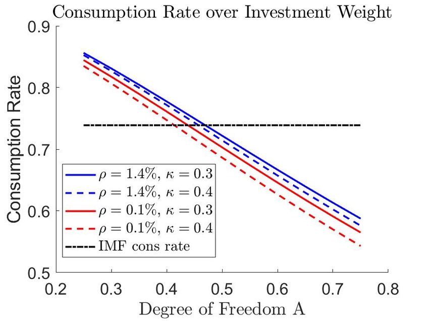
Further characterization and calibration. The optimal consumption rate is
x∗ = 1 − βκ. Society consumes less the higher the discounted shadow value of capital
(x∗t = 1+βϕ1
κ
κ
with ϕk = 1−βκ ), resulting in a consumption rate that decreases in
the capital share of output κ. The other controls depend on the precise form of the
production and energy sectors, but they are not needed to determine the optimal
carbon tax (see Appendix B.1 for further details).
I calibrate the remaining parts of ACE as follows (base calibration). A capital share
of κ = 0.3 and the International Monetary Fund’s (IMF 2020) investment rate forecast
of 1 − x∗ = 26% pin down an annual rate of pure time preference of ρ = 1.4%. Present
world output Y is 10 times (time step) the IMF’s global economic output forecast of
atmospheric carbon dioxide concentration. An extension of ACE can incorporate a declining climate
sensitivity without losing analytic tractability. For ease of exposition, I decided for the simpler climate
system.
14annual
Y2020 = 130 trillion USD (purchasing power parity). The base calibration uses the
carbon cycle of DICE 2013.
4 Policy Results
The SCC is the money-measured present value welfare loss from adding a ton of CO2
to the atmosphere. The Pigovian carbon tax is the SCC along the optimal trajectory
of the economy. In the present model, the SCC is independent of the future path of
the economy. Therefore, this unique SCC is the optimal carbon tax.15
4.1 Base Scenario, Analytics, Decomposition
Appendix B solves for the shadow values and derives the optimal CO2 tax. It is
proportional to output Yt and increases over time at the rate of economic growth as
in Golosov et al. (2014). In contrast to earlier models, ACE avoids summing over
future periods, emission impulse responses, or reservoirs, yielding a simpler and yet
richer description of the dynamic characteristics driving the optimal carbon tax. It
is the first formula pinpointing the tax contribution from carbon versus temperature
dynamics.
Proposition 2 (1) Under the assumptions of section 2, the SCC in (USD-2020-)
money-measured consumption equivalents is
βYtnet U SD
ξ0 (1 − βσ)−1 1,1 σ f orc (1 − βΦ)−1 1,1 = 30
SCCt = (12)
Mpre |{z} | {z } | {z } | {z } tCO2
2.1% 1.1 0.54 4.3
| {z }
U SD
11.5 tCO
2
where [·]1,1 denotes the first element of the inverted matrix in square brackets, and the
numbers rely on the calibration discussed in section 3.
(2) A carbon cycle (equation 6) satisfying mass conservation of carbon implies a factor
(1 − β)−1 in the SCC (equation 12), which is approximately proportional to the inverse
of the rate of pure time preference ρ1 .
The ratio of world output to preindustrial carbon concentrations Mpre sets the units
of the carbon tax. The discount factor β reflects a one-period delay between tem-
15
The present paper calculations the Pigovian tax in the first-best setting, see e.g. Barrage (2019)
for an analysis of how the typical distortions in raising tax revenue modify the Pigovian tax on carbon.
15perature increase and production impact. The damage parameter ξ0 represents the
semi-elasticity of net output with respect to a transformed temperature increase, i.e.,
to an increase of τ1 = exp(ξ1 T1 ). In the absence of climate dynamics, these terms would
imply a carbon tax of 11.50 tCOU SD
2
, or 10 cents per gallon at the pump (2 e-cents per
liter). The interesting thrust making the carbon tax more serious stems from climate
dynamics.
Contribution of carbon dynamics: a major multiplier. Analytic models of
climate change previously captured carbon dynamics in a decay or impulse response
formulation, whereas numeric IAMs incorporate a carbon cycle that models the physical
carbon flows and respects that carbon does not decay. ACE integrates a carbon cycle,
and a Neumann series expansion of βΦ interprets the implications for the carbon tax
P∞
(1 − βΦ)−1 = i=0 β i Φi . (13)
The element [Φi ]1,1 of the transition matrix characterizes how much of the carbon in-
jected into the atmosphere in the present remains in or returns to the atmosphere in pe-
riod i, after cycling through the different carbon reservoirs. E.g., [Φ2 ]1,1 = j Φ1,j Φj,1
P
characterizes the fraction of carbon leaving the atmosphere for layers j ∈ {1, ..., m}
in the first time step and arriving back to the atmosphere in the second time step.
Thus, the term [(1 − βΦ)−1 ]1,1 characterizes in closed form the discounted sum of CO2
persisting in and returning to the atmosphere in all future periods. The discount factor
accounts for the delay between the act of emitting CO2 and the resulting temperature
forcing over the course of time. Quantitatively, the persistence of carbon increases the
U SD
earlier value by a factor of 4.3 and the resulting carbon tax would be almost 50 tCO 2
or
over 40 cents per gallon – ignoring temperature dynamics.
Intuitively, the carbon multiplier [(1 − βΦ)−1 ]1,1 is a form of Keynesian multi-
plier. Our emissions diffuse into different “channels”, but some of these feed back
again into the atmosphere, thereby amplifying the emissions’ effectiveness. Similarly,
[(1 − βΦ)−1 ]1,2 characterizes the long-term forcing contribution from CO2 that is cur-
rently in the shallow ocean. The difference between these multipliers can inform back-
of-the-envelope calculations for the value of different geoengeneering “solutions” to
climate change that channel our CO2 emissions into the ocean or other non-permanent
reservoirs. E.g., channeling emissions into the shallow ocean would relieve the SCC by
[(1I −βΦ)−1 ]1,1 −[(1I −βΦ)−1 ]1,2 U SD
[(1I −βΦ)−1 ]1,1
≈ 67% or 20 tCO2
in absolute terms (ignoring damages from
ocean acidification). This difference in the long-term impact of carbon in the atmo-
16sphere versus the ocean and biosphere also play an important role in evaluating the
impact of uncertainty governing carbon dynamics (Traeger 2021b).
Contribution of temperature dynamics: a net reduction. The terms
[(1 − βσ)−1 ]1,1 σ f orc capture the atmosphere-ocean temperature dynamics resulting
from both delay and persistence. That is, it takes time to warm the atmosphere
and oceans, but once they are warm, they conserve some of this warming. Analogously
to the case of carbon, the expression [(1 − βσ)−1 ]1,1 characterizes the generalized heat
flow that enters, remains, and returns to our atmosphere. Thus, the simple closed-form
expression for the carbon tax in equation (12) captures an infinite double sum: an ad-
ditional ton of carbon emissions today causes radiative forcing in all future periods,
and the resulting radiative forcing in any given period increases the temperature in all
subsequent periods. The parameter σ f orc captures the atmospheric adjustment rate
to radiative forcing absent ocean cooling. Ocean-atmosphere temperature dynamics
reduces the carbon tax by approximately 40%, resulting in the optimal carbon tax of
U SD
30 tCO 2
or 27 cents per gallon (6 e-cents per liter). This carbon tax is somewhat higher
U SD
than Nordhaus’s (2014) optimal carbon tax of 21 tCO 2
for DICE 2013, which has a more
sluggish temperature response and uses a much lower estimate of world output.16
A conceptual implication for policy making. The SCC in equation (12) is
independent of the atmospheric carbon concentration and of the prevailing temperature
level. A corresponding independence of past emissions already prevails in Golosov et al.
(2014), and contradicts the common perception that slacking on climate policy today
will require more mitigation in the future. This result might sound like good news,
but what the model really states is as follows. If we delay policy today, we will not
compensate in our mitigation effort tomorrow, but will live with the consequences
forever. Yet, the result does contain some good news for policy makers and modelers.
Setting the optimal carbon tax requires minimal assumptions about future emission
trajectories and mitigation technologies. The policy-maker sets an optimal price of
carbon, and the economy determines the resulting optimal emission trajectory. The
common intuition that the SCC ought to increase in the CO2 concentration and the
16
Golosov et al. (2014) and Gerlagh & Liski (2018b) use an emission response model similar to the
common carbon cycle models that I adopt here. Their models do not explicitly incorporate radiative
forcing, temperature dynamics, and damages as a function of temperature. However, Gerlagh &
Liski (2018b) introduce a delay between peak emissions and peak damages, motivated by the missing
temperature component. This delay multiplier contributes a factor of .45 in their closest scenario
(“Nordhaus”), which cuts the tax a little more than ACE’s factor of 1.4 · 0.42 ≈ .6, derived from an
explicit model of temperature dynamics calibrated to MAGICC6.0.
17prevailing temperature level results from the convexity of damages in temperature. Yet,
what common intuition overlooks is that CO2 traps (absorbs) energy only in a certain
range of wavelengths that is increasingly saturated. As a result, warming is logarithmic
in the prevailing atmospheric CO2 concentration (equation 7), and the marginal ton’s
warming impact is proportional to the inverse of the prevailing concentration.
4.2 Discounting and Time Preference
It is well known that the consumption discount rate plays a crucial role in valuing long-
run impacts (Nordhaus 2007, Weitzman 2007). Finding (2) in Proposition 2 is different.
It states that the interaction of pure time preference and carbon cycle dynamics is the
main sensitivity when it comes to discounting. The proposition ties this sensitivity
directly to the fact that carbon does not decay, but only cycles through the different
reservoirs; a fraction of our current emissions remains in or returns to the atmosphere in
the long run. In DICE 2013’s carbon cycle, about 6% stay in the atmosphere forever.17
The growth contribution to discounting is less relevant because the damages from
climate change grow approximately proportionally to consumption, which offsets the
growth-induced reduction in future marginal value. The contribution of temperature
dynamics is less sensitive to time preference because heat is not conserved.18 The
extreme sensitivity weakens as we depart from log utility as van den Bijgaart et al.
(2016) and Rezai & van der Ploeg (2016) elaborate with approximate formulas and
numeric simulations. As we start reducing the elasticity of intertemporal substitution,
we clean up more of our historic sins along the optimal trajectory, and worry a little
less about their long-run consequences.
The high sensitivity to pure time preference, coupled with a low sensitivity to the
consumption discount rate, has an interesting policy implication. The US Circular
A-4 by the Office of Management and Budget prescribes a consumption discount rate
of 3%.19 It does not give any direct guidance regarding its composition, leaving a degree
17
The maximal eigenvalue of the carbon cycle’s transition matrix Φ is unity and the corresponding
eigenvector governs the long-run distribution (as the transitions corresponding to all other eigenvectors
are damped). The first entry of the corresponding eigenvector is 0.06.
18
Heat is constantly exchanged with outer space. Golosov et al.’s (2014) SCC formula already shows
a related sensitivity to pure time preference, arising from modeling emissions as a convex combination
of decaying and non-decaying carbon. In their published revision, Gerlagh & Liski (2018b) explain how
the non-decaying carbon box results from a carbon cycle. Finding (2), which was first published in
the working paper version of the present paper (Traeger 2015), is related in spirit, but directly factors
out the sensitivity factor (1 − β)−1 resulting from mass conservation in the carbon cycle formulation.
19
More precisely, cost-benefit analysis is undertaken with both a 3% and a 7% discount rate where
18of freedom to the modelers of the Interagency Working Group on the US’ federal SCC
that I show to have a huge impact on the SCC’s magnitude. For this purpose, first,
note that the SCC formula holds independently of the economy’s growth rate. Second,
section 5.2 develops a more sophisticated investment model showing that ACE can
easily match observed consumption-investment rates with any of the present choices of
time preference.
The base calibration in Section 3.3 implies a rate of pure time preference of ρ =
1.4%. Instead, Drupp et al.’s (2018) recent expert survey suggests ρ = 0.5% as the
median response, changing the SCC and its components to
βYtnet U SD
ξ0 (1 − βσ)−1 1,1 σ f orc (1 − βΦ)−1 1,1 =
SCCt = 30
HH 72
.
Mpre |{z} | {z } | {z } | {z } tCO2
2.1% 1.1
1.3 0.54 4.3
8.4
| {z }
12.5 U SD
11.5
tCO2
The formula emphasizes that, under certainty, the main determinant of the optimal
carbon tax is the interaction of time preference and carbon dynamics, doubling its
U SD
contribution to a factor of 8. Overall, the SCC increases almost 2.5 times to 72 tCO 2
or
63 cents per gallon at the pump (≈ 14 e-cents per liter).
More sophisticated calibrations of time preference than in the present paper, using
the long-run-risk model of asset pricing, deliver even lower rates while matching risk-
free rate and risk premia substantially better, e.g., Bansal et al. (2012) calibrate a
rate of ρ = 0.11%.20 The Stern (2007) Review argues for the rate of ρ = 0.1% for
normative reasons. Similarly, low rates of pure time preference can arise if observed
market equilibria are interpreted as reflecting individual life-cycle choices in the absence
of bequest motives (Schneider et al. 2013) and when distinguishing consumption choice
from political long-term decision making and voting (Hepburn 2006). A rate of pure
the 3% reflects consumption discounting, and the 7% pre-tax capital interest. In addition, a third
rate between 1-3% can be suggested if future generations are affected. The 3% rate was employed as
the base rate under the Obama administration and is likely to return with the Biden administration.
For the 3% rate, the Interagency Report on the SCC found a 2020 SCC estimate of 26 2007-U SD
tCO2 using
2007-U SD
a cross section of models. They also report SCCs of 7 and 42 tCO2 for consumption discount rates
of 5 and 2.5%, respectively.
20
Traeger (2012a) shows how uncertainty-based discounting by an agent whose risk aversion does not
coincide with her consumption-smoothing preference (falsely) manifests itself as pure time preference
in the standard economic model.
19time preference of ρ = 0.1% changes the SCC and its components as follows
βYtnet U SD
ξ0 (1 − βσ)−1 1,1 σ f orc (1 − βΦ)−1 1,1 =
SCCt = 30
HH 276
.
Mpre |{z} | {z } | {z } | {z } tCO2
2.1% 1.1
1.5 0.54 4.3
26
| {z }
13 U SD
11.5
tCO2
This ninefold increase of the SCC is, once more, mostly driven by the interaction of time
preference with the carbon cycle. Temperature dynamics now only reduces the SCC
by 20% as also the (moderate) temperature persistence obtains more weight relative
to the short-term warming delay. The present evaluations use equation (12) without
further recalibration. As a result, these evaluations would correspond to investment
rates of 28.5% and 30% rather than the observation-based 26% used in the original
model calibration. From a normative point of view, such a difference is warranted (but
would suggest that policy should also increase other investments). In response to the
Stern (2007) Review, which applies log-utility in combination with ρ = 0.1%, Nord-
haus (2007,2014) rejects the resulting high values of the SCC based on this descriptive
inconsistency. Yet, the long-run risk model calibrates such a low time preference and
explains observed investments and risk premia far better than any IAM. It would ex-
plain the high investment rates noted above as a result of the missing investment risks
in these IAMs. More generally, Section 5.2 distinguishes consumption and investment
sectors, casting into doubt the somewhat simplistic calibration of pure time preferences
common to many IAMs. The resulting modification easily reconciles low rates of pure
time preference with observed investment rates, also under certainty. The approach
results in a slight modification of equation (12), which further increases the SCC to
U SD U SD
the values shown in Table 1, 75 tCO 2
and 290 tCO2
, respectively.
4.3 DICE’s Carbon Cycle versus Impulse Response
DICE’s climate dynamics has recently been criticized for scientific inaccuracy (Mattauch
et al. 2020, Van der Ploeg et al. 2020). ACE’s base scenario already avoids the main
target of the criticism, DICE’s overly sluggish temperature response. But also the car-
bon cycle responds a little more sluggishly when compared to scientific models (Van
der Ploeg et al. 2020). Joos et al. (2013) provides a simple emulation of scientific
carbon cycle models. Instead of tracking carbon through different (at times complex)
reservoirs, the authors calibrate the atmospheric impulse response for a variety of car-
bon cycle models, including the best fit to a state of the art ensemble (CMIP 5). The
20approach distributes a ton of carbon emitted into 4 different “boxes”. These boxes
no longer correspond to physical reservoirs; instead these boxes are characterized by
unique atmospheric life-times. The amount of atmospheric carbon in period t resulting
from a unit of today’s (t=0) emissions is
3
X t
∆M1,t = a0 + ai exp − ,
i=1
τi
where a = (a0 , a1 , a2 , a3 )> characterizes the fraction of carbon going into a particular
box. The fraction a0 stays in the atmosphere forever and the fractions ai of today’s
emission unit has an e-folding time τi .21 The IPCC (2013) uses this quantitative model
to calculate global warming potentials.
This box model is formally equivalent to the usual carbon cycle model with the
following modifications. First, carbon is released not only into the atmosphere, but into
all boxes. In addition, some of the carbon simply vanishes immediately ( 3i=0 a0 < 1).
P
Formally, the weight vector a replaces the unit vector e1 channeling emissions (only)
into the atmosphere in equation (6). As a result, the SCC will become the ai -weighted
sum of the different boxes’ shadow values. Second, all boxes correspond to atmospheric
carbon and, thus, contribute to radiative forcing changing equation (7) to
P3
Mi,t +Gt
log i=0
Mpre
Ft = η . (14)
log 2
Third, the transition matrix is diagonal as carbon no longer moves across boxes.
As a result, the inversion of the matrix in the SCC formula becomes trivial and
[(1 − βΦ)−1 ]i,i = 1−γ1 i β , where the coefficients γi = exp − step
τi
are the (diagonal)
entries of the transition matrix; the first diagonal entry corresponds to τ0 = ∞ and
γ0 = 1, and step = 10 represents the time step. I emphasize that all boxes reflect at-
mospheric carbon and no longer have a direct physical counterpart; they approximate
the different response times of various carbon sinks.
The resulting SCC formula becomes (see Appendix B.3)
3
!
net
βYt a0 X ai
(1 − βσ)−1 1,1 σ f orc
SCCt = + (15)
Mpre 1−β i=1
1 − γi β
21
The e-folding time represents the time at which only a fraction corresponding to one over the
Euler’s number remains in the atmosphere. The corresponding e-folding times (half-lifes) are τ1 =
394.4 (273), τ2 = 36.54 (25), and τ3 = 4.304 (3) years. Note the notational difference between
e-folding time τ (only used in the present subsection) and generalized temperature τ .
21You can also read