WETCHIMP-WSL: intercomparison of wetland methane emissions models over West Siberia
←
→
Page content transcription
If your browser does not render page correctly, please read the page content below
Biogeosciences, 12, 3321–3349, 2015
www.biogeosciences.net/12/3321/2015/
doi:10.5194/bg-12-3321-2015
© Author(s) 2015. CC Attribution 3.0 License.

WETCHIMP-WSL: intercomparison of wetland methane
emissions models over West Siberia
T. J. Bohn1 , J. R. Melton2 , A. Ito3 , T. Kleinen4 , R. Spahni5,6 , B. D. Stocker5,7 , B. Zhang8 , X. Zhu9,10,11 ,
R. Schroeder12,13 , M. V. Glagolev14,15,16,17 , S. Maksyutov3,16 , V. Brovkin4 , G. Chen18 , S. N. Denisov19 ,
A. V. Eliseev19,20 , A. Gallego-Sala21 , K. C. McDonald12 , M.A. Rawlins22 , W. J. Riley11 , Z. M. Subin11 , H. Tian8 ,
Q. Zhuang9 , and J. O. Kaplan23
1 School  of Earth and Space Exploration, Arizona State University, Tempe, AZ, USA
2 Canadian   Centre for Climate Modelling and Analysis, Environment Canada, Victoria, BC, Canada
3 National Institute for Environmental Studies, Tsukuba, Japan
4 Max Planck Institute for Meteorology, Hamburg, Germany
5 Climate and Environmental Physics, Physics Institute, University of Bern, Bern, Switzerland
6 Oeschger Centre for Climate Change Research, University of Bern, Bern, Switzerland
7 Department of Life Sciences, Imperial College, Silwood Park Campus, Ascot, UK
8 International Center for Climate and Global Change Research and School of Forestry and Wildlife Sciences, Auburn

University, Auburn, AL, USA
9 Department of Earth, Atmospheric, and Planetary Sciences, Purdue University, West Lafayette, IN, USA
10 Natural Resource Ecology Laboratory, Colorado State University, Fort Collins, CO, USA
11 Earth Sciences Division, Lawrence Berkeley National Laboratory, Berkeley, CA, USA
12 City College of New York, City University of New York, New York, NY, USA
13 Institute of Botany, University of Hohenheim, Stuttgart, Germany
14 Moscow State University, Moscow, Russia
15 Institute of Forest Science, Russian Academy of Sciences, Uspenskoe, Russia
16 Laboratory of Computational Geophysics, Tomsk State University, Tomsk, Russia
17 Yugra State University, Khanty-Mantsiysk, Russia
18 Oak Ridge National Laboratory, Oak Ridge, TN, USA
19 A. M. Obukhov Institute of Atmospheric Physics, Russian Academy of Sciences, Moscow, Russia
20 Kazan Federal University, Kazan, Russia
21 Department of Geography, University of Exeter, Exeter, UK
22 Department of Geosciences, University of Massachusetts, Amherst, MA, USA
23 Institute of Earth Surface Dynamics, University of Lausanne, Lausanne, Switzerland

Correspondence to: T. J. Bohn (theodore.bohn@asu.edu)

Received: 10 December 2014 – Published in Biogeosciences Discuss.: 30 January 2015
Revised: 29 April 2015 – Accepted: 30 April 2015 – Published: 3 June 2015

Abstract. Wetlands are the world’s largest natural source        could potentially liberate large amounts of labile carbon
of methane, a powerful greenhouse gas. The strong sensi-         over the next 100 years. However, global models disagree
tivity of methane emissions to environmental factors such        as to the magnitude and spatial distribution of emissions,
as soil temperature and moisture has led to concerns about       due to uncertainties in wetland area and emissions per unit
potential positive feedbacks to climate change. This risk is     area and a scarcity of in situ observations. Recent intensive
particularly relevant at high latitudes, which have experi-      field campaigns across the West Siberian Lowland (WSL)
enced pronounced warming and where thawing permafrost            make this an ideal region over which to assess the per-

Published by Copernicus Publications on behalf of the European Geosciences Union.
3322                                                T. J. Bohn et al.: Intercomparison of wetland methane emissions models

formance of large-scale process-based wetland models in a             Process-based models are crucial for increasing our un-
high-latitude environment. Here we present the results of          derstanding of the response of wetland CH4 emissions to cli-
a follow-up to the Wetland and Wetland CH4 Intercom-               mate change. Large-scale biogeochemical models, especially
parison of Models Project (WETCHIMP), focused on the               those embedded within earth system models, are particularly
West Siberian Lowland (WETCHIMP-WSL). We assessed                  important for estimating the magnitudes of feedbacks to cli-
21 models and 5 inversions over this domain in terms of            mate change (e.g., Gedney et al., 2004; Eliseev et al., 2008;
total CH4 emissions, simulated wetland areas, and CH4              Koven et al., 2011). However, as shown in the global Wet-
fluxes per unit wetland area and compared these results            land and Wetland CH4 Intercomparison of Models Project
to an intensive in situ CH4 flux data set, several wetland         (WETCHIMP; Melton et al., 2013; Wania et al., 2013), there
maps, and two satellite surface water products. We found           was wide disagreement among large-scale models as to the
that (a) despite the large scatter of individual estimates,        magnitude of global and regional wetland CH4 emissions,
12-year mean estimates of annual total emissions over the          in terms of both wetland areas and CH4 emissions per unit
WSL from forward models (5.34 ± 0.54 Tg CH4 yr−1 ), in-            wetland area. These discrepancies were due in part to the
versions (6.06 ± 1.22 Tg CH4 yr−1 ), and in situ observations      large variety of schemes used for representing hydrologi-
(3.91 ± 1.29 Tg CH4 yr−1 ) largely agreed; (b) forward mod-        cal and biogeochemical processes, in part to uncertainties in
els using surface water products alone to estimate wetland         model parameterizations, and in part to the sparseness of in
areas suffered from severe biases in CH4 emissions; (c) the        situ observations with which to evaluate model performance
interannual time series of models that lacked either soil ther-    (Melton et al., 2013).
mal physics appropriate to the high latitudes or realistic emis-      In addition to these challenges on the global scale, the
sions from unsaturated peatlands tended to be dominated by         unique characteristics of high-latitude environments pose
a single environmental driver (inundation or air temperature),     further problems for biogeochemical models. For example,
unlike those of inversions and more sophisticated forward          much of the northern land surface is underlain by permafrost,
models; (d) differences in biogeochemical schemes across           which impedes drainage (Smith et al., 2005) and stores an-
models had relatively smaller influence over performance;          cient carbon (Koven et al., 2011) via temperature-dependent
and (e) multiyear or multidecade observational records are         constraints on carbon cycling (Schuur et al., 2008). Similarly,
crucial for evaluating models’ responses to long-term climate      peat soils and winter snowpack can thermally insulate soils
change.                                                            (Zhang, 2005; Lawrence and Slater, 2008, 2010), dampening
                                                                   their sensitivities to interannual variability in climate. Several
                                                                   commonly used global biogeochemical models (e.g., Tian et
                                                                   al., 2010; Hopcroft et al., 2011; Hodson et al., 2011; Kleinen
                                                                   et al., 2012) lack representations of some or all of these pro-
1   Introduction                                                   cesses.
                                                                      The prevalence of peatlands in the high-latitudes poses
Methane (CH4 ) emissions from high-latitude wetlands are an        further challenges to modeling (Frolking et al., 2009). Peat-
important component of the global climate system. CH4 is           lands are a type of wetland containing deep deposits of highly
an important greenhouse gas, with approximately 34 times           porous, organic-rich soil, formed over thousands of years
the global warming potential of carbon dioxide (CO2 ) over a       under waterlogged and anoxic conditions, which inhibit de-
century time horizon (IPCC, 2013). Globally, wetlands are          composition (Gorham, 1991; Frolking et al., 2011). Within
the largest natural source of CH4 emissions to the atmo-           the porous soil, the water table is often only a few centime-
sphere (IPCC, 2013). Because wetland CH4 emissions are             ters below the surface, leading to anoxic conditions and CH4
highly sensitive to soil temperature and moisture conditions       emissions even when no surface water is present (Saarnio
(Saarnio et al., 1997; Friborg et al., 2003; Christensen et al.,   et al., 1997; Friborg et al., 2003; Glagolev et al., 2011).
2003; Moore et al., 2011; Glagolev et al., 2011; Sabrekov          This condition can lead to an underestimation of wetland
et al., 2014), there is concern that they will provide posi-       area when using satellite surface water products as inputs
tive feedback to future climate warming (Gedney et al., 2004;      to wetland methane emissions models. In addition, trees and
Eliseev et al., 2008; Ringeval et al., 2011). This risk is par-    shrubs are found with varying frequency in peatlands (e.g.,
ticularly important in the world’s high latitudes because they     Shimoyama et al., 2003; Efremova et al., 2014), interfering
contain nearly half of the world’s wetlands (Lehner and Döll,      with the detection of inundation. Furthermore, the water table
2004) and because the high latitudes have been and are fore-       depth within a peatland is typically heterogeneous, varying
cast to continue experiencing more rapid warming than else-        on the scale of tens of centimeters as a function of microto-
where (Serreze et al., 2000; IPCC, 2013). Adding to these          pography (hummocks, hollows, ridges, and pools; Eppinga
concerns is the potential liberation (and possible conversion      et al., 2008). Models vary widely in their representations of
to CH4 ) of previously frozen, labile soil carbon from thawing     wetland soil moisture conditions, ranging from schemes that
permafrost over the next century (Christensen et al., 2004;        do not explicitly consider the water table position (e.g., Hod-
Schuur et al., 2008; Koven et al., 2011; Schaefer et al., 2011).   son et al., 2011) to a single uniform water table depth for

Biogeosciences, 12, 3321–3349, 2015                                                     www.biogeosciences.net/12/3321/2015/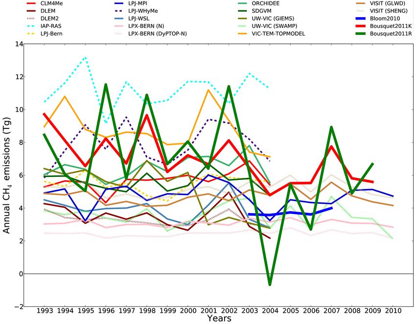
T. J. Bohn et al.: Intercomparison of wetland methane emissions models                                                           3323

Figure 1. Map of the West Siberian Lowland (WSL). (a) Limits of domain (brown) and peatland distribution (cyan), taken from Sheng et
al. (2004); lakes of area > 1 km2 (blue) taken from Lehner and Döll (2004); permafrost zone boundaries after Kremenetski et al. (2003);
CH4 sampling sites from Glagolev et al. (2011), denoted by red circles. (b) Dominant land cover at 25 km derived from MODIS-MOD12Q1
500 m land cover classification (Friedl et al., 2010).

each grid cell (e.g., Zhuang et al., 2004) to more sophisti-          land inventories (Sheng et al., 2004; Peregon et al., 2008,
cated schemes that allow for sub-grid heterogeneity in the            2009).
water table (e.g., Bohn et al., 2007, 2013; Ringeval et al.,             Our primary goal in this study is to determine how well
2010; Riley et al., 2011; Kleinen et al., 2012; Stocker et al.,       current global large-scale models capture the dynamics of
2014; Subin et al., 2014). Finally, peatland soils can be highly      high-latitude wetland CH4 emissions. To this end, we assess
acidic and nutrient-poor, and much of the available carbon            the performance of 21 large-scale wetland CH4 emissions
substrate can be recalcitrant (Clymo et al., 1984; Dorrepaal          models over West Siberia, relative to in situ and remotely
et al., 2009). While some models attempt to account for the           sensed observations as well as inverse models. We examine
effects of soil chemical conditions such as pH, redox poten-          both spatial and temporal accuracy, including seasonal and
tial, and nutrient limitation (e.g., Zhuang et al., 2004; Riley       interannual variability, and estimate the relative influences of
et al., 2011; Sabrekov et al., 2013; Spahni et al., 2013), not        environmental drivers on model behaviors. We identify the
all do.                                                               dominant sources of error and the model features that may
   Given the potential problems of parameter uncertainty and          have caused them. Finally, we make recommendations as to
equifinality (Tang and Zhuang, 2008; van Huissteden et al.,           which model features are necessary for accurate simulations
2009) and computational limitations when wetland compo-               of high-latitude wetland CH4 emissions and which types of
nents are embedded within global climate models, it is im-            observations would help improve future efforts to constrain
portant to determine which model features are necessary               model behaviors.
to simulate high-latitude peatlands accurately and to con-
strain parameter values with observations. Until recently,
the evaluation of large-scale wetland CH4 emissions mod-              2     Methods
els has been difficult, due to the sparseness of in situ and
atmospheric CH4 observations. However, observations from              2.1    Spatial domain
the West Siberian Lowland (WSL) now offer the opportu-
nity to assess model performance, thanks to recent inten-             The West Siberian Lowland (WSL) occupies approximately
sive field campaigns (Glagolev et al., 2011), aircraft profiles       2.5 million km2 in northern central Eurasia, spanning from
(Umezawa et al., 2012), tall-tower observations (Sasakawa et          50 to 75◦ N and 60 to 95◦ E (Fig. 1a). This region is bounded
al., 2010; Winderlich et al., 2010), and high-resolution wet-         on the west by the Ural Mountains; on the east by the Yeni-
                                                                      sei River and the Central Siberian Plateau; on the north by the

www.biogeosciences.net/12/3321/2015/                                                          Biogeosciences, 12, 3321–3349, 2015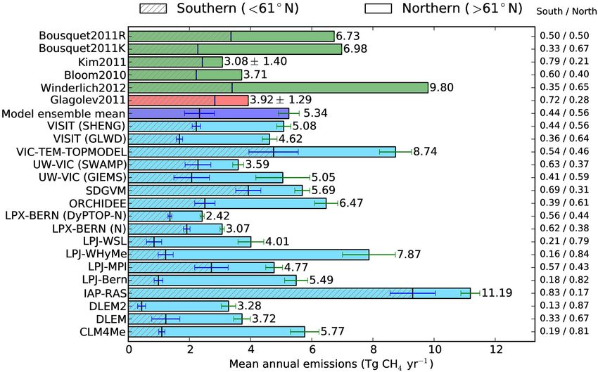
3324                                                T. J. Bohn et al.: Intercomparison of wetland methane emissions models

Arctic Ocean; and on the south by the Altai Mountains and          we will exclude them from our definition. Unfortunately, ex-
the grasslands of the Eurasian Steppe (Sheng et al., 2004).        plicit observations of lake depths are lacking for all but the
The WSL contains most of the drainage areas of the Ob’ and         deepest lakes; therefore, we will instead use an area threshold
Irtysh rivers, as well as the western tributaries of the Yenisei   (1 km2 ) to identify permanent lakes. This definition of wet-
River, all of which drain into the Arctic Ocean. Permafrost in     lands therefore includes all peatlands (inundated or not), sea-
various forms (continuous, discontinuous, isolated, and spo-       sonally inundated non-peatland soils (e.g., river floodplains),
radic) covers more than half of the area of the WSL, from          and small ponds or lakes but excludes rivers and large lakes.
the Arctic Ocean south to approximately 60◦ N, with con-              We define “surface water” as all freshwater above the soil
tinuous permafrost occurring north of 67◦ N (Kremenetski et        surface, i.e., the superset of inundation, lakes, and rivers.
al., 2003). The region’s major biomes (Fig. 1b) consist of the     We define “inundation” as temporary (present for less than
treeless tundra north of 66◦ N, approximately coincident with      1 year) standing water above the soil surface; “lakes” as per-
continuous permafrost; the taiga forest belt between 55 and        manent water bodies (present for more than 1 year) exceed-
66◦ N; and the grasslands of the steppe south of 55◦ N.            ing 1 km2 in area; and “rivers” as channels that carry turbu-
   Wetlands occupy 600 000 km2 , or about 25 % of the land         lent water. Surface water therefore includes areas that do not
area of the WSL, primarily in the taiga and tundra zones           emit large amounts of CH4 , such as rivers, and also excludes
(Sheng et al., 2004). The vast majority of these wetlands          some CH4 -emitting areas such as non-inundated peatlands.
are peatlands, which have peat depths ranging from 50 cm              For models, we will use the term “CH4 -producing area”
to over 5 m and which comprise a total soil carbon pool of         to refer to the area over which CH4 production is simulated,
70 Pg C (Sheng et al., 2004). Numerous field studies have          which might not coincide exactly with the areas of actual or
documented strong methane emissions from these peatlands,          simulated wetlands.
particularly those south of the southern limit of permafrost
(e.g., Sabrekov et al., 2014; Sasakawa et al., 2012; Glagolev      2.3   Observations and inversions
et al., 2011, 2012; Friborg et al., 2003; Shimoyama et al.,
2003; Panikov and Dedysh, 2000). Permanent water bodies,           Table 1 lists the various observations and inversions that
ranging in size from lakes 100 km2 in area to pools only a         we used in this study. We considered four wetland map
few meters across, are comingled with wetlands throughout          products over the WSL, all of which have been used in
the domain (Lehner and Döll, 2004; Repo et al., 2007; Ep-          high-latitude wetland carbon studies. Two of them are re-
pinga et al., 2008). Notable concentrations of lakes are found     gional maps specific to the WSL: Sheng et al. (2004), de-
(a) north of the Ob’ River between 61 and 64◦ N and 68 and         noted by “Sheng2004”, and Peregon et al. (2008), denoted by
80◦ E; (b) west of the confluence of the Ob’ and Irtysh rivers     “Peregon2008”. Both Sheng 2004 and Peregon2008 used the
between 59 and 61◦ N and 64 and 70◦ E; and (c) on the Yamal        1 : 2500 000-scale map of Romanova (1977): Peregon2008
Peninsula north of 68◦ N.                                          was entirely based on the Romanova map, while Sheng2004
   Because the vegetative and soil conditions vary substan-        used the Romanova map north of 65◦ N and used the 1 :
tially across the domain, we have divided it into two halves       100 000-scale maps of Markov (1971) and Matukhin and
of approximately equal size along 61◦ N latitude. The region       Danilov (2000) elsewhere. Both of these maps delineate the
north of this line contains permafrost, while the region south     extents of peatlands, including ponds and lakes smaller than
of the line is essentially permafrost-free.                        1 km2 in area. The Sheng2004 product additionally includes
                                                                   a separate layer delineating lakes larger than 1 km2 . The
2.2    Terminology                                                 Peregon2008 product distinguishes between various wetland
                                                                   subtypes (e.g., sphagnum- or sedge-dominated bogs and high
Estimating wetland CH4 emissions over large scales requires        palsa mires). The third map is the Northern Circumpolar Soil
accurately delineating the wetland area over which CH4             Carbon Database (NCSCD; Tarnocai et al., 2009), an inven-
emissions can occur. Unfortunately, “wetland” definitions          tory of carbon-rich soils, including peatlands, within the Arc-
vary within the scientific community (Mitsch and Gosselink,        tic permafrost region. Models that have used this database
2000). For the purposes of estimating CH4 emissions, the           have taken the Histel and Histosol delineations to be synony-
key characteristics include anoxia and available labile carbon     mous with peatlands. The fourth map is the wetland layer
substrate; therefore, we will adopt the definition proposed by     (GLWD-3, excluding the rivers and lakes of area > 1 km2 of
Canada’s National Wetlands Working Group (Tarnocai et al.,         layers GLWD-1 and GLWD-2) of the Global Lakes and Wet-
1988): land that is saturated with water for long enough to        land Database (GLWD; Lehner and Döll, 2004), in which
promote wetland or aquatic processes as indicated by poorly        wetland extents are the union of polygons from four differ-
drained soils, hydrophytic vegetation, and various kinds of        ent global databases.
biological activity which are adapted to a wet environment.           Two global time-varying surface water products derived
Because permanent, deep (> 2m) open-water bodies are sub-          from remote-sensing observations were also examined in this
ject to additional processes (e.g., allocthonous carbon inputs,    study: the Global Inundation Extent from Multi-Satellites
wind-driven mixing of the water column; Pace et al., 2004),        (GIEMS; Prigent et al., 2007; Papa et al., 2010), derived

Biogeosciences, 12, 3321–3349, 2015                                                    www.biogeosciences.net/12/3321/2015/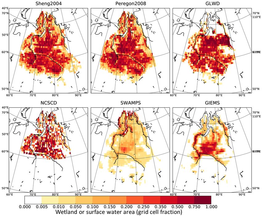
Table 1. Observations and inversions used in this study.
Name Reference Description Temporal Temporal Spatial domain Spatial resolution
domain resolution
Wetland maps
Sheng2004 Sheng et al. (2004) Wetland map of WSL based on digitization of regional maps Second half of Static map Western Siberia 1 : 2 500 000 north of
of Markov (1971), Matukhin and Danilov (2000), and Ro- 20th century 65◦ N, 1 : 1 000 000
manova et al. (1977). Supplemented with peat cores. south of 65◦ N
Peregon2008 Peregon et al. (2008) Wetland map of WSL based on digitization of regional map of Second half of Static map Western Siberia 1 : 2 500 000
Romanova et al. (1977). Wetland types identified by remote 20th century
sensing and field validation.
Northern Circumpolar Tarnocai et al. (2009) Map of wetlands across the northern circumpolar permafrost Second half of Static map Northern 1 : 2 500 000
Soil Carbon Database region. Over the WSL, based on maps of Fridland (1988) and 20th century circumpolar
(NCSCD) Naumov (1993). permafrost
region
www.biogeosciences.net/12/3321/2015/
Global Lake and Wetland Lehner and Döll (2004) Global lake and wetland map. Wetlands were the union of Second half of Static map Global 1 : 1 000 000
Database (GLWD) four global data sets. 20th century
Surface Water
Global Inundation Extent Papa et al. (2010) Remote-sensing inundation product based on visible 1993–2004 Daily, Global 25 km equal-area grid, ag-
from Multi-Satellites (AVHRR) and active (SSM/I) and passive (ERS) microwave aggregated gregated
(GIEMS) sensors. to monthly to 0.5◦ × 0.5◦
Surface Water Schroeder et al. (2010) Remote-sensing inundation product based on active 1992–2013 Daily, Global 25 km equal-area grid, ag-
Microwave Product (SeaWinds-on-QuikSCAT, ERS, and ASCAT) and pas- aggregated gregated
Series (SWAMPS) sive (SSM/I, SSMI/S) microwave sensors. to monthly to 0.5◦ × 0.5◦
CH4 Inventory
Glagolev2011 Glagolev et al. (2011) In situ flux sampling along transect spanning West Siberia, 2006–2010 Monthly Western Siberia 0.5◦ × 0.5◦
2006–2010; statistical model of fluxes as function of wetland climatology
T. J. Bohn et al.: Intercomparison of wetland methane emissions models
type applied to map of Peregon et al. (2008).
CH4 Inversions
Bloom2010 Bloom et al. (2010) Global optimization of relationship between SCIAMACHY 2003–2007 Annual Global 3◦ × 3◦
atmospheric CH4 concentrations (Bovensmann et al., 1999),
NCEP/NCAR surface temperatures (Kalnay et al., 1996), and
GRACE gravity anomalies (Tapley et al., 2004).
Bousquet2011R Bousquet et al. (2011), Global inversion using LMDZ with Matthews and Fung 1993–2009 Monthly Global 1◦ × 1◦ resolution for prior,
Bousquet et al. (2006) (1987) inventory as the wetland prior. multiplied by single coeffi-
cient for all of boreal Asia
Bousquet2011K Bousquet et al. (2011), Global inversion using LMDZ with emissions from Kaplan 1993–2009 Monthly Global 1◦ × 1◦ resolution for prior,
Bousquet et al. (2006) (2002) as the wetland prior. multiplied by single coeffi-
cient for all of boreal Asia
Kim2011 Kim et al. (2011) Global inversion, with Glagolev et al. (2010) as prior in WSL 2002–2007 Monthly Regional 1◦ × 1◦ resolution for prior,
and with Fung et al. (1991) elsewhere. climatology multiplied by single coeffi-
cient for all of WSL
Winderlich2012 Winderlich (2012), Regional inversion over West Siberia, with Kaplan (2002) as 2009 Monthly Regional 1◦ × 1◦ resolution for both
Schuldt et al. (2013) the wetland prior. climatology prior and coefficients over
WSL
Biogeosciences, 12, 3321–3349, 2015
3325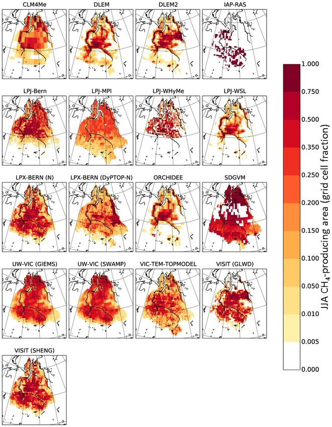
3326                                                T. J. Bohn et al.: Intercomparison of wetland methane emissions models

from visible and near-infrared (AVHRR) and active (SSM/I)          al. (2011) used the Laboratoire de Météorologie Dynamique
and passive (ERS) microwave sensors over the period 1993–          general circulation model (LMDZ; Hauglustaine et al., 2004)
2004, and the Surface Water Microwave Product Series               atmospheric transport model on a 3.75◦ × 2.5◦ grid to esti-
(SWAMPS; Schroeder et al., 2010), derived from active              mate monthly CH4 emissions at a 1◦ × 1◦ resolution for the
(SeaWinds-on-QuikSCAT, ERS, and ASCAT) and passive                 period 1993–2009, optimizing atmospheric concentrations of
(SSM/I, SSMI/S, AMSR-E) microwave sensors over the pe-             several gases, including CH4 , relative to global surface ob-
riod 1992–2013. For both products, surface water area frac-        servation networks, for both inversions. The Matthews and
tions (Fw ) were aggregated from their native 25 km equal-         Fung (1987) emissions inventory was the prior for wetland
area grids to a 0.5◦ × 0.5◦ geographic grid and from daily         emissions in the Bousquet2011R inversion, while the Ka-
to monthly temporal resolution, for consistency with model         plan (2002) emissions were the prior for the Bousquet2011K
results.                                                           inversion. In both cases, a single, spatially uniform set of
   For CH4 emissions, our primary reference for in situ obser-     monthly coefficients was derived for each of 11 large re-
vations was the estimate of Glagolev et al. (2011), which we       gions of the globe. The region containing the WSL was bo-
will refer to as “Glagolev2011”. The Glagolev2011 product          real Asia (in which the WSL makes up the majority of the
consists of both a database of over 2000 individual cham-          wetlands). Consequently, spatial patterns in estimated emis-
ber observations from representative landforms at each of          sions at the scale of 1◦ × 1◦ were identical to those of the
36 major sites over the period 2006–2010 (Fig. 1a) and a           prior emissions; only the regional total emissions were con-
map of long-term average emissions created by applying the         strained by the inversions. The 17-year record length of the
mean observed emissions to the wetlands of the Peregon2008         Bousquet2011 inversions made them appealing candidates
map as a function of wetland type. It is worth noting that         for investigating the sensitivities of emissions to interannual
the Glagolev2011 product is currently undergoing a revision        variability in environmental drivers. Bloom et al. (2010) did
based on higher-resolution maps, which will lead to a sub-         not use an atmospheric transport model, but rather optimized
stantial increase in annual emissions from the taiga zone,         the parameters in a simple model relating observed atmo-
due to a larger spatial extent of high-emitting wetland types      spheric CH4 concentrations from the Scanning Imaging Ab-
(Glagolev et al., 2013). Possible changes to emissions in the      sorption Spectrometer for Atmospheric Chemistry (SCIA-
tundra zone (in the northern half of the WSL) are not yet          MACHY; Bovensmann et al., 1999) on the Envisat satellite to
known. We consider this product’s large uncertainty in our         observed surface temperatures from the National Center for
evaluation of model predictions.                                   Environmental Prediction/National Center for Atmospheric
   We also considered emissions estimates from five inver-         Research (NCEP/NCAR) weather analyses (Kalnay et al.,
sions. Two of them were regional: “Kim2011” (Kim et al.,           1996) and gravity anomalies from the Gravity Recovery and
2011) and “Winderlich2012” (Winderlich, 2012; Schuldt et           Climate Experiment satellite (GRACE; Tapley et al., 2004),
al., 2013). Kim et al. (2011) used an earlier version of           under the assumption that gravity anomalies are indicative
Glagolev2011 (Glagolev et al., 2010) at a 1◦ × 1◦ resolu-          of large-scale surface and near-surface water anomalies. The
tion as their prior distribution for wetland emissions within      Bloom2010 inversion covered the period 2003–2007, at a
the atmospheric transport model NIES-TM (Maksyutov et              3◦ × 3◦ resolution.
al., 2008) over the period 2002–2007. Kim et al. (2011)
derived 12 climatological average monthly (spatially uni-          2.4   Models
form) coefficients for wetland emissions to optimize atmo-
spheric CH4 concentrations over the WSL relative to ob-            Among the participating models (Table 2) were those of
served CH4 concentrations obtained by aircraft sampling at         the WETCHIMP study (Melton et al., 2013; Wania et al.,
two locations in the WSL. Winderlich (2012) used the Ka-           2013) that contributed CH4 emissions estimates: CLM4Me
plan (2002) wetland inventory for prior wetland emissions,         (Riley et al., 2011), DLEM (Tian et al., 2010, 2011a, b,
within the global inversion system TM3-STILT (Rödenbeck            2012), IAP-RAS (Mokhov et al., 2007; Eliseev et al., 2008),
et al., 2009; Trusilova et al., 2010) for the year 2009. Winder-   LPJ-Bern (Spahni et al., 2011, Zürcher et al., 2013), LPJ-
lich (2012) derived 12 monthly coefficients for wetland emis-      WHyMe (Wania et al., 2009a, b, 2010), LPJ-WSL (Hodson
sions, uniquely for each point in a 1◦ × 1◦ grid, to optimize      et al., 2011), ORCHIDEE (Ringeval et al., 2010), SDGVM
atmospheric CH4 concentrations over the WSL relative to the        (Hopcroft et al., 2011), and UW-VIC (denoted by “UW-
concentrations measured at the Zotino Tall Tower Observa-          VIC (GIEMS)”; Bohn et al., 2013). In addition, we ana-
tory and three other CH4 tower observation sites (Demyan-          lyzed several other models. “UW-VIC (SWAMPS)” is an-
skoe, Igrim, and Karasevoe) located between 58 and 63◦ N.          other instance of UW-VIC with surface water calibrated to
   The other inversions we considered were global: the             match the SWAMPS product. VISIT (Ito and Inatomi, 2012)
“Reference” and “Kaplan” versions of the Bousquet et               contributed four configurations using different combinations
al. (2011) inversion, denoted by “Bousquet2011R” and               of wetland maps and methane models: “VISIT (GLWD)”
“Bousquet2011K”, respectively, and the estimate of Bloom           and “VISIT (Sheng)” used the Cao (1996) methane model
et al. (2010), denoted by “Bloom2010”. Bousquet et                 with the GLWD and Sheng2004 wetland maps, respectively,

Biogeosciences, 12, 3321–3349, 2015                                                    www.biogeosciences.net/12/3321/2015/
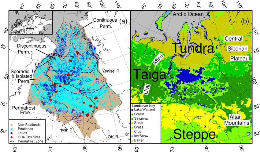
Table 2. Participating models and their relevant hydrologic features.
Model Full name Reference Configuration1 Period Observational constraints on CH4 -producing areas Unsaturated Water table4 Organic Soil
emissions?6 soil7 freeze–
thaw8
Surface Topography3 Maps4 Code5
water2
CLM4Me Community Land Model Riley et al. (2011) CLM4Me 1993–2004 GIEMS – – Sa Yes Uniform Yes Yes
v. 4 Methane
DLEM Dynamic Land Tian et al. (2010, DLEM 1993–2004 GIEMS – – S Yes Uniform No No
Ecosystem Model 2011a, b, 2012)
DLEM2 Dynamic Land Tian et al. (2010, DLEM2 1993–2004 GIEMS – – S Yes Uniform Yes Yes
Ecosystem Model v. 2 2011a,b, 2012)
IAP-RAS Institute of Applied Mokhov et al. IAP-RAS 1993–2004 – – CDIAC M,M+ No n/a Yes Yes
Physics – Russian (2007), NDP017b
Academy of Sciences Eliseev et al.
(2008)
LPJ-Bern Lund-Potsdam- Spahni et al. LPJ-Bern 1993–2004 GIEMS – NCSCD M Yes Uniform Yes Yes
Jena – Bern (2011),
Zürcher et al.
(2013)
LPJ-MPI Lund-Potsdam-Jena – Kleinen et al. LPJ-MPI 1993–2010 – Hydro1Kc – T Yes TOPMODEL Yes No
Max Planck Institute (2012)
LPJ-WHyMe Lund-Potsdam-Jena – Wania et al. LPJ-WHyMe 1993–2004 – – NCSCD M Yes Microtopography Yes Yes
www.biogeosciences.net/12/3321/2015/
Wetland Hydrology (2009a, b; 2010)
and Methane
LPJ-WSL Lund-Potsdam-Jena – Hodson et al. LPJ-WSL 1993–2004 GIEMS – – I No n/a No No
Swiss Federal Institute (2011)
for Forest, Snow,
and Landscape (WSL)
Research
LPX-BERN Land surface Processes Spahni et al. LPX-BERN 1993–2010 GIEMS for – Peregon2008 M,M+ Yes Uniform Yes Yes
and eXchanges – Bern (2013), inundated for peatland
Stocker et al. non-peatland fraction
(2013), wetlands
Stocker et al. LPX-BERN 1993–2010 – ETOPO1d , – T Yes TOPMODEL Yes Yes
(2014) (DyPTOP) Hydro1Kc
LPX-BERN 1993–2010 GIEMS for – Peregon2008 M,M+ Yes Uniform Yes Yes
(N) inundated for peatland
non-peatland fraction
wetlands
LPX-BERN 1993–2010 – ETOPO1d , – T Yes TOPMODEL Yes Yes
(DyPTOP-N) Hydro1Kc
ORCHIDEE Organizing Carbon and Ringeval et al. ORCHIDEE 1993–2004 GIEMS Hydro1Kc – Sa Yes TOPMODEL Yes Yes
Hydrology in Dynamic (2010)
Ecosystems
T. J. Bohn et al.: Intercomparison of wetland methane emissions models
SDGVM Sheffield Dynamic Hopcroft et al. SDGVM 1993–2004 – ETOPO 2v2e – T Yes Uniform No No
Global Vegetation (2011)
Model
UW-VIC Variable Infiltration Bohn et al. UW-VIC 1993–2004 GIEMS SRTMf , Sheng2004 M,M+ Yes Microtopography Yes Yes
Capacity – University of (2013) (GIEMS) ASTERg
Washington
UW-VIC 1993–2010 SWAMPS SRTMf , Sheng2004 M,M+ Yes Microtopography Yes Yes
(SWAMPS) ASTERg
VIC-TEM- Variable Infiltration Zhu et al. (2014) VIC-TEM- 1993–2004 GIEMS Hydro1Kc T Yes TOPMODEL No Yes
TOPMODEL Capacity – Terrestrial TOPMODEL
Ecosystem Model –
TOPography based
hydrologic MODEL
VISIT Vegetation Integrative Ito and VISIT 1993–2010 – – GLWD M,M+ Yes Uniform No No
SImulator for Inatomi (2012) (GLWD)
Trace gases
VISIT 1993–2010 – – Sheng2004 M,M+ Yes Uniform No No
(SHENG)
VISIT 1993–2010 – – GLWD M,M+ Yes Uniform No No
(GLWD-WH)
VISIT 1993–2010 – – Sheng2004 M,M+ Yes Uniform No No
(SHENG-WH)
1 Configuration: short name identifying both the model and the parameter or feature settings for a particular simulation; for models that contributed only a single simulation, the configuration equals the model name.
2 Surface water: name of time-varying surface water product (if any) used as a constraint on CH -contributing area.
4
3 Topography: name of topographic product (if any) used as a constraint on CH -contributing area.
4
4 Map: Name of static wetland map product (if any) used as a constraint on CH -contributing area.
4
5 Code: single-letter code summarizing the types of CH -contributing area constraints used (S: surface water only; T: topography with or without surface water constraint; M: static wetland map with or without surface water or topography constraints; M+: subset of M that excludes the NCSCD).
4
6 Water table: approach used to account for water table depths (uniform: water table depth is the same at all wetland points within the grid cell; TOPMODEL: water table depth varies spatially within the grid cell as a function of topography, following a TOPMODEL approach (Beven and Kirkby, 1979); microtopography:
water table depth varies spatially within the grid cell as a function of assumed microtopography; n/a: not applicable).
7 Soil freeze–thaw: yes or no indicates whether the model accounts for the freezing and thawing of water within the soil column.
Biogeosciences, 12, 3321–3349, 2015
3327
a CLM4Me and ORCHIDEE are listed as S due to tuning or rescaling of inundated areas to match GIEMS, thus destroying contribution of topography.
b http://cdiac.esd.ornl.gov/ndps/ndp017.html, c Hydro1K (2013), d Amante and Eakins (2009), e ETOPO (2006), f Farr et al. (2007), g NASA (2001).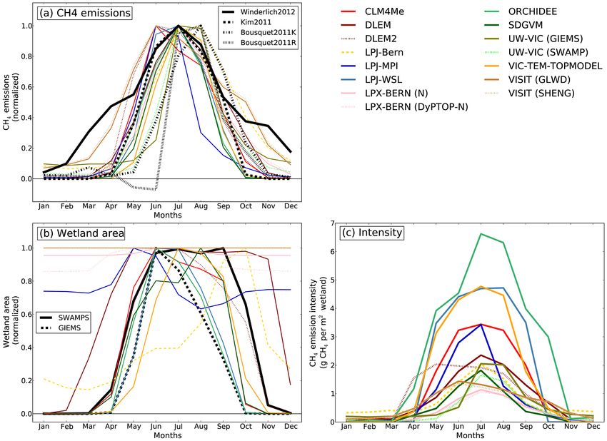
3328                                             T. J. Bohn et al.: Intercomparison of wetland methane emissions models

and “VISIT (GLWD-WH)” and “VISIT (Sheng-WH)” re-                and ORCHIDEE tied their surface water areas to the long-
placed the Cao model with the Walter and Heimann (2000)         term mean of GIEMS: CLM4Me did so by calibration and
model. LPX-BERN (Spahni et al., 2013; Stocker et al., 2013,     ORCHIDEE did so by rescaling its surface water areas. Thus,
2014) is a newer version of LPJ-Bern that also contributed      we have placed these two models in the S category in Table 2.
four configurations: “LPX-BERN”, which prescribed peat-            Finally, the remaining models (IAP-RAS, LPJ-Bern, LPJ-
land extent using Peregon2008 and inundation extent using       WHyMe, LPX-BERN, LPX-BERN (N), both UW-VIC con-
GIEMS; “LPX-BERN (DyPTOP)”, which dynamically pre-              figurations, and all four VISIT configurations) used wetland
dicted the extents of peatlands and inundation; and “LPX-       maps, either alone or in combination with topography and
BERN (N)” and “LPX-BERN (DyPTOP-N)”, which addi-                surface water products, to inform their wetland schemes;
tionally simulated interactions between the carbon and ni-      these are denoted by “M” in Table 2. In most cases, the wet-
trogen cycles. DLEM2 is a newer version of DLEM that in-        land maps were used to determine the maximum extent of the
cludes soil thermal physics and lateral matter fluxes (Liu et   CH4 -producing area, within which inundated area and wa-
al., 2013; Pan et al., 2014). LPJ-MPI (Kleinen et al., 2012)    ter table depths would vary in time. In contrast, LPJ-Bern,
is a version of the LPJ model that contains a dynamic peat-     LPX-BERN, and LPX-BERN (N) allowed inundated area
land model with methane transport by the model of Walter        (specified by GIEMS) to sometimes exceed the static map-
and Heimann (2000). Finally, VIC-TEM-TOPMODEL (Zhu              based peatland area; in such cases, it was assumed that the
et al., 2014) is a hybrid of UW-VIC (Liang et al., 1994), TEM   excess inundation occurred in mineral soils. Thus, the CH4 -
(Zhuang et al., 2004), and TOPMODEL (Beven and Kirkby,          producing area included peatlands and inundated mineral
1979).                                                          soils. LPJ-Bern additionally allowed CH4 production in ar-
   The relevant hydrologic and biogeochemical features of       eas of “wet mineral soil” (in which soil moisture content was
these models are listed in Tables 2 and 3, respectively.        greater than 95 % of water-holding capacity) and included
The models used a variety of approaches to define CH4 -         this in the total CH4 -producing area.
producing areas. To have some consistency across models,           Models’ hydrologic approaches varied in other ways as
the original WETCHIMP study asked participating mod-            well. Some (IAP-RAS and LPJ-WSL) did not include ex-
elers to use the GIEMS product if their model required          plicit water table depth formulations for estimating emis-
wetland extent to be prescribed. Accordingly, some models       sions in unsaturated (non-inundated) wetlands; IAP-RAS as-
(DLEM, DLEM2, and LPJ-WSL) used the GIEMS surface               sumed all wetlands were completely saturated, and LPJ-
water product exclusively to prescribe (time-varying) CH4 -     WSL only considered unsaturated wetlands implicitly, using
producing areas; these are denoted by the code “S” in Ta-       soil moisture as a proxy. Most of the other models used a
ble 2.                                                          TOPMODEL approach to relate the distribution of water ta-
   Several models (CLM4Me, LPJ-MPI, LPX-BERN (DyP-              ble depths across the grid cell to topography (generally on
TOP), LPX-BERN (DyPTOP-N), ORCHIDEE, SDGVM,                     a 1 km scale). However, LPJ-WHyMe, UW-VIC (GIEMS),
and VIC-TEM-TOPMODEL) predicted surface water and               and UW-VIC (SWAMPS) determined water table depth dis-
CH4 -producing areas dynamically using topographic infor-       tributions within peatlands from assumed proportions of mi-
mation and the TOPMODEL (Beven and Kirkby, 1979) dis-           crotopographic landforms (e.g., hummocks and lawns) on
tributed water table approach (in which the area over which     the (horizontal) scale of meters. UW-VIC explicitly handled
the water table is at or above the soil surface can be inter-   lakes by treating lakes and peatlands as a single system, span-
preted to correspond to surface water extent); these mod-       ning the total area of lakes and peatlands which was given by
els are denoted by a “T” in Table 2. For these models, the      the Sheng et al. (2004) data set and within which surface wa-
CH4 -producing area is the area in which labile soil carbon     ter area varied dynamically. Areas of permanent surface wa-
is sufficiently warm and anoxic for methanogenesis to oc-       ter over the period 1949–2010 were considered to be lakes
cur, including both surface water and any non-inundated land    and were excluded from methane emissions estimates.
with sufficiently shallow water table depths. LPJ-MPI and          Models also varied in their soil thermal physics schemes.
LPX-BERN (DyPTOP and DyPTOP-N) prognostically de-               Most models used a one-dimensional heat diffusion scheme
termined peatland area as a function of long-term soil mois-    to determine the vertical profile of soil temperatures, but
ture conditions; their CH4 -producing areas thus included       VISIT used a linear interpolation between current air tem-
peatlands (inundated or not) as well as completely saturated    perature (at the soil surface) and annual average air tem-
or inundated mineral soils. Because the other T models’         perature (at the bottom of the soil column). Several mod-
CH4 -producing areas had no explicit limits, those teams re-    els (DLEM, LPJ-MPI, LPJ-WSL, and SDGVM) did not con-
ported approximations of the models’ true CH4 -producing        sider the water-ice phase change and therefore did not model
areas: CLM4Me, ORCHIDEE, and VIC-TEM-TOPMODEL                   permafrost. While IAP-RAS contained a permafrost scheme,
reported their surface water areas; and SDGVM reported the      it was driven by seasonal and annual summaries of meteo-
area for which the water table was above a threshold depth,     rological forcings and used simple analytic functions to esti-
with the threshold chosen to minimize the global rms error      mate the seasonal evolution and vertical profile of soil tem-
between this area and GIEMS. Additionally, both CLM4Me          peratures. Additionally, DLEM and LPJ-WSL did not con-

Biogeosciences, 12, 3321–3349, 2015                                                 www.biogeosciences.net/12/3321/2015/
T. J. Bohn et al.: Intercomparison of wetland methane emissions models 3329
Table 3. Participating models and their relevant biogeochemical features.
Model 1
Ranaerobic /Raerobic C substrate source2 pH3 Redox Dynamic Nitrogen–carbon Saturated NPP Parameter selection8
state4 vegetation5 cycle interaction6 inhibition7
CLM4Me Variable Cpool Yes Yes Yes Yes No Optimized to various sites
DLEM Variable NPP and Cpool Yes Yes No No No Optimized to various sites
DLEM2 Variable NPP and Cpool Yes Yes No No No Optimized to various sites
IAP-RAS n/a Cpool No No No No No Literature; scaled to global total
LPJ-Bern Constant NPP and Cpool No No Yes No Yes Optimized to various sites;
scaled to global total
LPJ-MPI Constant Cpool No No Yes No Yes Literature
LPJ-WHyMe Constant NPP and Cpool No No Yes No Yes Literature; scaled to global total
LPJ-WSL Constant Cpool No No Yes No No Literature
LPX-BERN Constant NPP and Cpool No No Yes No Yes Optimized to various sites;
scaled to global total
LPX-BERN (DyPTOP) Constant NPP and Cpool No No Yes No Yes Optimized to various sites;
scaled to global total
LPX-BERN (N) Constant NPP and Cpool No No Yes Yes Yes Optimized to various sites;
scaled to global total
LPX-BERN (DyPTOP-N) Constant NPP and Cpool No No Yes Yes Yes Optimized to various sites;
scaled to global total
ORCHIDEE Variable Cpool No No Yes No No Literature and optimized to
various sites
SDGVM Variable Cpool No No Yes No No Literature
UW-VIC(GIEMS) Variable NPP No No No No Yes Optimized to sites in
Glagolev2011
UW-VIC(SWAMPS) Variable NPP No No No No Yes Optimized to sites in
Glagolev2011
VIC-TEM-TOPMODEL Variable NPP Yes Yes No No No Optimized to various sites
VISIT(GLWD) Variable Cpool No No No Yes (only affects No Literature
upland CH4 oxidation)
VISIT(GLWD-WH) Variable NPP No No No Yes (only affects No Literature
upland CH4 oxidation)
VISIT(Sheng) Variable Cpool No No No Yes (only affects No Literature
upland CH4 oxidation)
VISIT(Sheng-WH) Variable NPP No No No Yes (only affects No Literature
upland CH4 oxidation)
1R
anaerobic /Raerobic : how the ratio of anaerobic to aerobic respiration is handled in the model (constant: ratio is held constant; variable: ratio varies either as an explicit function of environmental conditions or as the result of separate governing equations for aerobic
and anaerobic respiration; n/a: not applicable).
2 Carbon substrate source: Cpool: soil carbon pool; NPP: root exudates, in proportion to net primary productivity.
3 pH: indicates whether soil pH influences CH emissions.
4
4 Redox state: indicates whether soil redox state influences CH emissions.
4
5 Dynamic vegetation: indicates whether vegetation species abundances change in response to environmental conditions.
6 Nitrogen–carbon cycle interaction: indicates whether interactions between the nitrogen and carbon cycles influence CH emissions.
4
7 Saturated NPP inhibition: indicates whether NPP decreases under wet soil conditions for any plant species.
8 Parameter selection: method of choosing parameter values (literature: values chosen from ranges reported in literature; optimized: values chosen to minimize the difference between simulated and observed values, either of CH fluxes at selected sites or of global
4
atmospheric CH4 concentrations).
sider the insulating effects of organic (peat) soil. In contrast, SDGVM, VISIT (GLWD), and VISIT (Sheng)) related car-
UW-VIC modeled permafrost, peat soils, and the dynamics bon substrate to the content and residence times of various
of surface water, including lake ice cover and evaporation, soil carbon reservoirs; and others (DLEM, DLEM2, LPJ-
thereby adding another factor that influences soil tempera- Bern, LPJ-WHyMe, all four LPX-BERN configurations)
tures. drew carbon substrate from a combination of both root ex-
Models also varied in their biogeochemical schemes (Ta- udates and soil carbon (or dissolved organic carbon, in the
ble 3). Most represented methane production as a func- case of DLEM and DLEM2). CLM4Me and two configu-
tion of soil temperature, water table depth (except for IAP- rations of LPX-BERN simulated interactions between the
RAS and LPJ-WSL), and the availability of carbon sub- carbon and nitrogen cycles. Several models (all versions of
strate. Most (except for IAP-RAS and LPJ-WSL) explic- LPJ and LPX, ORCHIDEE, and SDGVM) included dynamic
itly accounted for the oxidation of methane above the wa- vegetation components. Some models (LPJ-Bern, LPJ-MPI,
ter table; and most accounted for some degree of plant-aided LPJ-WHyMe, LPX-BERN, and UW-VIC) accounted for the
transport. Some models (LPJ-Bern, LPJ-MPI, LPJ-WHyMe, inhibition of NPP of some plant species under saturated soil
and LPX-BERN) represented methane production as either a moisture conditions. Finally, models employed a variety of
constant or soil-moisture-dependent fraction of aerobic res- methods, alone or in combination (Table 3), to select param-
piration. Some models (DLEM, DLEM2, and VIC-TEM- eter values, including taking the median of literature values,
TOPMODEL) imposed additional dependences on soil pH optimizing emissions to match in situ observations from rep-
and oxidation state. Models differed in the pathways and resentative sites regionally (e.g., UW-VIC optimized param-
availability of carbon substrate: some models (UW-VIC, eter values to match the Glagolev2011 data set in the WSL)
VIC-TEM-TOPMODEL, VISIT (GLWD-WH), and VISIT or globally, or optimizing global total emissions to match var-
(Sheng-WH)) related carbon substrate availability to net pri- ious estimates from inversions.
mary productivity (NPP) as a proxy for root exudates; some
(CLM4Me, IAP-RAS, LPJ-MPI, LPJ-WSL, ORCHIDEE,
www.biogeosciences.net/12/3321/2015/ Biogeosciences, 12, 3321–3349, 2015
3330                                                   T. J. Bohn et al.: Intercomparison of wetland methane emissions models

Figure 2. Mean annual emissions from the WSL: from inversions (green), observation-based estimates (red), and forward models (blue). The
hatched portions of the bars indicate the emissions from the southern half of the domain (latitude < 61◦ N). Error bars on the model results
indicate the interannual standard deviations of the southern and northern emissions. Error bars on the inversions and observational estimates
indicate the uncertainty given in those studies. Numeric fractions of the total emissions contributed by the southern and northern halves of
the domain are displayed in the right-hand column.

2.5    Model simulations                                                 2.6    Data access

                                                                         All data used in this study, including observational products,
To be consistent with WETCHIMP’s transient simulation                    inversions, and forward model results, are available from
(“Experiment 2-trans”, Wania et al., 2013), we focused our               WETCHIMP-WSL (2015).
analysis on the period 1993–2004, although several non-
WETCHIMP models provided data from 1993–2010. All
models used the CRUNCEP gridded meteorological forcings                  3     Results
(Viovy and Ciais, 2011) as a common input. Model-specific
inputs are described in Wania et al. (2013).                             3.1    Average annual total emissions
   Model outputs (monthly CH4 emissions (average g CH4
month−1 m−2 over the grid cell area) and monthly CH4 -                   As shown in Fig. 2 and Table S1 in the Supple-
producing area (km2 )) were analyzed at a 0.5◦ × 0.5◦ spatial            ment, 12-year mean estimates (±standard error on
resolution (resampled from native resolution as necessary).              the mean) of annual total emissions over the WSL
   Due to large seasonal variations in CH4 -producing areas,             from forward models (5.34 ± 0.54 Tg CH4 yr−1 ), in-
our analysis focused on June–July–August (JJA) averages of               versions (6.06 ± 1.22 Tg CH4 yr−1 ), and observations
area and CH4 emissions, since it is during these months that             (3.91 ± 1.29 Tg CH4 yr−1 ) largely agreed, despite large
the majority of the year’s methane is emitted across all mod-            scatter in individual estimates. Model estimates ranged
els (areas in other seasons would not be representative of               from 2.42 (LPX-BERN (DyPTOP-N)) to 11.19 Tg CH4 yr−1
annual CH4 emissions). Similarly, in analyzing interannual               (IAP-RAS). The Glagolev2011 estimate was substantially
variability in CH4 emissions, we focused on JJA CH4 emis-                lower than the mean of the models, corresponding to the
sions, which dominate the annual total and have stronger cor-            36th percentile of the distribution of model estimates.
relations with JJA environmental factors (such as air temper-            However, the potential upward revision of Glagolev2011
ature, precipitation, or inundation) than annual CH4 emis-               (Sect. 2.2) would move it to a substantially higher percentile
sions have with annual average environmental factors. We                 of their distribution. Inversions yielded a similarly large
also computed growing season CH4 “intensities” (average                  range of estimates: 3.08 (Kim2011) to 9.80 Tg CH4 yr−1
JJA CH4 emissions per unit JJA CH4 -producing area).                     (Winderlich2012). Despite their large spread, 15 out of

Biogeosciences, 12, 3321–3349, 2015                                                            www.biogeosciences.net/12/3321/2015/
T. J. Bohn et al.: Intercomparison of wetland methane emissions models 3331
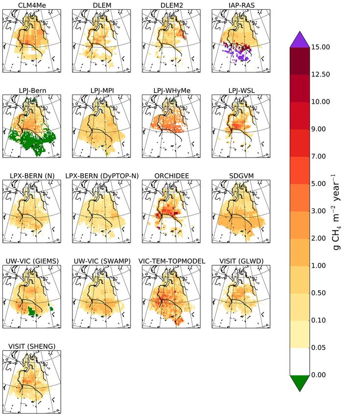
Figure 3. Observational data sets related to wetland areas. For SWAMPS and GIEMS, areas shown are the June–July–August (JJA) average
surface water area fraction over the period 1993–2004.
the 17 forward models fell within the range of inversion 70◦ E), and north of the Ob’ River (61–66◦ N, 70–80◦ E). In
estimates. Here we have excluded the “WH” configurations comparison, the GLWD map entirely lacks wetlands in the
of VISIT and the configurations of LPX-BERN for which tundra region north of 67◦ N and shows additional wetland
nitrogen–carbon interaction was turned off, due to their area in the northeast (64–67◦ N, 70–90◦ E). The NCSCD is
similarities to their counterparts that were included. The substantially different from the other three maps. Owing to
wide variety in the relative proportions of CH4 emitted from its focus on permafrost soils, it completely excludes the ex-
the south and north halves of the domain, with the southern tensive wetlands south of the southern limit of permafrost
contribution ranging from 13 to 69 % (right-hand column (approximately 60◦ N). Given the numerous field studies
in Fig. 2), indicates a lack of agreement on which types of documenting these productive southern wetlands (Sect. 2.1),
wetlands and climate conditions are producing the bulk of the NCSCD seems to be inappropriate for studies that extend
the region’s CH4 . beyond permafrost.
The two surface water products (GIEMS and SWAMPS)
3.2 Differences among observational data sets also exhibit large differences. While they both agree that the
surface water area fraction (Fw ) is most extensive in the cen-
The large degree of disagreement among observational data tral region north of the Ob’ River (61–64◦ N), GIEMS gives
sets is worth addressing before using them to evaluate the areal extents that are 3–6 times those of SWAMPS. Outside
models. Important differences are evident among wetland of this central peak, GIEMS Fw drops off rapidly to nearly 0
maps (Fig. 3). Sheng2004 and Peregon2008 are extremely in most places (particularly in the forested region south of the
similar, in part because they both used the map of Ro- Ob’ River, which may be due to difficulties in detecting in-
manova (1977) north of 65◦ N. Both of these data sets show undation under vegetative canopy and/or reduced sensitivity
wetlands distributed across most of the WSL, with large con- where the open-water fraction is less than 10 %; Prigent et al.,
centrations south of the Ob’ River (55–61◦ N, 70–85◦ E), east 2007), while SWAMPS maintains low levels of Fw through-
of the confluence of the Ob’ and Irtysh rivers (57–62◦ N, 65–
www.biogeosciences.net/12/3321/2015/ Biogeosciences, 12, 3321–3349, 20153332 T. J. Bohn et al.: Intercomparison of wetland methane emissions models
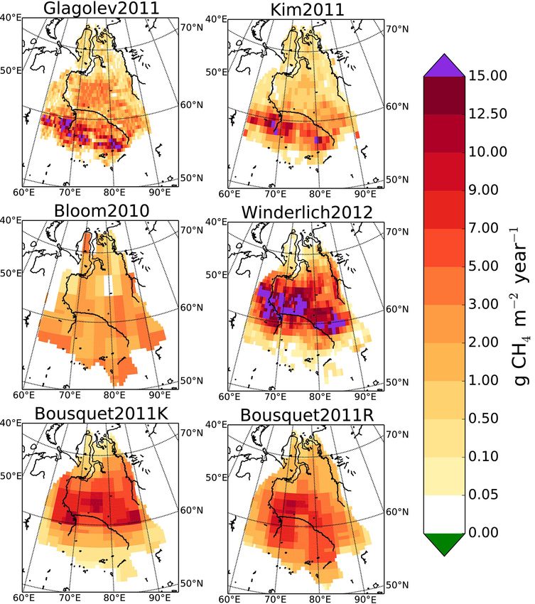
Figure 4. Observation- and inversion-based estimates of annual CH4 emissions (g CH4 yr−1 m−2 of grid cell area). For inversions, averages
are over the following periods: 2002–2007 (Kim2011), 2003–2007 (Bloom2010), 2009 (Winderlich2012), and 1993–2004 (Bousquet2011K
and R).
out most of the WSL. Along the Arctic coastline, SWAMPS tle spatial variability in emissions, likely due to its use of
shows high Fw , which may indicate contamination of the sig- GRACE observations as a proxy for wetland inundation and
nal by the ocean. In both data sets, Fw exhibits some similar- water table conditions.
ity with the distribution of lakes and rivers (Fig. 1), illus-
trating the inclusion of non-wetlands in these surface water 3.3 Primary drivers of model spatial uncertainty
products.
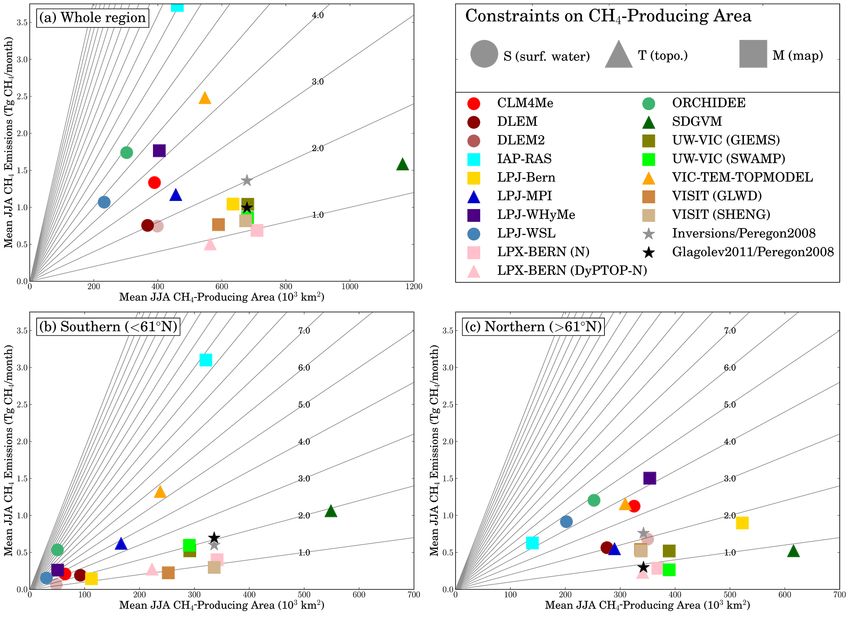
Among the CH4 data sets (Fig. 4), a clear difference can be The wide disagreement among models is plainly evident in
seen between the spatial distributions of Glagolev2011 and Fig. 5, which plots average JJA CH4 emissions versus aver-
Kim2011 (both of which assign the majority of emissions to age JJA CH4 -producing areas for the WSL as a whole (top
the region south of the Ob’ River, between 55 and 60◦ N); left), the south (bottom left), and the north (bottom right).
and Winderlich2012 and Bousquet2011K (both of which as- A series of lines (“spokes”) passing through the origin, with
sign the majority of emissions to the central region north of slopes of integer multiples of 1 g CH4 m−2 month−1 , allows
the Ob’ River, between 60 and 65◦ N). We discuss possible comparison of spatial average intensities (CH4 emissions per
reasons for this discrepancy in Sect. 4.3. The global inver- unit CH4 -producing area). All points along a given line have
sions (Bousquet2011R and K, and Bloom2010) have coarser the same intensity but different CH4 -producing areas. We
spatial resolution than the regional inversions of Kim2011 have included the Glagolev2011–Peregon2008 CH4 –area es-
and Winderlich2012. Bousquet2011R and K have similar timate (denoted by a black star) and the mean of the inver-
distributions between 60 and 65◦ N, but Bousquet2011R sions (denoted by a grey star) for reference. We set the area
has relatively stronger emissions between 57 and 60◦ N and coordinate for the inversions to Peregon2008 because (a) the
weaker emissions between 65 and 67◦ N; in this respect, wetland area was not available for all inversions and (b) Pere-
Bousquet2011R is intermediate between Glagolev2011 and gon2008 is a relatively accurate estimate of wetland area. JJA
Winderlich2012. Finally, Bloom2010 exhibits relatively lit- CH4 emissions, JJA wetland or CH4 -producing areas, and
JJA intensities, for all models, observations, and inversions,
Biogeosciences, 12, 3321–3349, 2015 www.biogeosciences.net/12/3321/2015/T. J. Bohn et al.: Intercomparison of wetland methane emissions models 3333
Figure 5. Model estimates of JJA CH4 emissions (Tg CH4 month−1 ) and JJA wetland or CH4 -producing area (103 km2 ): for the entire WSL
(top left) and the southern (bottom left) and northern (bottom right) halves, for the period 1993–2004. Lines passing through the origin,
with slopes of integer multiples of 1 g CH4 m−2 month−1 , allow a comparison of spatial average intensities (CH4 emissions per unit CH4 -
producing area). Circles denote models that used satellite surface water products alone (corresponding to code S in Table 2) to delineate
wetlands. Triangles denote models that used topographic information, with or without surface water products (corresponding to code T in
Table 2). Squares denote models that used wetland maps with or without topography or surface water products (corresponding to code M in
Table 2).
Table 4. Estimates of June–July–August CH4 emissions from subsets of the participating models, over the entire WSL and its southern
(< 61◦ N) and northern halves, for the period 1993–2004. Biases were computed with respect to the Glagolev2011–Peregon2008 estimates.
Subset Average Jun–Jul–Aug CH4 (Tg CH4 month−1 ) Average Jun–Jul–Aug contributing area (103 km2 )
WSL South North WSL South North
Mean Bias SD Mean Bias SD Mean Bias SD Mean Bias SD Mean Bias SD Mean Bias SD
I 1.10 0.14 0.37 0.22 −0.45 0.16 0.89 0.59 0.24 388 −291 136 66 −270 31 321 −21 112
T 1.42 0.46 0.82 0.81 0.14 0.46 0.61 0.31 0.39 682 4 325 294 −42 173 389 46 153
M 1.32 0.36 1.01 0.69 0.02 0.97 0.64 0.34 0.40 605 −74 113 250 −87 109 355 12 105
M+ 1.30 0.34 1.17 0.85 0.18 1.10 0.45 0.16 0.15 633 −46 93 306 −30 34 327 −15 95
are listed in Table S1. Over the entire WSL (Fig. 5, top left), estimates is substantially skewed, with most models’ esti-
the scatter in model estimates of CH4 emissions results from mates falling well below both Glagolev2011 and the mean
scatter in both area (ranging from 200 000 to 1200 000 km2 ) of the inversions. Glagolev2011’s estimate corresponds to
and intensity (ranging from 1 to 8 g CH4 m−2 month−1 ), with the 81st percentile of the model CH4 distribution; the ex-
no clear relationship between the two. pected upward revision of Glagolev2011 (Sect. 2.2; exact
However, a strong area-driven bias is evident in the south JJA amount not yet known) would only raise that percentile.
(Fig. 5, bottom left). Although the mean modeled CH4 emis- The mean of the inversions corresponds to the 76th per-
sion rate (0.58 Tg CH4 month−1 ) is fairly close to both centile. Similarly, the models substantially underestimate
Glagolev2011 (0.67 Tg CH4 month−1 ) and the mean of in- the CH4 -producing area, with Peregon2008 occupying the
versions (0.60 Tg CH4 month−1 ), the distribution of model 83rd percentile of the model distribution. On the other hand,
www.biogeosciences.net/12/3321/2015/ Biogeosciences, 12, 3321–3349, 2015You can also read