Greenhouse Gas Emission Inventory Sonoma County, California - for all sectors of January 2005 Bay Area Air Quality Management District Sonoma ...
←
→
Page content transcription
If your browser does not render page correctly, please read the page content below

Greenhouse Gas Emission Inventory
                for all sectors of

    Sonoma County, California

                 January 2005

                 Prepared for the

    Bay Area Air Quality Management District
                     and the

   Sonoma County Waste Management Agency
                      by the

          Climate Protection Campaign
Greenhouse Gas Emission Inventory
for all sectors of Sonoma County, California
January 2005
Abstract
This report,1 funded by the Bay Area Air Quality Management District, describes the results of
the greenhouse gas emissions inventory for all sectors of Sonoma County. This represents
Sonoma’s first community-wide climate protection effort, and the first climate protection
initiative undertaken by a California regional air district. This report is intended to help Sonoma
County governments, businesses, and residents reduce their greenhouse gas emissions. Also it
aims to inspire other communities to conduct similar inventories, and guide them as they do so.
The following tasks and findings correspond to the study’s scope of work.
A. Inventory Sonoma County’s greenhouse gases (GHG)
For the inventory we reviewed the science of global climate change, and the relationship
between greenhouse gas emissions and criterion air pollutants. We followed emission accounting
protocol from Cities for Climate Protection, and categorized emissions into four sectors:
• Electricity and natural gas
• Vehicular transportation
• Agriculture
• Solid waste
We found that from 1990 to 2000, Sonoma County’s GHG emissions increased overall by 28
percent. Key factors for this rise are an increase in vehicle miles traveled of 42.5 percent, and an
increase in population of 18 percent.
B. Recommend emission reduction targets
Scientists say that we need to reduce emissions of carbon dioxide, the major GHG, by 50 to 70
percent to stabilize its concentration in the atmosphere, and can succeed in making such
reductions using solutions that exist today. After surveying options for GHG reduction targets,
we recommend that Sonoma County adopt a 20 percent reduction from 1990 levels by 2010, a
bold beginning to align this area’s GHG emissions with the scientific imperative.
C. Recommend next steps
We recommend that Sonoma County launch an initiative through which representatives from
diverse sectors of the community come together to consider and adopt GHG emissions reduction
targets; and create, adopt, and commit to implementing a plan for reaching the target.
1
This report is posted at www.climateprotectioncampaign.org
2
Greenhouse Gas Emission Inventory
        for all sectors of Sonoma County, California
                                                      January 2005

                                           Table of Contents
                                                                                                                                  Page
A. Greenhouse gas emission inventory for all sectors of Sonoma County.............                                                  4
     Project background and overview............................................................................                    4
     Project work statement.............................................................................................            5
     Global climate change
          Description and significance...............................................................................               6
          Types and strengths of greenhouse gases...........................................................                        7
          Relationship between global climate change and air quality..............................                                  9
     Summary of findings................................................................................................           12
     Greenhouse gas emission accounting......................................................................                      14
     Sectors
          Electricity and natural gas...................................................................................           15
          Transportation.....................................................................................................      19
          Agriculture..........................................................................................................    22
          Solid waste..........................................................................................................    27
     Marin, San Francisco, Sonoma comparison............................................................. 31
     California context.....................................................................................................       33
B. Recommendations for emission reduction targets for Sonoma County............                                                    36
     Choices for the future...............................................................................................         38
C. Recommendations for next steps for reducing GHG emissions in Sonoma
   County.....................................................................................................................     40
     Examples of emission reduction measures..............................................................                         42
     Resources.................................................................................................................    47
D. Highlights of stakeholder meetings....................................................................... 50
E. Press coverage for the project...............................................................................                   53
Acknowledgments........................................................................................................            55

                                                                  3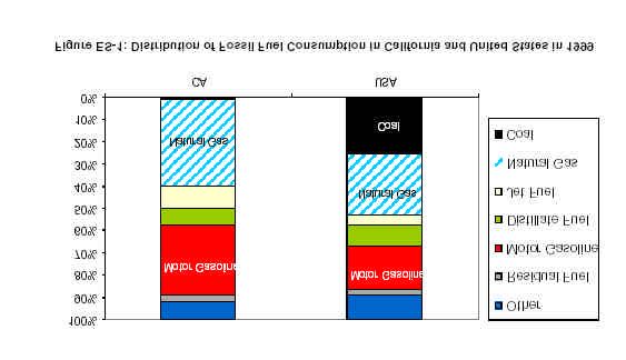
A. Greenhouse gas emission inventory for
   all sectors of Sonoma County, California

Project background and overview
In August 2002, Sonoma became the first county in the nation where 100 percent of its
municipalities—the County and all nine cities—pledged by resolution to measure and reduce
their greenhouse gas (GHG) emissions. They joined Cities for Climate Protection®, a campaign
led by ICLEI - Local Governments for Sustainability. Over 600 communities participate in this
campaign worldwide, with over 150 of them in the U.S.

The Cities for Climate Protection (CCP) program consists of five milestones:
       Milestone One:         Inventory greenhouse gas emission production
       Milestone Two:         Set a target for emission reduction
       Milestone Three:       Create a plan for meeting the target
       Milestone Four:        Implement the plan
       Milestone Five:        Monitor progress and adjust as appropriate

Municipalities can focus on GHG emissions produced by their internal operations, on emissions
produced by all sectors in the jurisdiction, or first one and then the other. Sonoma municipalities
chose to “lead by example,” focusing on internal operations first. This study represents
Sonoma’s first assessment of the greenhouse gas emitted by the whole community.

The County of Sonoma and the City of Santa Rosa completed their GHG emissions
inventories—Milestone One—for their internal operations in 2002. The County also set a
target—Milestone Two—to reduce the emissions produced by its internal operations by 20%
from 2000 to 2010. The remaining eight Sonoma cities completed inventories of the emissions
produced by their internal operations in September 2003.2 In doing so, Sonoma set a second
national precedent when 100 percent of its municipalities completed their baseline emission
inventories. In 2004, Rohnert Park, Sebastopol, and Cotati set their emission reduction targets –
Milestone Two - for their internal operations. All three cities’ targets are the same as the
County’s except Sebastopol’s which is 30% from 2000 by 2008.

In 2002 the Sonoma County Mayors’ and Council members’ Association sent a letter to the
Chair of the Board of the Bay Area Air Quality Management District encouraging the district to
support climate protection. In June 2003, the Air District Board approved a request for financial
support of a two-part study comprised of a GHG inventory for all sectors of Sonoma County, and
research regarding actions underway regionally and nationwide in which air quality and climate
protection efforts are being integrated. The Sonoma County Waste Management Agency served
as administrator for the study.

2
    References for inventory reports are listed under Resources, page 47.

                                                                  4
This report of Sonoma County’s emissions inventory is intended for use by other communities as
an example of how to inventory their GHG emissions. The report on the second part of the study,
Phase 2, will be issued separately.
Project work statement
Phase 1. Inventory of the greenhouse gases emitted in Sonoma County
Task Description Corresponding
CCP Milestone
A. Analysis: Inventory of Greenhouse gas emission inventory for Sonoma County broken down Milestone One –
GHG emissions into at least three sources – residential, business, and governmental. Inventory
B. Recommendations: Recommendations for GHG emission reduction targets for Sonoma Milestone Two –
Targets County. Target
C. Recommendations: Recommendations for next steps for reducing GHG emissions in Milestone Three -
Next Steps Sonoma County, and how these next steps relate to the BAAQMD’s Plan
Air Quality Plans.
D. Research: Input from A list of the stakeholders involved in producing the inventory report Not applicable
stakeholders with copies of minutes of meetings with stakeholders
E. Public outreach Copies of newspaper articles and other print media coverage, if any, Not applicable
for these efforts listed above.
Phase 2. Integration of air quality and climate protection efforts and the BAAQMD’s role
Task Description
A. Research: District- Inventory of climate protection efforts throughout the Bay Area Air Quality Management
wide inventory District, and identification of the best models for climate protection found in the District.
Description of the coordination, if any, between climate protection and air quality in these
efforts.
B. Research: Nationwide Description of the results of a nationwide review of how climate protection and air quality
review management are being connected and coordinated at the regional level. Identification of the
most effective models for making this connection.
C. Analysis: Relation Analysis of the relation between the BAAQMD’s Air Quality Plans and climate protection
between plans plans, including identification of the overlaps, gaps, and areas of synergy.
D. Recommendations: Model ordinance(s) for local government that addresses and integrate climate protection and
Model ordinance(s) air quality management.
E. Recommendations: Description of a model framework for programs – local, regional, and multi-county – that
Model framework both protect the climate and improve air quality.
F. Recommendations: Description of recommended next steps for the BAAQMD.
Next steps
G. Resources: Possible A list of possible funding sources for climate protection and clean air efforts.
funding sources
H. Resources: Other A list of resources for more information about the above.
I. Research: Source of A list of the stakeholders involved in producing the report with copies of minutes of
information meetings with stakeholders.
J. Final Report A presentation to the BAAQMD Board with the results of the project.
5Global climate change: Description and significance
Heat from the sun is trapped near the Earth’s surface by naturally occurring gases. This
greenhouse effect stabilizes earth’s temperature at an average of approximately 60°F, making
Earth habitable for humankind.
The major greenhouse gas from human activity, carbon dioxide (CO2), is produced when
gasoline, diesel, natural gas, coal and other fossil fuels combust. Methane (CH4), the second
most important greenhouse gas from human activity, is a byproduct of organic decomposition.
As human population and consumption
has increased, so has the amount of
greenhouse gas emitted into Earth’s
atmosphere. In the mid 1850s there was
about 280 parts per million of carbon
dioxide in the atmosphere; now there is
about 379. Human activity has increased
the blanket of heat-trapping gas
surrounding the Earth, magnified the
greenhouse effect, and increased Earth’s
average temperature by an average of
more than 1°F over the last 100 years.
Climate change is caused by a manmade blanket of
Scientists prefer the term climate change carbon dioxide that surrounds the earth and traps in heat.
to global warming because climatic
changes vary across the planet, from
place to place and season to season. With climate change comes extreme weather – both record-
breaking hotter and colder temperatures, both droughts and floods. For example, between 1995
and 1998 there were a record 33 hurricanes in the U.S. In August 2004, Hurricane Charley with
winds of 145 miles per hour in Florida, caused $7.4 billion in damages and killed 27 people. For
many areas in the U.S., droughts in 1998 were among the worst ever. Currently, the western part
of North America is in the midst of one of the worst droughts in 500 years. While no single
weather event can be attributed to global climate change, the pattern of increasing extreme
weather can, say climatologists.
The world’s foremost authority on climate change, the International Panel on Climate Change
(IPCC), involves thousands of scientists worldwide who study atmospheric changes, their
potential impacts, and appropriate policy responses. Having verified the increase in greenhouse
gas, the rise in temperatures, and the impacts on Earth’s living systems, these scientists
concluded that global climate change imperils life on Earth. In 1995, the IPCC specified that
stabilizing the concentration of carbon dioxide required an immediate reduction in CO2 emissions
of 50 to 70 percent, and required further reductions thereafter until the year 2100.3
3
IPCC second assessment synthesis of scientific-technical information relevant to interpreting article 2 of the UN Framework
Convention on Climate Change, 1995, the summary for policymakers, page 9, http://www.ipcc.ch/pub/sa(E).pdf See also
“Climate Change Research - Facts, uncertainties and responses,” Astrid Zwick, Antonio Soria
http://www.jrc.es/pages/iptsreport/vol05/english/art-en1.doc
6Types and strengths of greenhouse gases4
Processes that generate, absorb, and destroy greenhouse gases determine its concentration in the
atmosphere, currently less than 1 percent. Major greenhouse gases besides carbon dioxide and
methane are nitrous oxide (N2O), chlorofluorocarbons (CFCs), and ozone (O3).5 Water vapor
(H2O) also contributes to the greenhouse effect, but human activity has little impact on it,
according to scientists.
The IPCC identified the strength of each type of GHG based on its ability to trap heat, defined as
cumulative radiative forcing.6 Global warming potential also takes into account the atmospheric
lifetimes of GHGs.
Global Warming Potential of major greenhouse gases 7
Greenhouse gas Estimated Lifetime Global Warming Potential
(years)
20 years 100 years 500 years
Carbon Dioxide (CO2) 50-2008 1 1 1
Methane (CH4) 12.0 62 23 7
Nitrous Oxide (N2O) 114 275 296 156
CFCl3 (CFC-11) 45 6300 4600 1600
Chlorofluorocarbons (CFCs)
CF2Cl2 (CFC-12) 100 10200 10600 5200
CClF3 (CFC-13) 640 10000 14000 16300
C2F3Cl3 (CFC-113) 85 6100 6000 2700
C2F4Cl2 (CFC-114) 300 7500 9800 8700
C2F5Cl (CFC-115) 1700 4900 7200 9900
4
Reference: Hong Kong Observatory: http://www.hko.gov.hk/wxinfo/climat/greenhs/e_grnhse.htm Please note that these figures
are from the IPCC’s Third Assessment Report. The protocol followed for this report follows the U.S. inventory as well as the
recommendation of the IPCC, i.e., to continue to use the GWPs from the IPCC’s Second Assessment report through the end of
the first reporting period when inventories will shift over to the Third Assessment Report.
5
Tropospheric ozone concentrations in the Northern Hemisphere may have increased since preindustrial times because of human
activity, resulting in positive radiative forcing. Although not yet well characterized, this forcing is estimated to be about 0.4 Wm2
(15% of that from the long-lived greenhouse gases). However, the observations of the most recent decade show that the upward
trend has slowed significantly or stopped. IPCC Summary for Policy Makers http://www.ipcc.ch/pub/sarsum1.htm
6
Radiative forcing considers the difference between the present and some future time caused by a unit mass of greenhouse gas
emitted now, expressed relative to CO2. Radiative forcing is defined as a change in average net radiation at the top of the
troposphere (tropopause) due to a change in either solar or infrared radiation. A radiative forcing perturbs the balance between
incoming and outgoing radiation. A positive radiative forcing tends on average to warm the Earth's surface; a negative radiative
forcing tends on average to cool the Earth's surface.
7
Global warming potential following the instantaneous injection of 1 Kg of each GHG, relative to 1 Kg of CO2. Table is based on
information found in the IPCC Third Assessment Report, 2001. Derivations of global warming potentials require knowledge of
the fate of the emitted gas (typically not well understood) and the radiative forcing due to the amount remaining in the
atmosphere (reasonably well understood). GWPs typically encompass + 35% uncertainty relative to CO2 reference.
8
Different removal processes result in a varying CO2 lifetime, U.S. Environmental Protection Agency, April 2002,
http://yosemite.epa.gov/oar/globalwarming.nsf/UniqueKeyLookup/SHSU5BUM9T/$File/ghg_gwp.pdf
7Projected changes in global temperature:
Global average 1856-1999 and projection estimates to 2100
Source: Temperatures 1856-1999: Climatic Research Unit, University at East Anglia, Norwich UK. Projection: IPCC report 95.
World Scientists’ Warning to Humanity
Human beings and the natural world are on a collision course. Human activities inflict harsh
and often irreversible damage on the environment and on critical resources. If not checked,
many of our current practices put at serious risk the future that we wish for human society and
the plant and animal kingdoms, and may so alter the living world that it will be unable to
sustain life in the manner that we know. Fundamental changes are urgent if we are to avoid
the collision our present course will bring about.”
--Signed in 1992 by more than 1,600 scientists, including 102 Nobel laureates, from 70 countries
http://www.ucsusa.org/ucs/about/page.cfm:pageID=1009
8Relationship between global climate change and
air quality
The higher temperatures forecast by scientists will worsen air quality in several ways. Ozone
formation tends to increase with higher temperatures, strong sunlight, and a stable air mass, as
shown in the following graph. Higher temperatures also increase air pollution by causing
vegetation to emit more natural hydrocarbon, harder working engines, increases in fuel
evaporation, and greater demands on power plants.9
Recent research confirms that global climate change will likely trigger increases in smog and
health problems even if the level of man-made smog-causing pollutants remains the same. The
research predicts that by 2050 the number of smog-alert days in selected U.S. cities will increase
by about 60%, accompanied by more lung diseases including asthma, more hospital admissions,
and more premature deaths.10
Just as climate change exacerbates air pollution, air pollution also exacerbates climate change.
Incomplete combustion of fossil fuels, biofuels, and biomass produces black carbon, also called
soot or particulate matter. The impact of these air pollutants on global temperature is very
complex.11 Some climate scientists assert that their overall impact is to heat the atmosphere.12
9
“Global Warming and Greenhouse Gas Emissions from Motor Vehicles,” AB 1493 (Pavley) Briefing Package, prepared by the
California Environmental Protection Agency,
http://www.energy.ca.gov/global_climate_change/documents/AB1493_PRESENTATION.PDF
10
“Heat Advisory: How Global Warming causes More Bad Air Days, July 2004,
http://www.nrdc.org/globalWarming/heatadvisory/heatadvisory.pdf
11
“Climate Change Overview: Technical support document for staff proposal regarding reduction of greenhouse gas emissions
from motor vehicles,” California Environmental Protection Agency, Air Resources Board, August 6, 2004,
http://www.arb.ca.gov/cc/factsheets/august_tsd/overview_august.pdf
9Air pollution and climate change share causes and solutions. Reduction in fossil fuel
consumption reduces both criteria pollutants and GHG emissions. Many criteria pollutants,
specifically the various oxides of nitrogen (NOx) produced during combustion originate from
fossil fuel combustion, as does carbon dioxide (CO2), the primary greenhouse gas. Volatile
organic compounds (VOCs) are ozone precursors, and will under certain circumstances, produce
methane. Reducing VOCs improves air quality and helps protect the climate.
Electricity, transportation, and industrial sectors account for most of the U.S. anthropogenic
emissions of criteria pollutants and GHG emissions. Electric and transportation sectors are the
largest aggregate producers of GHG emissions, with each accounting for about 35 percent to 40
percent of total emissions.13 For all sectors, the two essential steps to both clean the air and
protect the climate are improving energy efficiency and switching to lower-carbon or zero-net-
carbon fuels, i.e., renewables.
Enormous opportunities exist worldwide for taking these
essential steps, usually with significant positive economic In continuing to address criteria
benefits as well. For example, estimates from the Centre pollutant nonattainment
for Integrated Assessment Modelling indicate that Kyoto- challenges, state and local
level cuts in CO2 emissions would reduce the cost of officials have the opportunity to
reaching European countries’ 2010 air pollution objectives capture significant GHG emission
by at least €5 billion.14 reductions. The most effective
path for achieving this goal is to
Clean air solutions do not necessarily translate to climate ensure that, in obtaining emission
protection. Smog-creating air pollution decreased reductions needed for criteria
substantially in the U.S. following the Clean Air Act of pollutant attainment, the applied
1970. By contrast, CO2 emissions rose during the same strategies are ones that also
period because air quality tactics such as “tailpipe” controls provide GHG reduction benefits,
and smokestack scrubbers have little or no impact on rather than measures that are
carbon dioxide. In fact, some clean air technologies ineffective or counterproductive
actually increase CO2 by lowering plant efficiency, thus from a GHG perspective.
requiring more energy to be used. Some alternative fuels
“Reducing Greenhouse Gases and Air
that are good for air quality either have no effect or Pollution: A Menu of Harmonized
increase GHG emissions. Congestion management Options,” STAPPA /ALAPCO
measures like signal synchronization often reduce
emissions only temporarily. Emissions may actually
increase in the long run because short-term traffic relief encourages people to drive more.
Although strategies that cut standard air pollution often miss GHG emissions, strategies that
reduce GHG emissions almost always improve air quality as well.15
12
See, for example, “Defusing the Global Warming Time Bomb,” James Hansen, Scientific American, March 2004.
13
“Reducing Greenhouse Gases and Air Pollution: A Menu of Harmonized Options,” October 1999, STAPPA/ALAPCO,
http://www.4cleanair.org/comments/execsum.PDF
14
UNECE Convention’s IIASA, http://www.unece.org/env/emep/pr03_env02e_h.pdf
15
“Converging solutions: Clean air and climate protection,” ICLEI fact sheet by Chris Giovinazzo, undated.
10Many initiatives that aim to both clean the air and protect the climate are emerging. One recent
development with potentially far-reaching impacts is the suit filed in July 2004 against five
major utilities by attorneys general from eight states including California, and officials from New
York City. The suit charges that greenhouses gas emissions from the utility companies are
creating a public nuisance. The suit seeks a court order to require the utilities to reduce these
emissions. Attorneys general contend that they must act because normal regulatory approaches
such as action from the E.P.A., Congress, and the administration, have failed to adequately
address the threat posed by utilities’ GHG emissions.16
Passage of AB1493 in 2002, California’s law to regulate greenhouse gas emissions, represents
the first-ever mandatory reduction of greenhouse gas pollutants from vehicles in the U.S. The
legislation directed the Air Resources Board to develop regulations for automobile
manufacturers to achieve maximum feasible reductions in GHG emissions. In September 2004,
the California Air Resources Board voted unanimously to adopt standards that cut carbon
dioxide emissions by 25 percent starting with the 2009 model year.17
The two major national associations of air pollution control agencies, State and Territorial Air
Pollution Program Administrators (STAPPA) and the Association of Local Air Pollution Control
Officials (ALAPCO) in 1999 issued a substantial education resource guide to help state and local
officials identify and assess harmonized strategies and policies to reduce air pollution and
address climate change simultaneously.18 Also, STAPPA/ALAPCO together with ICLEI in 2003
released software called CACPS – Clean Air and Climate Protection Software – to help state and
local governments track criterion air pollution and GHG emissions.19 CACPS was used for this
Sonoma County GHG emissions inventory.
In Europe, the European Environmental Agency has issued a report that analyzes the linkages
between climate protection and air quality.20
The integration of air quality management and climate protection is the subject of Phase Two of
this project where the relationship between global climate change and air quality from an
implementation and policy perspective will be taken up in more depth.
16
“New environmental cops: state attorneys general,” Christian Science Monitor, July 22, 2004,
http://www.csmonitor.com/2004/0722/p03s01-usju.html
17
“California Goes Ahead With Disputed Smog Plan,” UPI, September 24, 2004, http://www.spacedaily.com/news/pollution-
04c.html
18
“Reducing Greenhouse Gases and Air Pollution: A Menu of Harmonized Options,” October 1999, STAPPA/ALAPCO,
http://www.4cleanair.org/comments/execsum.PDF
19
http://www.cacpsoftware.org
20
http://reports.eea.eu.int/technical_report_2004_5/en/tab_content_RLR
11Summary of findings
This study found that from 1990 to 2000, overall GHG emissions produced in Sonoma County
increased by 28 percent. Two critical factors in this rise are increases in emissions from vehicle
transportation of about 43 percent, and in population of 18 percent during this same period. For
comparison, GHG emissions nationwide increased by 14.2 percent between 1990 and 2000,
according to the U.S. Environmental Protection Agency.21
Greenhouse gas emissions22 (GHG), Sonoma County
1990 2000 % change
GHG % of total GHG % of total
(tons) (tons)
Electricity & 1,430,996 48 1,804,158 47 +26
natural gas
Transportation 1,115,000 37 1,589,000 42 +43
(vehicles only)
Agriculture 444,69023 15 425,040 11 -4
Sub-total 2,990,686 100 3,818,198 100
Solid Waste24 -80,332 -78,818 +2
Total Net GHG 2,910,354 3,739,380 +28
Population 388,222 458,614 +18
GHG per person in
Sonoma 7.5 8.2 +9
21
“Inventory of U.S. Greenhouse Gas Emissions and Sinks: 1990 –2000” U.S. Environmental Protection Agency, 2002,
http://yosemite.epa.gov/oar/globalwarming.nsf/UniqueKeyLookup/SHSU5BUKBK/$File/executive_summary.pdf
22
Greenhouse gas (GHG) is expressed throughout this report, except where otherwise noted, in tons equivalent carbon dioxide
(tons eCO2)
23
Data is for 1992; data for 1990 not available.
24
Solid waste is negative because solid waste’s overall impact is to take GHG out of the atmosphere, following the protocol used
for this inventory. Please see page 27 for an explanation.
124,500,000
Solid Waste
4,000,000 Agriculture
Transportation (vehicles only)
3,500,000 Electricity & Natural Gas
3,000,000
Annual GHG (tons-CO2/yr)
2,500,000
2,000,000
1,500,000
1,000,000
500,000
0
1990 2000
-500,000
13Greenhouse gas emission accounting
Accounting for greenhouse gas emissions, although a relatively new field, has evolved rapidly
over the last ten years as pioneer practitioners worldwide standardize methods and protocols for
calculating GHG emissions. ICLEI – Local Governments for Sustainability, through its Cities for
Climate Protection campaign, is a leader in developing accounting methodology and setting
standards for local communities’ GHG emission inventories. ICLEI coordinates its work with the
California Climate Action Registry,25 the U.S. Department of Energy, the U.S. Environmental
Protection Agency, Canada-based software developers Torrie Smith Associates, and, more
recently, State and Territorial Air Pollution Program Administrators-Association of Local Air
Pollution Control Officials (STAPPA/ALAPCO). As noted previously, over 600 local
governments worldwide participate in ICLEI’s Cities for Climate Protection campaign,
suggesting the importance of having a standard GHG emission protocol, as well as the role
ICLEI plays in promulgating standards.
All accounting methodologies, even in highly advanced fields such as finances, face new
challenges and change over time. GHG accounting is especially challenging, first because of the
relative newness of its methodology, and second because GHG data source development is also
relatively new.
Accounting never exactly represents reality. What is included and excluded is determined by
accounting protocol and by the amount of resources devoted to data collection and analysis. For
example, this GHG inventory doesn’t include emissions from meat consumed locally but
produced elsewhere, nor emissions from residents’ air travel; it does include emissions from
electricity consumed locally even when the electricity is produced elsewhere.
Communities can obtain a good idea of their GHG emissions relatively easily using ICLEI’s
GHG emissions accounting method, as we intend to demonstrate in this report. In general, the
years to be studied are specified, and data - much of it from government sources – is collected
and then converted to greenhouse gas emissions using standard coefficients.
Many communities use software to help organize and convert data into emissions and create
reports. ICLEI and STAPPA/ALAPCO developed and released new software, called Clean Air
Climate Protection Software (CACPS) in 2003 to enable communities to inventory criterion air
pollutants and GHG emissions. CACPS was used for most of the calculations in this study.
Base years chosen for this study, 1990 and 2000, correspond with years for other significant data
benchmarking, i.e., the U.S. Census. The year 2000 also corresponds to the base year used by the
County of Sonoma and Sonoma’s nine cities to inventory GHG emissions of their municipal
operations.
25
The California Climate Action Registry, a non-profit public/private partnership, develops protocols for calculating GHG
emissions, and provides GHG emissions software called CARROT to participating organizations. The Registry anticipates a
carbon trading market in the future, and is now helping businesses establish “credit for early action.” The Registry focuses on
emission tracking and certifying, primarily for business, while ICLEI focuses on a comprehensive climate protection program for
local governments, from pledging to tracking to implementing GHG reduction measures.
14Electricity and natural gas26
Electricity originates with some other form of energy - falling water, wind, geothermal steam,
nuclear, natural gas, oil, or coal. Electricity from fossil fuels emits relatively more greenhouse
gas than electricity from renewable resources, e.g., hydropower, wind, and biomass, as shown in
the following table.27
GHG Power plant
emissions energy source
Hydro, wind, solar Biomass fuels (such as wood) emit carbon dioxide when burned,
Least thermal, biomass but extract carbon dioxide from the atmosphere when they are
growing.
| Geothermal steam contains carbon dioxide which is usually
| Geothermal, solar vented. The production of PV panels is energy intensive;
| photovoltaic (PV), however, if renewable energy sources were used in their
| nuclear manufacture, then GHG emissions would be minimal.
| Electricity is needed to produce enriched uranium nuclear fuel,
| often from coal-powered plants. Waste from nuclear energy
| generation makes this a controversial energy source.
? Natural gas Carbon/Hydrogen Ratio28 (C/H) = 1:4
Most Oil C/H = ~1:2
Coal C/H = ~1:1
Each power plant has its own emissions coefficient that is based on the type of fuel burned and
the plant’s thermal efficiency. Thermal efficiency is a function of the power plant’s design, and
indicates how much of the heat created during combustion becomes electricity. The range for
this is about 30 to 60 percent, resulting in wide variation in power plants’ emissions coefficients.
California’s electricity grid receives power from many locations and energy sources. The mix
can vary from one hour to the next. It is impractical to determine the exact amount of greenhouse
gas emitted by electricity consumption because this would require identifying the exact sources,
coefficients, and mix for the electricity. The U.S. Department of Energy annually determines
each state’s emissions coefficient based on the average amount of power supplied from various
sources. The coefficient used for this report is 0.73 lbs of equivalent carbon dioxide emitted for
every kilowatt hour consumed.29
The impact of “green” power generation is demonstrated by the following two examples. If
California’s electricity came exclusively from coal, the state’s GHG emissions for electricity
would be about three times higher. If California’s electricity were as green as that used in the
City of Healdsburg - supplied by the Northern California Power Authority rather than PG&E -
the state would cut its GHG emissions for electricity by more than half.
26
Although Sonoma County relies almost solely on natural gas, other jurisdictions following Sonoma County’s inventory model
should count in this section any oil and coal combusted for stationary consumption.
27
Harnessing power from hydro, wind, solar thermal, and biomass sources currently relies on some use of fossil fuel, for
example, in the manufacture of photovoltaic panels, and the fuel used in transporting firewood.
28
Differences among fossil fuels are caused primarily by the fuel’s ratio of carbon and hydrogen: the more carbon, the more
carbon dioxide.
29
Coefficient used in CACP software; it is derived from the Department of Energy, and based on the grid region.
15Converting natural gas usage to GHG emissions requires no coefficient specific to time or place.
Natural gas is almost entirely methane. Each molecule of methane becomes one molecule of
carbon dioxide upon combustion, equal to about 12 pounds of carbon dioxide released for each
therm of natural gas consumed.30
Steps for calculating GHG emissions from electricity and natural gas:
1. Obtain electricity (kilowatt-hours) and natural gas (therms) data from the California Energy
Commission. This data is organized by the following SIC sectors: residential, commercial,
industrial, agricultural and water pumping, and other. The SIC sector definitions for these
categories are based on SIC code classifications of economic activity within the county.
2. Enter this data into the CACP software to compute GHG emissions.
3. Obtain the following data from the U.S. Census using SIC codes:
a. Total population
b. Number of commercial establishments
c. Number of employees
d. Number of industrial establishments, including agriculture and water pumping,
non-agricultural and other (includes airports, postal service, sewer, street
lighting, communication, and military)
4. Enter these census figures into the software to compute per capita, per employee, and per
establishment emissions.
Results for Sonoma County
From 1990 to 2000, total electricity use in Sonoma County increased by 29 percent, and natural
gas use increased by 14 percent. GHG emissions from electricity and natural gas use combined
increased 26 percent. Electricity and natural gas account for 47 percent of Sonoma County’s total
GHG emissions in 2000. These emissions are associated primarily with energy use in buildings,
and are from all sectors - residential, commercial, and industrial.
2,000,000
1,800,000 Natural Gas
E lectricity
1,600,000
1,400,000
Annual GHG (tons-CO2/yr)
1,200,000
1,000,000
800,000
600,000
400,000
200,000
0
1990 2000
30
Please note that regional variations exist for fossil fuels other than natural gas.
16Electricity, natural gas, and GHG emissions, Sonoma County 31
1990 2000
kWh therms Total kWh therms Total %
(millions) (millions) GHGs (millions) (millions) GHGs change
(tons) (tons) GHG
Residential - total 988 76 810,123 1,213 83.6 958,627 +18
Per capita32 2.1 2.1 0
Per household33 5.4 5.6 +4
Commercial - total 743 22 392,423 997 27.8 535,368 +36
Per capita 1.0 1.1 +10
Per commercial employee34 4.2 4.7 +12
Per commercial establishment35 43.1 54.7 +27
Industrial - total 455 11.5 228,450 606 14 310,163 +36
Agriculture & water pumping 86 2 42,134 94 2.3 48,388 +14
Per employee36 324.1 806.5 +149
Per establishment37 2340.8 3,225.9 +38
Non-agriculture industrial 298 9 158,786 383 10 203,970 +12
Per employee38 5.4 4.8 -11
Per establishment39 63.4 72.4 +14
Other40 71 0.5 27,531 129 1.7 57,804 +101
Per employee41 4.8 8.1 +69
Per establishment42 64.0 137.6 +115
Total energy use - all sectors 2,186 109.5 2,816 125
Total tons GHGs - all sectors 756,896 674,100 1,430,996 1,026,493 777,665 1,804,158 +26
31
Energy use data supplied by Andrea Gough, California Energy Commission, 1516 9th Street, MS-22, Sacramento, CA 95814,
(916) 654-4928, fax (916) 654-4901, agough@energy.state.ca.us. Figures do not include fuel such as heating oil, propane, and
diesel for powering individual generators. Please note that Cities for Climate Protection protocol specifies that emissions from
water and waste pumping, and from street and traffic lighting be counted as part of government operations.
32
Population – 1990:388,222; 2000:458,614. 18% increase in population.
33
Households – 1990:149,011; 2000:172,403. 16% increase in households.
34
1990: 92,936 employees; 2000: 114,922 employees. 24% increase in commercial employees.
35
1990: 9,096 establishments; 2000: 9,792 establishments. 8% increase in commercial establishments.
36
1990: 130 employees; 2000: 60 employees. 54% decrease in Ag & Water Pumping employees
37
1990: 18 establishments; 2000: 15 establishments. 17% decrease in Ag & Water Pumping employees.
38
1990: 29,324 employees; 2000: 42,505 employees. 45% increase in Non-Ag Industrial employees.
39
1990: 2,503 establishments; 2000: 2,819 establishments. 13% increase in Non-Ag Industrial establishments.
40
Airports, postal service, sewer, street lighting, communication, and military
41
1990: 5,777 employees; 2000: 7,109 employees. 23% increase in Other Industrial employees.
42
1990: 430 establishments; 2000: 420 establishments. 2% decrease in Other Industrial establishments.
17Sonoma County Greenhouse gas emissions, electricity and natural gas:
Industrial, commercial, residential
2,000,000
Industrial
1,800,000
Commercial
Residential
1,600,000
1,400,000
Annual GHG (tons-CO2/yr)
1,200,000
1,000,000
800,000
600,000
400,000
200,000
0
1990 2000
Energy efficient aeration blowers at the Laguna Wastewater Treatment Plant
The City of Santa Rosa installed new efficient aeration blowers at their wastewater treatment plant.
The new blowers are estimated to use 50 percent less energy than the previous blowers, reduce over
1,200 tons of greenhouse gas emissions per year, and save more than $400,000 per year. This GHG
reduction is equivalent to the electricity use of 600 single family homes, or 13 trips to the moon in
a 25 mpg car. Through this project, the city saves $125 for every ton of GHG reduced.
From “Standing Together for the Future.” Find reference in Resources page 47.
18Transportation
Vehicles on Sonoma County roads were the only source of GHG emissions considered for this
study’s transportation sector. Air travel was beyond the study’s scope, and is not generally part
of the Cities for Climate Protection or other GHG emissions inventory protocol.
Most vehicles on Sonoma County roads are powered by fossil fuel, primarily gasoline and diesel,
which are major GHG contributors. Therefore, as the amount of driving increases, so does the
amount of greenhouse gas emitted. According to the Sonoma County Transportation Authority,
population growth in the county combined with greatly increased number of vehicles per person
is leading to more vehicle miles traveled, more congestion, longer trips and poorer air quality.43
Reflecting this finding, vehicle miles traveled in Sonoma County increased a dramatic 42.5
percent between 1990 and 2000, more than twice the rate of the county’s 18 percent population
increase.44 The future will bring even more vehicle miles and congestion in Sonoma County,
according to a study from the Association of Bay Area Governments that projects increases in
the number of jobs, residents, and commuters.45
One major factor in Sonoma County’s vehicle miles traveled is the number of commuters who
drive alone. In the Bay Area, Sonoma is second only to Napa for the number of residents who
drive alone to work. The reasons for driving alone given most frequently by Sonoma commuters
are difficulty finding carpool partners, a lack of direct transit service, and irregular work hours.
Compared with the rest of the Bay Area, Sonoma’s carpool and bicycle rates are slightly above
average, while use of transit modes is lower.46
Sonoma County Primary Commute Mode
Drive Alone 72%
Carpool 19%
Bus 3%
Walk 3%
Bicycle 2%
Motorcycle 1%
Telecommute 1%
VanpoolSteps for calculating GHG emissions from transportation:
1. Obtain the number of total daily vehicle miles traveled (VMT) from the Metropolitan
Transportation Commission (MTC), and multiply by 365 to calculate annual VMT.47
2. Using state averages available from the MTC, break down VMT figures using a complex
breakdown based on vehicle type and size class. CACP software performs this step.
3. Calculate the number of gallons of fuel used given average fuel efficiency of each type of
vehicle.48 CACP software performs this step.
4. Convert estimated gallons of gasoline and diesel combusted in Sonoma County vehicles
into GHG emissions. CACP software also performs this step.
Results for Sonoma County
Transportation from vehicles was responsible for 42 percent of total greenhouse gas emissions in
Sonoma County in 2000. From 1990 to 2000, GHG emissions from vehicle transportation
increased by 42.5%.
Transportation and GHG emissions, Sonoma County
1990 2000 % change
49
Daily Average vehicle miles traveled (VMT) 5,873,500 8,368,000
Annual VMT 2,144,000,000 3,054,000,000
GHG from transportation 1,115,000 1,589,000 +42.5%
1,800,000
1,600,000
Transportation (vehicles only)
1,400,000
Annual GHG (tons-CO2/yr)
1,200,000
1,000,000
800,000
600,000
400,000
200,000
0
1990 2000
47
To account for decreases in driving on the weekend, many analysts recommend using 320 instead of 365 as the multiplier for
converting daily to annual VMT. In the Bay Area, driving increases on the weekend; for this reason we used 365 for this report.
48
State averages include gasoline and diesel but not alternatives such as biodiesel. It is assumed that such alternatives represent
an insignificant amount of overall transportation fuel. Note: State averages for fuel efficiency may not accurately reflect average
fuel efficiency for Sonoma vehicles.
49
Metropolitan Transportation Commission data is available on the following sites:
http://www.mtc.ca.gov/datamart/stats/vmt.htm for average daily VMT
http://www.mtc.ca.gov/datamart/stats/vmt9095.htm for select annual VMT totals
20Location of residence is correlated to miles traveled
This map shows the relationship between residence location and vehicle miles traveled. In
general, the farther from the urban core, the more miles traveled and the more greenhouse gas
produced through transportation.50
50
Joel Woodhull created the map using data from an analysis conducted by John Holtzclaw who used smog check records from
the mid 1990’s to obtain vehicle miles traveled per registered vehicle. The areas defined by various colors are traffic analysis
zones used by the Metropolitan Transportation Commission. For more information: www.sonomatlc.org
21Agriculture
Agricultural activities such as livestock management, use of agricultural equipment, fertilizer
application, and conversion of land for agricultural purposes produce greenhouse gas.
Calculating the GHG emissions from these agricultural activities is more demanding than for
other sectors in this study. In fact, after considerable research, it was determined that data
unavailability and the complexity of calculations would prevent inclusion of agricultural
activities other than livestock in this study. 51 It is worth noting that CACP software does not
include an agriculture section, likely because of the difficulties cited above, and because most
communities that conduct GHG inventories are urban.52
Regarding the potential for climate protection through increased sequestration of carbon dioxide,
some estimates calculate that terrestrial ecosystems now absorb approximately 10 percent of the
annual GHG emissions from fossil fuel combustion.53 While terrestrial ecosystems are expected
to continue absorbing carbon from the atmosphere, their capacity to do so is unknown.54
Emissions from livestock include methane from flatulence and manure, followed by nitrous
oxide from nitrogen compounds that are released as manure decomposes. GHG from livestock is
considered human-caused for two reasons. People control the animal population to provide
human food and other services, and the practice of keeping animals in high concentrations causes
their manure to produce more gas as it decays than it would under unmanaged conditions.
Manure concentrated in waste lagoon undergoes anaerobic digestion, resulting in significant
methane production. When manure is allowed to decompose naturally in the field, aerobic
digestion of the manure produces little or no methane.
Methane and other biogas are untapped sources of renewable energy. Innovative ventures have
demonstrated how this waste can become fuel, as shown in the inset box shown on page 24.
51
Examples of resources that address GHG emissions from agricultural activities include: US EPA, Greenhouse Gas Mitigation
Assessment: A Guidebook, Chapter 7: Agricultural Sector, and “Good Practice Guidance and Uncertainty Management in
National Greenhouse Gas Inventories,” Chap. 4, IPCC, 2000.
52
A USEPA spreadsheet tool supplied by Ryan Bell, ICLEI, was used for this report.
53
Watson, R. T., M. C. Zinyowera, et al., eds. 1996. Climate Change 1995—Impacts, Adaptations and Mitigation of Climate
Change: Scientific-Technical Analyses. New York: Cambridge University Press.
54
“The Institutional Dimensions of Carbon Management,” from Institutional Dimensions of Global Environmental Change
(IDGEC), 2000. http://dlc.dlib.indiana.edu/archive/00000342/00/canadellp041300.pdf
22Steps for calculating GHG emissions from livestock.
1. Determine the number of livestock.55
2. Calculate the methane and nitrous oxide emitted by livestock and their manure.56
3. Convert the methane and nitrous oxide to equivalent tons of carbon dioxide using
standard conversion factors.57
The simplicity of these three steps belies the intricacies of performing such calculations, as
detailed in the footnotes below.
55
Livestock population data for this study were taken from the Census of Agriculture produced by the National Agriculture
Statistics Service (NASS) and the U.S. Department of Agriculture, and from the Sonoma County Agricultural Crop Report.
Supplemental data was obtained from Stephanie Larson, Livestock Range Advisor, Sonoma County Agriculture Extension
Office, University of California, Davis. This data was especially important for cattle populations. For example, the census
provides the population counts for mature cows and the total cattle population, but not for the subpopulations of bulls and calves.
Thus, a method for estimating these subpopulations was required. Because census data populations did not perfectly match the
populations for which counts were needed, assumptions, e.g., 1 bull for every 100 cows, had to be made which may have
introduced a small source of error. To estimate bull populations, it was assumed that for every 100 cows, beef farms kept 4 bulls
and cattle farms kept 1 bull. To estimate calf populations, every adult cow was assumed to have one calf. Of these, 20% become
“replacement calves.” For every 100 cattle, there are thus 20 replacement calves 0-12 months of age and 20 replacements 12-24
months of age (the 12-24 month replacements should actually be 20% of last year's population, but the census does not occur
annually). The other 80% of the calves are typically sold when they're six months old. Thus, in addition to the 20 calves (per 100
adults) that are replacement calves 0-12 months old, there are 80 calves kept for one-half of the year, or approximately 40
additional calves 0-12 months old (per 100 adults). Thus, the population of replacement calves 0-12 months old was 60% of the
adult cow population, while the population of replacement calves 12-24 months old was 20% of the adult cow population. The
appropriateness of this population estimation method was confirmed by observing that it yielded total cattle populations very
close to the actual county total as counted by the census. For the three years considered, percentage error ranged from was 1.3%,
0.4%, and 8.9%. (Because calves are born in different seasons, it is reasonable to assume that at any given time, half of that
year's calves will be present for counting.) When calculating emissions, however, this estimation method may slightly
overestimate emissions because a calf kept until 6 months of age will produce less than half of the emissions of a calf kept from
birth to age 1, because emissions increase with size. However, a more appropriate scalar for calf emissions could not be found.
56
Calculations follow the process prescribed by the U. S. Environmental Protection Agency, Emission Inventory Improvement
Program (EIIP) handbook, volume 8, October 1999, Chapters 6 and 7. Equations, conversion factors, and national averages used
for typical animal mass and other similar values were found in this report. To calculate the amount of methane released directly
by livestock, the population of that animal was multiplied by the pounds of methane typically released annually by that animal.
To calculate the amount of methane released from manure decomposition, the number of livestock was multiplied by the typical
animal mass, the typical weight of solids produced per animal mass and the amount of methane produced per unit of solids. The
latter value was calculated using a weighted average of the different manure management methods used in the county and these
methods’ methane conversion rates. To calculate the amount of N2O released from manure decomposition, the number of each
type of livestock was multiplied by the typical animal mass for that type, the Kjeldahl N/year/animal mass, the percentage of
manure managed (as opposed to being deposited on the range or paddock), and a conversion factor of 80% which represents the
amount of elemental nitrogen that is not volatized to NH3 or NOx and thus remains to potentially become N2O. This calculation
determines the amount of elemental nitrogen annually present in Sonoma County’s managed manure. To calculate the amount of
elemental nitrogen becomes N2O, the kg/year of unvolatized N was multiplied by a conversion factor for each type of manure
management system weighted by the percentage of manure managed in that system. Because fewer manure management
conversion factors were provided, these calculations were less precise than those for methane, reducing the calculation’s accuracy
slightly. In calculating the releases of nitrogen and methane as manure decomposes, for dairy cattle, the EPA calculation method
only offers nitrogen and methane conversion values for “heifers,” (female cattle that have not calved over 500 pounds). It gives
no value for calves under 500 pounds. Nor did the subpopulation categories already calculated (determined by age) line up with
these new categories (determined by weight). Therefore, it was assumed that all calves 12-24 months represented a heifer, while
all calves 0-12 months of age (a figure that includes those 80 calves kept for one-half the year) represented one-half of a heifer.
To calculate the amount of nitrogen and methane released from manure decomposition, assumptions had to be made about the
proportion of farms using particular manure management techniques. Percentages of farms employing particular manure
management practices, such as deep pit, pasture, and anaerobic lagoon, were estimated by Stephanie Larson, UC Davis, for cattle
and sheep, by Michael Murphy, UC Davis, for horses, and by individual animal raisers for turkeys. Where not specified, values
(e.g. typical animal mass, methane conversion rates) are national or state averages supplied by the U.S. EPA EIIP handbook. For
beef farms, it was assumed that 100% of the manure was deposited on the range. For dairy farms, it was assumed that 70% of the
manure was managed in anaerobic lagoons, 15% was managed in drylots, and 15% was deposited on the range. We assumed that
manure management methods have been relatively constant over time.
57
Restating what was previously noted: Various types of GHG, e.g., CH4 and N2O, are converted to measures of equivalent
carbon dioxide (eCO2) to enable calculations with and comparisons among the various types of GHG.
23Results for Sonoma County
Livestock account for 11 percent of Sonoma County’s GHG emissions in 2000. Decreases in
GHG emissions for the study period correspond to decreases in the number of livestock.
GHG emissions from livestock
199258 2000 % change
Methane (CH4) - tons 20,813 19,863 -5
Methane converted to equivalent CO2- tons 437,066 417,115 -5
Manure-related nitrogen emissions (nitrous
oxide) converted to equivalent CO2 - tons 7,624 7,925 +4
Total GHG (equivalent CO2 - tons) 444,690 425,040 -4
4 5 0 ,0 0 0
4 4 5 ,0 0 0
M a n u r e - r e la t e d n i t r o g e n e m i s s i o n s
M e th a n e
4 4 0 ,0 0 0
4 3 5 ,0 0 0
Annual GHG (tons-CO2/yr)
4 3 0 ,0 0 0
4 2 5 ,0 0 0
4 2 0 ,0 0 0
4 1 5 ,0 0 0
4 1 0 ,0 0 0
4 0 5 ,0 0 0
4 0 0 ,0 0 0
19 9 2 2000
Cows generate electricity - Methane digester also breaks down waste
Marin County rancher Albert Straus runs his family’s dairy farm, organic creamery, and electric car from manure
generated by his 270 cows. On Thursday, Straus switched on a 75- kilowatt generator. His electricity meter began
running backward, indicating that power originating from a nearby poop-filled lagoon was feeding PG&E's power
grid. The farm's new $280,000 system signaled a breakthrough for the state's dairy industry.
The Straus Farms' methane generator is expected to save between $5,000 and $6,000 per month in energy costs.
Straus estimates he will pay back his investment in two to three years. Straus' new methane digester will also
eliminate tons of greenhouse gases and strip 80 to 99 percent of organic pollutants from wastewater. Heat from the
generator warms thousands of gallons of water that may be used to clean farm facilities and to heat the manure
lagoon. Wastewater left over after the methane is extracted is used for fertilizing the farm's fields.
Taken from an article by Maria Alicia Gaura, San Francisco Chronicle, Friday, May 14, 2004. Full text of the article posted at:
http://sfgate.com/cgi-bin/article.cgi?file=/c/a/2004/05/14/BAGJG6LG3R15.DTL
58
Data for 1990 unavailable.
24You can also read