Emission scenarios of a potential shale gas industry in Germany and the United Kingdom
←
→
Page content transcription
If your browser does not render page correctly, please read the page content below
Cremonese, L, et al. 2019. Emission scenarios of a potential
shale gas industry in Germany and the United Kingdom. Elem
Sci Anth, 7: 18. DOI: https://doi.org/10.1525/elementa.359
RESEARCH ARTICLE
Emission scenarios of a potential shale gas industry in
Germany and the United Kingdom
Lorenzo Cremonese*, Lindsey B. Weger†, Hugo Denier Van Der Gon‡,
Marianne Bartels* and Tim Butler*,§
The shale gas debate has taken center stage over the past decade in many European countries due to its
purported climate advantages over coal and the implications for domestic energy security. Nevertheless,
shale gas production generates greenhouse gas and air pollutant emissions including carbon dioxide,
methane, carbon monoxide, nitrogen oxides, particulate matter and volatile organic compounds. In this
study we develop three shale gas drilling projections in Germany and the United Kingdom based on
estimated reservoir productivities and local capacity. For each projection, we define a set of emission
scenarios in which gas losses are assigned to each stage of upstream gas production to quantify total
emissions. The “realistic” (REm) and “optimistic” (OEm) scenarios investigated in this study describe,
respectively, the potential emission range generated by business-as-usual activities, and the lowest
emissions technically possible according to our settings. The latter scenario is based on the application of
specific technologies and full compliance with a stringent regulatory framework described herein. Based
on the median d rilling projection, total annual methane emissions range between 150–294 Kt in REm and
28–42 Kt in OEm, while carbon dioxide emissions span from 5.55–7.21 Mt in REm to 3.11–3.96 Mt in OEm.
Taking all drilling projections into consideration, methane leakage rates in REm range between 0.45 and
1.36% in Germany, and between 0.35 and 0.71% in the United Kingdom. The leakage rates are discussed
in both the European (conventional gas) and international (shale gas) contexts. Further, the emission
intensity of a potential European shale gas industry is estimated and compared to national inventories.
Results from our science-based prospective scenarios can facilitate an informed discussion among the
public and policy makers on the climate impact of a potential shale gas development in Europe, and on the
appropriate role of natural gas in the worldwide energy transition.
Keywords: Shale gas; Unconventional gas; Methane leakage; O&G industry; Fracking; Natural gas
Introduction Natural gas is often described as a transition fuel on
Over the past decade there has been a rapid increase in nat- the road to a decarbonized global energy system. This is
ural gas production in the United States (US), mainly due because natural gas generates less carbon dioxide (CO2)
to shale gas, which accounts for about 60% of current total emissions during combustion per unit of energy than
production (WEO, 2017). As the name suggests, shale gas is coal or oil (WEO, 2017), and therefore enables continued
natural gas that comes from shale reservoirs. Shale, a fine- fossil fuel use with an ostensibly smaller impact on the
grained, laminated, sedimentary rock, has an extremely low climate. However, methane (CH4) – the main component
permeability which in the past made extraction of this gas of natural gas – is a powerful greenhouse gas (GHG). On
type difficult and hence uneconomical. However, advance- a mass-to-mass basis, CH4 warms the planet 87 times that
ments in horizontal drilling and hydraulic fracturing in of CO2 over a 20-year timescale, and is 36 times more
recent years have unleashed previously unrecoverable warming over a 100-year timescale (IPCC, 2014). Indeed
shale gas reserves to large-scale, commercial production CH4 emissions (here also reported as losses) are gener-
(Jenkins and Boyer, 2008; Gregory et al., 2011). ated during the various stages of natural gas production.
In this study we distinguish emissions of CH4 as follows:
* Institute for Advanced Sustainability Studies (IASS), fugitive emissions (as a result of accidental leaks; e.g.,
Potsdam, DE damaged gaskets or pipes, incidents, etc.); gas venting
†
University of Potsdam, Potsdam, DE (intentional design of machinery such as pneumatic
‡
TNO, Utrecht, NL device venting, equipment blowdowns, etc.), and associ-
§
Institut für Meteorologie, Freie Universität Berlin, DE ated emissions, such as CH4 emitted by associated activi-
Corresponding author: Lorenzo Cremonese ties (e.g., trucks, indirect emissions induced by electricity
(Lorenzo.Cremonese@iass-potsdam.de) usage, etc.).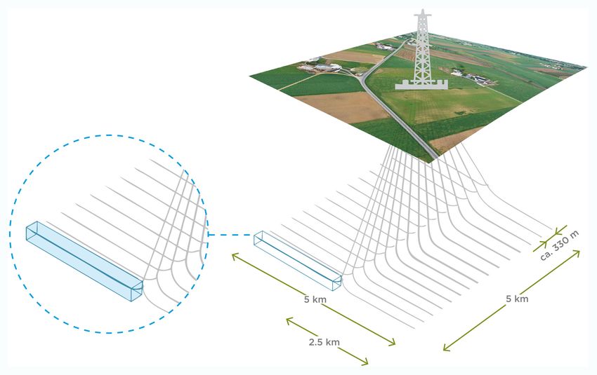
Art. 18, page 2 of 26 Cremonese et al: Emission scenarios of a potential shale gas industry in
Germany and the United Kingdom
CH4 emissions additionally have a negative effect on at extraction wells”,1 sources that can occur at any stage
public health due to the role of CH4 as a precursor of along the production chain and are therefore not neces-
ground-level ozone (O3; Garcia et al., 2005). Furthermore, sarily linked to fracking operations. Results from Omara
natural gas extraction and processing leads to emissions et al. (2016) show a correlation between the CH4 leakage
of air pollutants including volatile organic compounds rate and age of the wells rather than the nature of the
(VOCs), nitrous oxides (NOx), carbon monoxide (CO), and gas, proving that impacts related to other factors may, at
particulate matter (PM), which negatively affect human least occasionally, be greater than gas type. Data available
and environmental health (Dockery and Pope, 1994; for European gas plays is yet scarce. While US shale gas
Kampa and Castanas, 2008; Roy et al., 2014; Sweileh et al., leakages reported in Howarth (2014) can be higher than
2018). The dramatic increase in shale gas exploitation has 10%, data for conventional gas in countries like Germany
therefore raised concerns about the burden on the climate and the UK (NIR 2017) shows instead leakage rate below
and air quality. Accordingly, many studies have been 0.1%. This large emission discrepancy is widely applied to
conducted over the past years to examine the influence narratives on natural gas usage in the European context to
of shale (also called unconventional) and conventional gas oppose unconventional gas development. Nevertheless,
production on emissions, and on CH4 emissions in particu- Yacovitch et al. (2018) found high uncertainty in emission
lar. Especially in Europe, it is a shared belief among societal inventories from oil and gas wells in the Groningen Field
and political actors that emissions from conventional gas in the Netherlands, and the occurrence of an unidenti-
production are substantially lower than those from shale fied offshore super-emitter source. Moreover, preliminary
gas (DW, 2018; Energate, 2018; Zittel, 2015; Greenpeace, quantification of CH4 losses at North Sea offshore oil and
2015; Howarth, 2014). Although this was probably the gas platforms suggest much higher estimates than those
case at the onset of the shale gas boom when fracking reported by the UK national emission inventory, up to
operations were not properly regulated (e.g., open pits for 0.70% of the total gas produced (Riddick et al., 2019). All
storing flowback waters, improper well completion, etc.), of these studies performed in the US and emission dis-
rigid environmental standards are largely in place to date crepancies with European datasets do not conclusively
in the US. The latest scientific literature on this topic is prove large offsets between emissions from shale gas and
still ambivalent, and the preliminary – despite insuffi- conventional gas activities, and specifically do not explain
cient – data available seems to not support this large dis- much more conservative emissions for the latter. At the
crepancy: as reported in Zavala-Araiza et al. (2015), about same time, they neither prove the opposite. The emission
50% of emissions investigated in their study are attributed contribution of shale gas and conventional gas to total
to compressor stations and processing plants, and there- gas losses remains unclear to date, and further research
fore sources unrelated to the production technique. The is needed to reconcile emission budgets and rates among
remaining share is generated at production sites extract- these regions. This argument is further examined in the
ing both conventional and shale gas. Therefore, in the “Results and discussion” Section.
extreme and unrealistic case where hydraulic fracturing Notwithstanding that shale gas production has occurred
(i.e., the recovery technique employed during shale gas primarily in the US, global shale gas resources are consider-
extraction) were the only CH4 source at production sites, able, amounting to >200 tcm (trillion cubic meters) – or
the unconventional gas production chain would gener- rather, about one third of the world total technically recov-
ate about three-fourths of total emissions associated with erable natural gas reserves (EIA, 2013). Several European
natural gas production in the US. countries, including Germany and the United Kingdom
In support of this, hydraulic fracturing appears to not (UK), have expressed interest in recent years in utilizing
be responsible for larger emissions according to results by domestic shale gas assets as part of their national energy
Allen et al. (2013), despite the fact that emission budgets agenda. Although shale gas reserves in Germany and the
here might be underestimated due to the bottom-up data UK are substantially smaller than those found in, e.g., the
method applied (Brandt et al., 2014). Although Reduced US, production of shale gas has the potential to offset or
Emissions Completions (RECs) – a practice needed only at slow down the decline in conventional gas production
shale gas wells and able to cut emission by at least 90% that these countries are experiencing. This would avoid
during well completion (EPA, 2014a) – have been manda- increased dependency on foreign gas imports, as well as
tory in the US since January 2015, studies still continue avoid a potential increase in coal use for electricity gen-
to measure very high losses from overall gas recovery eration. However, opposition from the general public and
activities. One explanation might be that gas released environmental interest groups on account of potentially
during well completions, often alleged to be responsible harmful effects from shale gas fracking activities – for exam-
for augmented emissions at shale gas wells, have only a ple, surface and groundwater contamination (Osborn et al.,
minor contribution to total budgets. For example, Alvarez 2011; Jackson et al., 2013; Darrah et al., 2014; Drollette
et al. (2018) estimate an upstream leakage rate of 1.95% et al., 2015), increased frequency of earthquakes (Ellsworth,
from about 30% of all existing oil and gas wells in the US 2013), as well as increased emissions as discussed above
without reporting any evident discrepancy between these (Oltmans et al., 2014; Swarthout et al., 2015; Hildenbrand
two natural gas categories both present among the gas et al., 2016) – has led to moratoria and bans in various
plays analyzed. Yet, the EDF chief scientist and co-author regions and countries like in France and Germany. In the
of the study stated that “most [of the emissions detected] latter, the government recently placed a ban on unconven-
are tied to hatches and vents in natural gas storage tanks tional fracking at least until 2021 (Bundesregierung, 2017).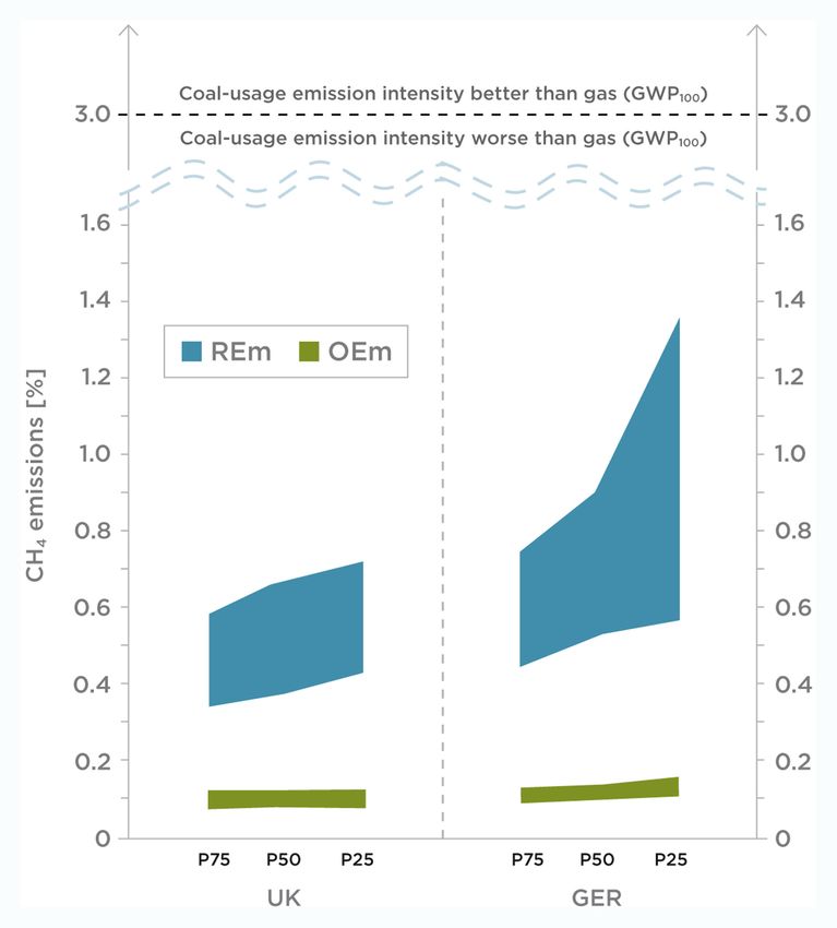
Cremonese et al: Emission scenarios of a potential shale gas industry in Art. 18, page 3 of 26
Germany and the United Kingdom
In the context of sustainability, a responsible energy parameter on the final results to guide the selection pro-
strategy with regard to shale gas production in Europe cess of such parameters.
requires sound scientific advice. Studies that explore what
the range of impacts that a potential European shale gas Shale characteristics and gas extraction
industry would entail, as well as opportunities to reduce Shale is a sedimentary type of rock that is generated by the
potentially harmful effects, are still missing although nec- compaction of deposits containing silt- and clay-size par-
essary to inform policy. Here we examine the impact of a ticles. While shale is characterized by extremely low per-
potential shale gas industry in Germany and the UK – two meability, it possesses a high porosity. It is in these pores
countries where political and social discussion on shale that the organic material and gas molecules are located,
gas has been intense over the last years – on GHG and as free gas or adsorbed on organic remains (Glorioso and
pollutant emissions, including CH4, CO2, VOCs, NOx, CO, Rattia, 2012). During the shale gas extraction process, a
PM10 and PM2.5 (PM ≤10 µm and ≤2.5 µm in diameter, vertical shaft is initially drilled. Then, when the vertical
respectively) through emission scenarios. First, we give drill path reaches the target shale formation – usually
an overview of shale characteristics and examine the between 1,000 and 4,000 m underground depending on
shale reservoirs considered in this work. Then, we discuss local geological features – its direction is shifted horizon-
how the drilling projections and emission scenarios are tally to follow the shale plane (Elsner and Hoelzer, 2016).
developed for Germany and the UK. Next, we describe Afterwards, water, sand, and chemicals are injected at
each of the scenarios that we designed, including the data high pressure to create fractures in the rock during the
that we incorporated and assumptions that we made. hydraulic fracturing or “fracking” process, increasing per-
Subsequently we present the results, i.e., the impact meability of the formation and thereby stimulating gas
of shale gas operations on emissions per each scenario. flow to the well (Gregory et al., 2011). Although most pub-
Finally, we analyze the impact on these two countries, put- lic attention tends to focus on the hydraulic fracturing,
ting the emissions into context with current inventories this recovery technique was performed experimentally in
to develop and transfer findings to policy-makers. The aim 1947 and has actually been in widespread use in Germany
of our scenarios is to understand what a shale gas indus- since the 1960s (LBEG, 2010; Wilson and Schwank, 2013).
try in Europe may look like, to show how regulation and In fact, horizontal drilling is the more recent technol-
compliance (along with uncertainty ranges) may impact ogy and game changer that has made commercial shale
emissions, and to present opportunities for air quality and gas production possible. Horizontal wells – which can
emission mitigation. extend over several kilometers – maximize contact with
Other potential consequences of shale gas production, the shale payzone which is typically spread out in narrow,
such as surface and water contamination, seismic activity, horizontal bands, whereas vertical wells can only provide a
and an offsetting of emissions from coal in electricity gen- small, insufficient portion of contact (Pearson et al., 2012;
eration due to availability of natural gas, are important but ACATEC, 2016). Furthermore, directional drilling is used
outside the scope of this study and are not be considered to reach targets beneath adjacent lands, intersect frac-
here. A follow-up study will explore the potential impact tures, and drill multiple wells from the same vertical bore-
of shale gas emissions on local and regional air quality in hole (Elsner and Hoelzer, 2016), thereby maximizing the
Europe through atmospheric chemistry modelling. shale gas yield while reducing the surface environmental
footprint.
Methodology
In this study we investigate realistic shale gas industrial Shale reservoirs considered in this study
developments in Germany and the UK, and quantify their The shale gas reservoirs taken into account in the present
associated GHG and air pollutant emissions. In order to do study are based on recent studies which aimed to quan-
this, we first develop drilling projections in which we esti- tify the relevance of shale gas as a national energy asset
mate the total number of “wells under construction” and by both the German and British governments. In its 2016
“producing wells” required to achieve and maintain steady- report, the Federal Institute for Geosciences and Natural
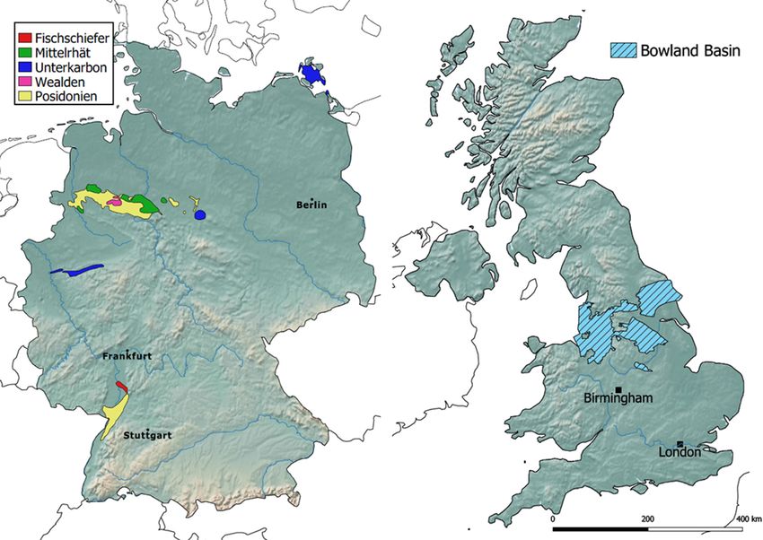
state gas production in the two countries of reference, Resources (BGR, 2016) found five shale basins in Germany to
based on varying degrees of well productivity. After that, be promising for natural gas production: the Fischschiefer,
we quantify emissions associated with upstream produc- Wealden, Posidonien, Mittetrhät, and Unterkarbon units.
tion through a bottom-up approach in different scenarios These basins are scattered across several federal states,
covering a series of well productivity and technology/per- covering a total area of more than 8,000 km2, and are
formance cases. The results presented here are plausible buried between 500 and 5,000 m underground. The tech-
under specific geological and technological/performance nically Recoverable Resource (TRR) for these reservoirs
conditions selected in this study and consistent with the ranges between 650 and 1,380 bcm (billion cubic meters),
existing scientific literature. Results and their interpreta- averaging at 940 bcm. By comparison, the UK’s geologi-
tion reported in the discussion section, as well as their cal landscape is characterized primarily by one major
scientific relevance, have to be therefore evaluated taking shale basin, the B owland-Hodder Carboniferous Unit.
such constraints into account. Additionally, a sensitivity This basin spans an area of 14,000 km2 underneath the
analysis of the emission scenarios is performed and is pro- regions of Yorkshire, North West, East and West M idlands
vided in the SM, Text S1, Section S3. The purpose of this is and reaches a maximum depth of 4,750 m below ground.
to examine the contribution and influence of each varying According to the B ritish G
eological S urvey’s (BGS) 2013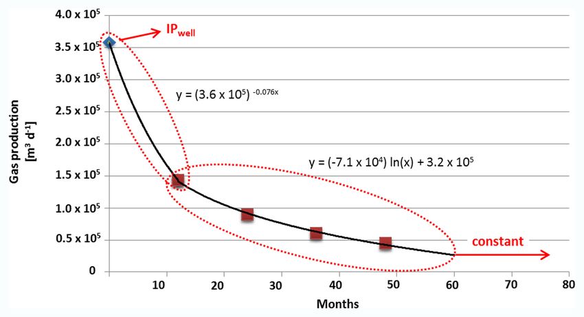
Art. 18, page 4 of 26 Cremonese et al: Emission scenarios of a potential shale gas industry in
Germany and the United Kingdom
report, the total gas-in-place (GIP) buried in this forma- uncertainty range described by three cases of productiv-
tion is estimated at 37.6 tcm (trillion cubic meter), while ity: 25th, 50th, and 75th percentile of exceedance, which
the TRR is still unknown. Pilot exploration projects by we refer to as P25, P50 and P75. Following the approach
Cuadrilla are planned and started again in late 2018, after adopted by the BGR, the TRR of the Bowland Basin was
a long break following the Blackpool Earthquake in 2011. calculated as 10% of the total GIP range estimated by the
The shale reservoir locations in G ermany and the UK are BGS. In this study, P25 and P75 signify low- and high-basin
shown in Figure 1. These basins are selected as the gas productivities respectively, while P50 describes the “most
reservoirs to be exploited in our drilling projections. likely” case. Due to the lack of data and to reduce com-
plexity, we assume that each of the six basins contains a
Drilling projections homogeneous gas density across their geographical exten-
Three different projections of shale gas well populations sion (i.e., no hot spots are considered). The gas “density” is
are developed for Germany and the UK in this work, calculated for each basin and productivity case. Data are
referred to henceforth as drilling projections. The drill- reported in SM Text S1, Table S1. TRR results are showed
ing projections ultimately provide information on the in Table 1.
number of wells under construction and producing wells, Step 2: Well Estimated Ultimate Recovery (EURwell). In
information that is necessary to quantify emissions from order to assess the productivity of the wells (the total gas
shale gas production in the emission scenarios. In the next output from a single well during its lifetime) for each pro-
paragraphs we describe the four main steps involved in ductivity case (P25, P50 and P75) and for each basin, we
building the drilling projections and the critical assump- have to define the portion of reservoir that is exploited
tions made. by a single horizontal well. To do this, we assume that
Step 1: Basin productivity. We first define the extension each well pad exploited an area of 25 km2, from which 30
of the shale gas prospective basins described in the pre- horizontal wells are drilled (Figure 2; Pearson et al., 2012;
vious section. Subsequently we considered the Technical Acatech, 2016). Based on the gas densities estimated in
Recoverable Resources (TRR), defined by national authori- step 1, we are able to define the EURwell that character-
ties as the volume of gas that can be produced with cur- izes each population of wells. More information on the
rently available technology and practices. The estimated assumptions on which we base this well geometry is avail-
TRR of the shale gas basins is typically provided in an able in the SM, Text S1, Section S1.1.
Figure 1: Shale gas basin areas for Germany (left) and the UK (right). Figures include legends with the basin
names and their designated color on the map. DOI: https://doi.org/10.1525/elementa.359.f1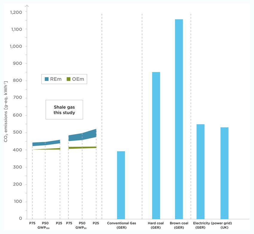
Cremonese et al: Emission scenarios of a potential shale gas industry in                                    Art. 18, page 5 of 26
Germany and the United Kingdom

Table 1: Shale gas basin characteristics and well data at steady-state production. Area and TRR of all shale gas
  basins for both Germany and the UK. The number of years required to achieve the desired volume of gas for each
  productivity case under each basin productivity and emission scenario is also indicated. The ranges of wells under
  construction and producing wells represent the variance between the upper and lower boundary for each case. DOI:
  https://doi.org/10.1525/elementa.359.t1

         Country     Productivity      Area     TRR  Years to               Wells at the steady-state production
                     Case             [Km2]    [bcm] maturity         Optimistic Emissions       Realistic Emissions
                                                                            (OEm)                       (REm)
                                                                    Under con-     Producing   Under con-   Producing
                                                                     struction                  struction
         Germany P25                              550           8            162 1,927–1,937     164–166 1,952–1,979
                     P50               8,341      801           3            143     867–872     144–146      879–891
                     P75                        1,182           2          97–98     522–525      99–100      529–536
         UK          P25                        2,866           4      201–202 1,407–1,414       204–206 1,426–1,445
                     P50             13,736     3,760           2      160–161       856–860     162–164      867–879
                     P75                        5,447           1            110     479–482     111–113      486–492

Figure 2: 3D underground view of well geometry. We assume that a total of thirty underground horizontal wells are
  drilled on a single well pad, which covers an area of 25 km2, as shown in the figure. DOI: https://doi.org/10.1525/
  elementa.359.f2

  Step 3: Well productivity curve. Shale gas wells present          EURwell for each basin is defined, we estimate the Initial
a steep production curve: After about one or two years of           Production (IPwell) of each population of wells through
sustained production, their yield decreases substantially           the Rie factor. This coefficient is based on the correla-
according to the geological characteristics of the shale            tion between EURwell and IPwell observed in the Barnett
reservoir (Patzek et al., 2013). This pattern is generally          and the Eagle Ford plays, two US basins that show pet-
described by a curve declining asymptotically toward zero           rological similarities with the German Unterkarbon and
production (i.e., exhausted well). Here, we describe how            the Posidonia shales (BGR, 2016). To reduce complexity,
the declining curve of the wells is determined. Once the            their IPs and production declining rates are averaged and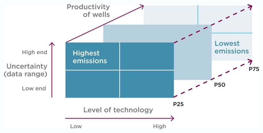
Art. 18, page 6 of 26                                    Cremonese et al: Emission scenarios of a potential shale gas industry in
                                                                                              Germany and the United Kingdom

applied to all the German and UK basins investigated           selected from the projections Germany P50 and UK P50.
here. Rie is defined as:                                       Once the gas flowing from producing wells – the popula-
                                                               tion of which grows annually due to continuous drilling
                                 IPwell                        activity –reaches these volumes, we calculate the number
                        Rie =
                                EURwell                        of annual new wells required to maintain this production
                                                               level for both Germany and the UK. In fact, this param-
The resulting production decline curve is best described       eter varies over time since it depends on the number of
with an exponential trend in the first year (Patzek et al.,    existing producing wells, their age and declining rate, and
2013), and logarithmic trend for the following four years      the total gas output. Therefore, we considered the aver-
as shown in Figure 3.                                          age over the following three years. This value, specific to
   For each basin, the same declining pattern describes the    each country and productivity case, is defined as wells
production variation over time, specific to each productiv-    under construction. The drilling projections also provide
ity case. After the fifth year, we assume that gas produc-     details of the number of active wells (i.e., producing wells)
tion remains constant because of our limited knowledge         at steady state production in each country and produc-
of long-term trends.                                           tivity case. The output data from each drilling projection,
   Step 4: Estimating the population of wells under con-       namely wells under construction and producing wells, are
struction and producing wells. These values are based on       used as input in the emission scenarios. The results are
regional settings and comparisons with the development         shown in Table 1 and SM Text 1, Figure S1.
rates of US shale plays (Hughes, 2013). We estimated that
200 new wells are drilled each year in Germany and 280         Emission scenarios
in the UK. These estimates represent the final number          The emission scenarios are generated by compiling and
of wells drilled, taking into account a failure rate of 20%    aggregating emissions estimated at each stage of the sup-
(i.e., unsuccessful wells). Moreover, the wells are numeri-    ply chain (i.e., from well preparation to gas processing) at
cally distributed among the different German basins pro-       industrial maturity. By feeding the system with the out-
portionally to the basins’ extension. The drilling rates are   puts parameters of the drilling projections (wells under
kept constant in the two countries until a gas output of       construction and producing wells) for both Germany and
11.58 bcm for the former and 36.62 bcm for the latter          the UK, we quantify emissions for each country under
is achieved at industrial maturity. These two values are       diverse basin productivities and production settings (i.e.,
selected from among all the gas output results obtained        performance in recovery practices and different technolo-
by the three drilling projections developed for each coun-     gies). The category wells under construction is associated
try, since they best fit with historical data and realistic    with the stages well pad development, trucks and water
national goals of the region under observation (see dis-       pipelines, drilling, fracking and well completion, while the
cussion in SM Text S1, sections S1). Specifically, they are    producing wells is associated with the stages gas produc-

Figure 3: Example of well declining production curve in our scenarios – Unterkarbon (Germany), P50. The
  declining curve, extrapolated from the Eagle Ford and Barnett shale plays in the US and tailored to the EUR and IP of
  our case study reservoirs, follow an exponential trend in the first year, and a logarithmic trend in the following 4 years
  (see equations in the figure). From the 5th year onwards, we assume that production remains constant. DOI: https://
  doi.org/10.1525/elementa.359.f3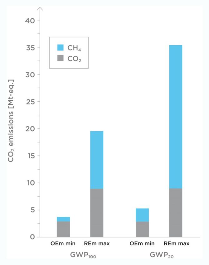
Cremonese et al: Emission scenarios of a potential shale gas industry in                                             Art. 18, page 7 of 26
Germany and the United Kingdom

tion, wellhead compressor exhausts, liquids unloading,                   challenging case where emission reduction technologies
gas gathering and processing. Emissions are calculated                   (e.g., electric motors instead of diesel-engines) and all best
by combining activity data and emission factors for each                 practices and monitoring services are in place and fully
stage of shale gas production, depending on the technol-                 employed across the supply chain (e.g., no damages of any
ogy and uncertainties associated with each specific sce-                 component, no malpractice and abatement of unwanted
nario. Activity data represent the magnitude of activity                 gas losses). This case is defined as the most optimistic case
that results in emissions, while emission factors represent              and represents the lowest technical emission boundary
the gas released per unit of a given activity, and are typi-             achievable according to the technologies and practices
cally provided as a range. All input parameters are based                considered in this study and described in detail in Table 3
on official reports, expert support and peer-reviewed pub-               and SM Text S1, Section S2. REm and OEm illustrate the
lications, most of which focused on US shale gas plays                   degree to which these two different cases can affect emis-
since shale gas production has hitherto mostly occurred                  sions of the suite of pollutants and GHGs under study,
there. Additionally, the input parameters include our own                and they provide a clear indication on possible mitigation
critical assessments of how to best apply the data to the                potential of different options. Obsolete technologies or
European cases proposed in this study (described in fur-                 practices that we expect not to be permitted in Europe
ther detail in SM, Text S1 Section S2). Where available, we              are not considered in any scenario: e.g., open-air pits,
opted for large sample-size surveys, with a preference for               improper well completions (SM Text S1, Section S2.6), low
results by accredited research groups such as the Environ-               number of wells per pad (SM Text S1, Section S1.1), insuffi-
mental Defense Fund (EDF, 2019). A list of the parameters                cient environmental standards during the liquids unload-
and variables that determine emissions as well as the ref-               ing practice (SM Text S1, Section S2.9), lack of recycling of
erence literature is reproduced in Table 2. To realistically             fracking/drilling waters (SM Text S1, Section S2.3), and so
assess VOC emissions as a by-product of natural gas pro-                 forth. These scenarios are informative for evaluating best
duction, we also varied the VOC component of natural gas                 recovery practices to outline new environmental regula-
to examine the impact of both wet and dry gas on total                   tions for drilling and producing. The main technologies
VOC emissions according to gas composition reported by                   and operations that differentiate REm and OEm are listed
Faramawy et al. (2016).                                                  in Table 3, while a complete description is available in SM
   Our emission scenarios are divided into two overarching               Text S1, Section S2.
categories based on varying technologies/performances at                    Due to data uncertainty and unpredictable intrinsic vari-
each stage of gas production, namely “realistic” and “opti-              ables (e.g., number of fracking stages, uncertainty in values
mistic” emission scenarios (abbreviated as REm and OEm).                 reported by the source agency, etc.), a range of emissions
REm refers to practices and standard technologies used                   are developed for REm and OEm. Therefore, both scenar-
for gas exploitation and management which generate                       ios can be further broken down into “upper” (U) or “lower”
relatively high emissions (i.e., business as usual), and are             (L) categories that define the ranges of uncertainty. “U”
still largely used in the US and Europe. This case is consid-            results define the high end of the emission range, while
ered the realistic case that we expect for the two European              “L” results define the low end. Altogether, this produces
countries examined. On the other hand, OEm refers to the                 four scenarios (from the lowest to the highest emissions):

Table 2: List of parameters and variables defining emission variations between REm and OEm. Sources of
  data are also provided. Note that EF stands for emission factor. DOI: https://doi.org/10.1525/elementa.359.t2

 Activity                 Parameters/variables defining emission scenarios                    Source of reference
 Well pad development Length of operations, EF diesel motors                                  NYSDEC (2015); Helms et al. (2010);
                                                                                              European Emission Standards.2
 Truck Traffic            EF of truck motors, re-suspended particles, road type; materi- IVT (2015), NYSDEC (2015); EMEP/EEA
                          als, water and chemicals supply, waters recycle rate and          (2016); Denier Van Der Gon et al. (2018);
                          “piped” vs. “trucked” rate, average well length, fracking stages. Statista; CottonInfo (2015).
 Drilling                 Diesel generators vs. electricity; total wells length.              Pring et al. (2015); Helms et al. (2010).
 Fracking operations      # fracking stages, length of operations, diesel engines EFs.        Roy et al. (2014); Helms et al. (2010).
 Well completion          Emissions at operations.                                            Allen et al. (2013).
 Production sites         Diesel vs. electric compressors, gas emissions at facility.         Omara et al. (2016); ICF (2014).
 Wellhead compressors Diesel/electric compressor.                                             NYSDEC (2015); Helms et al. (2010).
 Liquids unloading        Automatic vs. manual plunger lifts, operations per well             Allen et al. (2015)
 Gathering facilities     Gas loss at facility, number of wells connected to the facility,    Mitchell et al. (2015); Marchese et al.
 and pipelines            gas loss from pipelines                                             (2015); Helms et al. (2010);
 Processing               Gas loss at facility, gas turbine efficiency                        Mitchell et al. (2015); EPA (2000);
                                                                                              Müller-Syring et al. (2016)
Art. 18, page 8 of 26 Cremonese et al: Emission scenarios of a potential shale gas industry in
Germany and the United Kingdom
OEm-L, OEm-U, REm-L and REm-U. To visualize the tivities (P25, P50 and P75), for both wet and dry gas, for
breadth of our scenarios, we have represented them as a different GHGs and air pollutants, and for both countries
three-dimensional cube in Figure 4. under study (Germany and the UK). Both CH4 and CO2 emis-
sions from our shale gas scenarios display significant differ-
Results and discussion ences in REm and OEm in both countries. In the following
GHG emissions in shale gas scenarios paragraphs we focus on wet gas scenarios, while we refer to
In this section we examine annual emission results from dry gas scenarios only occasionally: emission trends from
all the scenarios developed in this study and extensively dry scenarios closely resemble those from wet scenarios,
described in the methodology section and SM Text 1 with the exception that VOCs make up a very small com-
sections S1 and S2. We discuss results under the two tech- ponent of the gas composition. Total CH4 released in REm
nological/performance settings employed during shale gas ranges between 104 and 175 Kt in the UK, and between
development (REm and OEm), under differing well produc- 46.4 and 78.5 Kt in Germany in the P50 cases (Figure 5).
Table 3: List of major differences in the technologies applied to REm and OEm scenarios. DOI: https://doi.
org/10.1525/elementa.359.t3
Activity Data REm OEm
Motor type Diesel-engines are used during all stages. Emission Electrified motors applied at some of the production
factors for non-road diesel machineries refer to the stages at gathering. Emission factors for the national
inventory from the German Environmental Agency electric grid are available from the German Environmen-
(Helms, 2010). tal Agency (UBA, 2017) and are applied to Germany and
the UK.
Fracking waters Fracking waters are transported to the well site via All fracking waters are piped to the well site, with high
management trucks, with low recycling rates (50%). Emission recycling rates (90%). Emission factors for trucks (Euro6)
factors for trucks (Euro3/6) are available from the are available from the IVT database (IVT, 2015).
IVT database (IVT, 2015).
Turbines The volume of gas combusted to fulfil energy Volume of gas combusted to fulfil the energy require-
(processing) requirements during processing is calculated accord- ment during processing is calculated according to the
ing to the efficiency and performance of a simple efficiency and performance of a combined cycle, water
cycle, uncontrolled turbines. steam-injection turbines.
Emission factors Emission factors for all engines categories are Emission factors for all engines categories follow recent,
conservative. strict national, legally-binding emission standards.
Well structures Well ramifications (horizontal wells) at the bottom Well ramifications (horizontal wells) at the bottom of
of each vertical well: 3. each vertical well: 10.
Figure 4: 3D cube representation of shale gas emission scenarios. On the x-axis is the level of technology which is
based on the level of regulation; the y-axis represents the uncertainty range in the data, and the z-axis represents the
productivity of the wells from the three drilling projections (i.e., P25, P50 and P75). DOI: https://doi.org/10.1525/
elementa.359.f4Cremonese et al: Emission scenarios of a potential shale gas industry in Art. 18, page 9 of 26 Germany and the United Kingdom Figure 5: CH4 and CO2 annual emissions from our study for Germany and the UK. The dot lines in red rep- resent the emission volumes as reported by the UNFCCC for the year reported. DOI: https://doi.org/10.1525/ elementa.359.f5 On the other hand, under the P25 well productivity case results: OEm-L P75 and REm-U P25 for the lower and maximum CH4 emissions reach 196 and 119 Kt for the UK upper bounds, respectively. CH4 released during well and Germany respectively, while in P75 values are not sig- preparation stages (i.e., excavators, well pad configura- nificantly lowered beyond the P50 case. Low well produc- tion and construction) are trivial when compared with tivity therefore translates into significantly enhanced CH4 total emissions generated by the whole chain. From well emissions, especially in Germany. The wells’ steep produc- construction up until hydraulic fracturing (i.e., drilling tion curve characterizing shale reservoirs overall, along activities, water, sand and equipment moved by trucks, with lower volumes of recoverable gas in this specific case fracking and well completion) a maximum of 0.5 Kt CH4 justify the higher drilling rate necessary to maintain pro- for both countries are lost over the entire year, mostly con- duction constant. The resulting larger population of active centrated at well completion. Strict emission mitigation wells in both categories producing wells and wells under measures deployed in the OEm can facilitate reductions construction are ultimately responsible for augmented by a maximum of circa 50%. CH4 leaked or vented by com- emissions. On the contrary, CH4 losses generated by OEm pressors, valves, joints and gaskets, represents an impor- are significantly lower and within a narrow range among tant contributor under REm (19 to 33 Kt in Germany, 62 the different productivity projections. Here the ranges are to 108 Kt in the UK), while consolidation of wells onto from 21.5 to 31.3 Kt for the UK, while from 7.4 to 11.0 centralized well pads (more horizontal wells per vertical Kt in Germany. CO2 emissions in REm range from 3.7 to well; see also Robertson et al., 2018) combined with sub- 4.9 Mt in the UK and 1.8 to 2.3 Mt in Germany under the stitution of diesel engines with electrically-powered ones P50 scenario case. While low well productivity in REm as foreseen in OEm limits losses at production site to ca. increases emissions in the UK to a maximum of 5.5 Mt, 3 and 11 Kt in Germany and the UK, respectively. Since in Germany the increase is proportionally higher reaching uncombusted gas and wet seals in diesel and natural gas- almost 3.4 Mt. CO2 emissions in OEm range between 2.2 powered compressors are the main sources of fugitive and 2.7 Mt in the UK (P50), and between 0.9 and 1.2 Mt in CH4, replacement with electric compressors can eliminate Germany (P50). The distribution of GHG emissions across emissions (Kirchgessner et al., 1997; Marchese et al. 2015 the production stages and their variability under different Supporting Information; Mitchell et al., 2015 Supporting technological/performance cases and for each country are Information). Similar reductions (of ca. 95%) can be shown in Figure 6. achieved by implementation of dry-seal compressors with In the following discussion we focus on results from flaring systems (EPA, 2014b). the P50 scenarios, with reference to the other productiv- Wellhead compressors and liquids unloading (both ity cases when significant emission variations warrants with manual or automatic plunger lifts) have a very lim- further analysis. Nevertheless, the emission boundaries ited impact on total figures. The former are employed to for our scenarios are reported in all diagrams displayed increase the gas yield from low-pressure reservoirs, while in Figure 6 to represent the range of variability in our the latter is a practice necessary to unclog the wells when
Art. 18, page 10 of 26                             Cremonese et al: Emission scenarios of a potential shale gas industry in
                                                                                        Germany and the United Kingdom

Figure 6: Annual cumulative emissions along the shale gas production chain. Results for CH4, CO2, NOx and PM10
  for Germany (GER, left) and the UK (right). REm and OEm are shown for the P50 case, while REm-U P25 and OEm-L
  P75 are also reported to show the emission boundaries. DOI: https://doi.org/10.1525/elementa.359.f6
Cremonese et al: Emission scenarios of a potential shale gas industry in Art. 18, page 11 of 26 Germany and the United Kingdom large amount of liquids accumulate in the borehole. At at this stage – mainly driven by turbine efficiencies – can the gathering stage, regardless of how compressors are potentially reduce emissions between 30 and 40%. Well- operated, CH4 losses (which include both gathering pipe- head compressors and fracking are next in order of impor- lines and gathering facilities, SM Text S1, Section S2.10) tance although they only account for 2 to 15% of total CO2 represent 35–48% of total emissions generated by the emissions in almost all scenarios for both countries. scenarios in Germany, and 24–41% in the UK. Here again, mitigation measures applied in OEm appear to be effec- GHG emissions national contexts tive, decreasing CH4 emissions by as much as 87% to Here we compare our results of GHG emissions from shale 88% in Germany and 83% to 87% in the UK (low and gas with emission inventories supplied to the United high emissions boundaries, respectively). Because of the Nation Framework Convention of Climate Change (UNF- high emission factor associated with each gathering facil- CCC) for the energy industrial system (i.e., power and heat ity (Marchese et al., 2015; Mitchell et al., 2015) and also production, petroleum refining and manufacture of solid enforced in our emission exercise, reducing the number fuels). For this scope, we select the year 2012 for Germany of gathering facilities collecting the gas from the produc- and 2015 for the UK as reported in the National Inventory tion areas appear to contribute significantly to reduced Report (NIR) year 2017 submission, since the conventional gas losses. The number of these facilities is strictly linked gas domestically produced in these years is similar to the to the geographical location of the producing wells, and ones assumed in the scenarios: 10.7 bcm for Germany to the technical feasibility and economic convenience to and 34.4 bcm for the UK.3 Focusing on the UK, CH4 and connect them to a single (large) or more (smaller) gather- CO2 generated by the well-preparation stage till process- ing plants. We assume one gathering facility for every 30 ing (namely, upstream) of the current natural gas indus- wells in REm, and one for every 80 wells in OEm (SM Text try only contributed 7.0% (CH4) and 0.4% (CO2) of total S1, Section S2.10.1). In the latter, emissions are mainly emissions from the industrial energy sector for the UK. For controlled by substitution of diesel to electric engines. the former, shares from the OEm P50 scenarios of total At gathering facilities, emission factor standards for die- gas released from the energy sector are similar in magni- sel engines have negligible effects, while gas losses com- tude, while emissions under REm P50 settings achieve 30 bined with the number of gathering facilities dominate (REm-L) to 65% (REm-U) of reported current datasets for this gas production stage contributing up to circa 90% the UK (up until 70% under P25). All results are reported in Germany and 70% in the UK of total CH4 emissions. in Table 4. Most of the offshore gas produced in the UK On the other hand, emissions from gathering facilities in requires processing (UNFCCC, NIR for the UK, year 2017 OEm are significantly lower (circa 10% of CH4 emitted in submission) due to its variable but still notable content of REm for Germany and between 20 and 30% for the UK), impurities like CO2, nitrogen, ethane, and so on (Cowper where gathering pipelines contribute to more than 65% et al., 2013). The conservative emission estimates from the in Germany and 87% in the UK of total CH4 emissions in current UNFCCC Report may be justified assuming that the gathering sector. It is worth noting that in REm-U P25 best practices for CH4 capture are all in place and prop- scenarios CH4 emissions from gathering are particularly erly performed, keeping them down to a level comparable higher than the ones in P50 (50% higher in Germany and with the lowest depicted by our scenarios. On the other 35% in the UK), highlighting the impact that low well pro- hand, the CO2 relative contribution to emission from the ductivity (especially in Germany) has on gathering sector energy industry raises from 0.4 to 1.6% when comparing emissions. The prominent role of CH4 emitted at gather- results from the UNFCCC Report with OEm or until 3.5% ing facilities and production sites finds confirmation in with REm. Therefore, even under our most conservative the literature (Zavala-Araiza et al., 2015; Balcombe et al., scenario contemplating the highest combustion turbine 2016; Littlefield et al., 2017). The gas processing stage, as efficiency and the lowest combustion rate of gas dur- characterized in our study (between 2.8% and 5.6% of ing high-emitting processing activities, CO2 emissions gas burned for power production and turbines efficiency reported by the UNFCCC are about one fourth of these. between 30% and 60%; SM Text S1, Section S2.11.2), In Germany, CH4 emitted from the natural gas upstream comes only third in terms of CH4 emissions contribution system contribute about 0.6% of the total emitted by after the gathering and production stages in REm, while the national energy system, while CO2 only 0.4%. This is second in OEm. This is because best practices aiming to mostly due to the high consumption of solid fuels in the reduce the overall losses from processing plants are able country that brings coal (and lignite in particular) far to to drive emissions down by about 50% overall. Other the top of the list of emitters: CO2 released from natural factors such as turbine efficiencies, combusted gas for gas combustion are similar for the two countries, while energy needs and emission factors are, for this pollutant, those generated in Germany by solid fuels are four times irrelevant for both countries and scenarios. Gathering and more than in the UK (UNFCCC, NIR submission 2017 for processing of shale gas dominate total CO2 emissions in both countries). CH4 emissions produced by our scenar- all scenarios, spanning from 55% in OEm to 70% in REm. ios raises contributions to a range of 1.6 to 2.4% of total Mitigation measures such as electrification of all compres- energy from the industrial system emissions in OEm, and sors and pumps applied in OEm at gathering facilities up to 10.3%–17.4% in REm. This means that the natural are particularly efficient to cut gas losses at this stage by gas sector is an important contributor requiring appropri- ca. 75% in both countries. Similarly, the amount of gas ate attention by regulators when prescribing technolo- burned to produce electricity and fulfil the energy needs gies, monitoring and verification systems, in G ermany
Art. 18, page 12 of 26 Cremonese et al: Emission scenarios of a potential shale gas industry in
Germany and the United Kingdom
Table 4: Annual CH4 and CO2 emissions generated by our shale gas industry for Germany (GER) and the UK.
Results are compared with emissions of the current upstream natural gas chain and the energy (heat and power)
sector as described by the UNFCCC. Please note that the term “fugitive” in the UNFCCC reference relates to all m
ethane
emissions associated to that specific stage. DOI: https://doi.org/10.1525/elementa.359.t4
Species Fuel combus- Fugitive Emissions OEm P50 results as share REm P50 results as share
tion emissions – emissions gas upstream of current emissions of current emissions
Energy industry fossil fuels (UNFCCC, (Range boundaries). In Kt. (Range boundaries). In Kt.
(UNFCCC, (UNFCCC, 2017) and
2017). In Kt. 2017). In Kt. share
GER CH4 89.9 366 2.7 (0.6%) 7.4 (1.6%) to 11.0 (2.4%) 46.4 (10.3%) to 78.5 (17.4%)
GER CO2 359,000 2960 1590 (0.4%) 924 (0.3%) to 1213.0 (0.3%) 1830 (0.5%) to 2330 (0.6%)
UK CH4 12.1 258 19.5 (7.0%) 21.5 (7.9%) to 31.3 (11.6%) 104 (30%) to 175 (65%)
UK CO2 133,000 4560 514 (0.4%) 2,190 (1.6%) to 2,750 (2.0%) 3,726 (2.7%) to 4,880 (3.5%)
as in the UK. On the other hand, CO2 generated by the studies produced by the Environmental Defense Fund ini-
German shale gas industry maintain emissions from 0.2 tiative and others (Sauter et al., 2013; Elsner et al., 2015;
to 0.6% (Table 4), to a maximum of 0.9% in the REm P25. Omara et al., 2016; Atherton et al., 2017). Based on the
Of total gas produced in Germany, 40% has high sul- latest evidence, gas capture solutions, “detection and
fur content (sour gas) that has to be discarded by specific repair” services, as well as monitoring and early detection
treatments before the gas can access transmission lines. of super-emitters are the most likely key measures when
In the UNFCCC NIR submissions 2017 for Germany, CO2 it comes to effectively mitigate emissions for both gas
and CH4 emission factors for removing sulfur are 336 and sources (EPA, 2014a; Westaway et al., 2015; Ravikumar and
0.11 kg per 1,000 m3 of treated gas respectively. The only Brandt, 2017; Zavala-Araiza et al., 2017; Konschnik and
CO2 and CH4 emissions associated with the processing Jordaan, 2018). Unfortunately, surveys that investigate
stages of gas reported are those related to the treatment European CH4 losses in a transparent and systematic way
of sour gas, while no other emissions attributed to pre- (e.g., peer-reviewed articles published by independent
treatments occurring at pumping stations (such as water, research bodies) do not exist or are not publicly available,
hydrocarbons and solid removals), are listed. We therefore raising doubts over the accuracy and objectivity of emis-
assume that in the current gas extraction industry, no CO2 sion estimates provided to the UNFCCC (EC, 2015; Larsen
or CH4 emissions are associated with, or rather expected et al., 2015; Cremonese and Gusev, 2016; Riddick et al.,
from, pre-treatments, an aspect for which we believe 2019). To facilitate identifying CH4 emissions specifically
deserves further investigation into the reliability of such from a future European shale gas industry, for instance
an assumption. Visschedijk et al. (2018) propose an atmospheric ethane
Despite the relevance of discussing our results in monitoring system. Because of these research gaps, we
the context of national inventories, it is challenging to find it hard to justify such a large discrepancy by citing
explain the inconsistency in the results for REm (and technological, regulatory or geological factors alone. The
from the US) with the emissions reported for Germany results shown in OEm are instead much more similar to
and the UK under the UNFCCC. A study of CH4 emitted European national inventories. Namely, the leakage rate
from the Groningen field in the Netherlands by Yacovitch as calculated by data from the UNFCCC NIRs is as low as
et al. (2018) also struggled to provide an explanation for 0.02% for Germany and 0.08% for the UK. Based on our
the large emission discrepancy between their campaign discussion and results, these estimates may be justified by
observations and national inventories. The authors of the systematic employment and application of best technolo-
same study believe that major differences between North gies/performances across each stage of the preparation
American and European estimates cannot be ascribed to and supply gas chain – a rather unlikely circumstance.
the large-scale adoption of hydraulic fracturing in the for- Given the fact that there is no transparent information
mer. Riddick et al. (2019) also report high and unreported available on the quality of these estimates, we speculate
CH4 losses from oil and gas wells in the North Sea, criti- that they could be based on very optimistic assumptions
cizing bottom-up methods and self-reporting by opera- (i.e., as the ones we apply in OEm) instead of systematic
tors as an improper practice. Our findings displayed in and integrated monitoring campaigns (see also discussion
Figure 6 also show that emissions generated at stages in Riddick et al., 2019).
that are specific to shale gas activities (i.e., well comple-
tion and fracking) have only a minor effect on total CH4 CO2 and CH4 contribution to total GHG emissions
losses when RECs are in place (SM Text 1 Section S2.5 and The warming-related contribution of CH4 – a much more
S2.6). Most critical CH4 and air pollutant sources across potent GHG than CO2 – is subject to the time frame of
the gas chain have been attributed to above-ground mal- observation. This effect is controlled by the oxidation
practices, failures or malfunctions unrelated to the gas of CH4 to CO2 (t1/2 ~ 12years; Myhre et al., 2013), so that
nature (i.e., conventional or shale gas), as reported by the its warming component in the atmosphere decreasesCremonese et al: Emission scenarios of a potential shale gas industry in Art. 18, page 13 of 26
Germany and the United Kingdom
with time. Two Global Warming Potentials (GWPs) are all scenarios (with a peak of 76%), while between 22 and
commonly used in the scientific community: the GWP100 55% assuming a GWP100. REm and OEm differ based on the
and GWP20, with the numbers referring to the warming performance of practices and implementation of diverse
implications over those periods of time, respectively 20- technologies to monitor and control CH4 losses on the one
and 100-years (IPCC, 2014). While these two parameters hand, and to increase efficiency of engines and compres-
are complementary and can offer a comprehensive over- sors so as to curb emissions of CO2 on the other hand. It is
view on the implications of this pollutant in the short- evident here that, although CO2 emissions can be cut up
and long-term, one indicator may be preferred instead to ca. 60% (difference between the REm and OEm CO2-
of the other according to the scope of a specific research bars in both GWP scenarios), CH4 reduction measures are
exercise (Ocko et al., 2017; Balcombe et al., 2018). Total by far more effective and can technically reduce CO2-eq.
aggregated GHG emissions (CO2-eq) from the shale gas CH4 emissions by 92%. Full compliance with the overall
upstream sector and covering all well productivity cases settings applied in OEm has notable climate benefits on
are shown in Figure 7, applying both 20- and 100-year reducing aggregated CO2-eq. volumes by a factor of maxi-
periods. mum 5 in the GWP100 case, and by a factor of maximum 7
On a mass-to-mass basis, CO2 emissions are significantly in the GWP20 case.
higher than CH4 because of the large amount of natural
gas combusted to CO2 at processing plants to fulfil the Methane leakage rates in the international context
power demand (SM Text S1, Section S2.11.2). Our aggre- Figure 8 shows the CH4 losses already reported in Figure 5,
gated upstream shale gas industry displays much higher in relation to overall CH4 production and expressed in per-
variability between REm and OEm, than between analysis centage for all productivity and technological scenarios.
under GWP20 and GWP100. Results in OEm are comparable Accordingly, CH4 emissions from associated activities are
and between 3.8 and 5.3 Mt y–1 (minimum values of their not considered here. The Figure also illustrates the effect
ranges), while much higher in REm: between 19.6 and of different operation and technologies/performances
36.0 Mt y–1 (maximum values of the ranges). on final leakage rates, the large variance within the OEm
CH4 represents a major contributor accounting for more range, and the strong correlation between well produc-
than 50% of total CO2-eq. when attributing a GWP20 under tivity (the P-cases) and the extent of CH4 emissions (see
in particular Germany OEm P25). Although the leakage
rates resulting from our emission scenarios vary consider-
ably, results in REm are within the range of the estimates
reported by the latest regional and nationwide studies
carried out worldwide (Littlefield, 2017; WEO, 2017; EPA,
2018), or are of similar magnitude (Zavala-Araiza et al.,
2015; Alvarez et al., 2018).
Studies based on single measurement campaigns (cross-
sectional data) or focused on restricted areas may be
inappropriate as a basis of comparison to nation-wide or
nationwide emission estimates such as our results. Based
on the results of Zavala-Araiza et al. (2017), a skewed
emissions distribution generated by the irregular occur-
rence of super-emitters implies local leakage rates that
are inconsistent (i.e., lower in the case that no super-emit-
ters exist in a restricted area or higher if they are over-
represented) with the mathematical mean representing
a larger area under analysis. Skewed distribution might
be caused by the age of a restricted population of wells
(see, for example, Omara et al., 2016) or by lax state regu-
lations and poor monitoring campaigns. For this reason,
in the following we compare our results with regional
or nationwide emission studies. Our scenario results are
lower than most estimates from the US: for example, the
EPA CH4 emissions assigned to the gas upstream sector are
slightly below the leakage rate of 0.9%, which is similar to
the P50 upper value of REm for Germany, but higher than
Figure 7: Annual aggregated CH4 and CO2 emissions in all the results produced by the UK scenarios (up to a maxi-
CO2-eq. Maximum and minimum aggregated GHG emis- mum of 0.7%; Figures 8 and 9). It is here worth noting
sions from REm and OEm are relative to all productivity that the gas vented during well completion practices esti-
cases (P25, P50 and P75) under different time horizons mated by the EPA GHG Inventory 2016 are much higher
(GWP20 and GWP100). Values refer to emissions produced than the amount we assign (SM, Text S1, Section S2.6).
from well preparation till processing (upstream sector). Littlefield et al. (2017) carried out a multi-basin analysis
DOI: https://doi.org/10.1525/elementa.359.f7 on old and new emission data in the US and processedYou can also read