Ground-based lidar processing and simulator framework for comparing models and observations (ALCF 1.0) - GMD
←
→
Page content transcription
If your browser does not render page correctly, please read the page content below
Geosci. Model Dev., 14, 43–72, 2021
https://doi.org/10.5194/gmd-14-43-2021
© Author(s) 2021. This work is distributed under
the Creative Commons Attribution 4.0 License.

Ground-based lidar processing and simulator framework for
comparing models and observations (ALCF 1.0)
Peter Kuma1 , Adrian J. McDonald1 , Olaf Morgenstern2 , Richard Querel3 , Israel Silber4 , and Connor J. Flynn5
1 School of Physical and Chemical Sciences, University of Canterbury, Christchurch, New Zealand
2 National Institute of Water & Atmospheric Research (NIWA), Wellington, New Zealand
3 National Institute of Water & Atmospheric Research (NIWA), Lauder, New Zealand
4 Department of Meteorology and Atmospheric Science, Pennsylvania State University, PA, USA
5 School of Meteorology, University of Oklahoma, Norman, OK, USA

Correspondence: Peter Kuma (peter@peterkuma.net)

Received: 26 January 2020 – Discussion started: 12 May 2020
Revised: 15 October 2020 – Accepted: 10 November 2020 – Published: 6 January 2021

Abstract. Automatic lidars and ceilometers (ALCs) provide        cloud fraction. If sufficiently high-temporal-resolution model
valuable information on cloud and aerosols but have not been     output is available (better than 6-hourly), a direct comparison
systematically used in the evaluation of general circulation     of individual clouds is also possible. We demonstrate that the
models (GCMs) and numerical weather prediction (NWP)             ALCF can be used as a generic evaluation tool to examine
models. Obstacles associated with the diversity of instru-       cloud occurrence and cloud properties in reanalyses, NWP
ments, a lack of standardisation of data products and open       models, and GCMs, potentially utilising the large amounts of
processing tools mean that the value of large ALC networks       ALC data already available. This tool is likely to be partic-
worldwide is not being realised. We discuss a tool, called the   ularly useful for the analysis and improvement of low-level
Automatic Lidar and Ceilometer Framework (ALCF), that            cloud simulations which are not well monitored from space.
overcomes these problems and also includes a ground-based        This has previously been identified as a critical deficiency in
lidar simulator, which calculates the radiative transfer of      contemporary models, limiting the accuracy of weather fore-
laser radiation and allows one-to-one comparison with mod-       casts and future climate projections. While the current focus
els. Our ground-based lidar simulator is based on the Cloud      of the framework is on clouds, support for aerosol in the lidar
Feedback Model Intercomparison Project (CFMIP) Observa-          simulator is planned in the future.
tion Simulator Package (COSP), which has been extensively
used for spaceborne lidar intercomparisons. The ALCF im-
plements all steps needed to transform and calibrate raw
ALC data and create simulated attenuated volume backscat-        1   Introduction
tering coefficient profiles for one-to-one comparison and
complete statistical analysis of clouds. The framework sup-      Automatic lidars and ceilometers (ALCs) are active ground-
ports multiple common commercial ALCs (Vaisala CL31,             based instruments which emit laser pulses in the ultravio-
CL51, Lufft CHM 15k and Droplet Measurement Technolo-            let, visible or infrared (IR) part of the electromagnetic spec-
gies MiniMPL), reanalyses (JRA-55, ERA5 and MERRA-2)             trum and measure radiation backscattered from atmospheric
and models (the Unified Model and AMPS – the Antarctic           constituents such as cloud and fog liquid droplets as well
Mesoscale Prediction System). To demonstrate its capabil-        as ice crystals, haze, aerosol and atmospheric gases (Emeis,
ities, we present case studies evaluating cloud in the sup-      2010). Vertical profiles of attenuated backscattered radiation
ported reanalyses and models using CL31, CL51, CHM 15k           can be produced by measuring received power as a function
and MiniMPL observations at three sites in New Zealand. We       of time elapsed between emitting the pulse and receiving
show that the reanalyses and models generally underestimate      the backscattered radiation. Quantities such as cloud-base
                                                                 height (CBH) and a cloud mask (Pal et al., 1992; Wang and

Published by Copernicus Publications on behalf of the European Geosciences Union.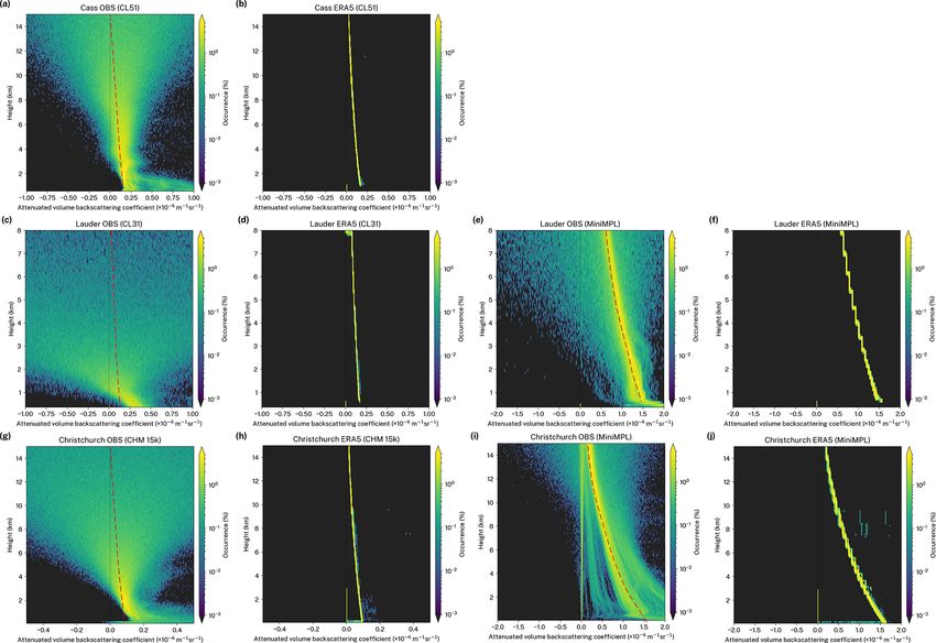
44                                                  P. Kuma et al.: Ground-based lidar processing and simulator framework

Sassen, 2001; Martucci et al., 2010; Costa-Surós et al., 2013;       datasets, and high-resolution model simulations, amongst
Van Tricht et al., 2014; Liu et al., 2015a, b; Lewis et al., 2016;   others. Clouds are one of the most problematic phenomena
Cromwell and Flynn, 2018; Silber et al., 2018), the parti-           in atmospheric models due to their transient nature, high
cle volume backscattering coefficient (Marenco et al., 1997;         spatial and temporal variability, and sensitivity to a com-
Welton et al., 2000, 2002; Wiegner and Geiß, 2012; Wieg-             plex combination of conditions such as relative humidity,
ner et al., 2014; Jin et al., 2015; Dionisi et al., 2018), and       aerosols (presence of cloud condensation nuclei and ice nu-
boundary layer height (Eresmaa et al., 2006; Münkel et al.,          clei), and thermodynamic and dynamic conditions. At the
2007; Emeis et al., 2009; Tsaknakis et al., 2011; Milroy et al.,     same time, clouds have a very substantial effect on the at-
2012; Knepp et al., 2017) can be derived from the attenuated         mospheric shortwave and longwave radiation balance, and
volume backscattering coefficient profile. Lidars equipped           any cloud misrepresentation has a strong effect on other com-
with polarisation or multiple wavelengths can also provide           ponents of the model, limiting the ability to accurately rep-
the depolarisation ratio or colour ratio, respectively, which        resent past and present climate and predict future climate
can be used to infer cloud phase or particle types. Doppler          (Zadra et al., 2018). An improved understanding of clouds
lidars can measure wind speed in the direction of the lidar          and cloud feedbacks is one of the focuses of the Coupled
orientation. ALCs are commonly deployed at airports, where           Model Intercomparison Project Phase 6 (CMIP6) (Eyring
they provide CBH, fog and aerosol observations needed for            et al., 2016), and comparison of model cloud with observa-
air traffic control. Large networks of up to hundreds of li-         tions is one of the key points of the Cloud Feedback Model
dars and ceilometers have been deployed worldwide: Cloud-            Intercomparison Project (CFMIP) (Webb et al., 2017). Satel-
net (Illingworth et al., 2007), E-PROFILE (Illingworth et al.,       lite observations make up the majority of the data used to
2018), PollyNET (Baars et al., 2016), ICENET (Cazorla                evaluate model clouds. These include the following: passive
et al., 2017), MPLNET (Welton et al., 2006) and ARM                  visible and IR low-earth-orbit and geostationary radiome-
(Stokes and Schwartz, 1994; Campbell et al., 2002). The              ters measuring, among others, features such as cloud cover,
purpose of these networks is to observe cloud, fog, aerosol,         cloud-top height (CTH) and cloud-top temperature; passive
air quality, visibility and volcanic ash, provide input to nu-       microwave instruments measuring total column water; and
merical weather prediction (NWP) model evaluation (Hogan             active radars and lidars measuring cloud vertical profiles.
et al., 2001; Illingworth et al., 2007; Morcrette et al., 2012;      Ground-based remote sensing instruments include radars, li-
Warren et al., 2018; Lamer et al., 2018; Hansen et al., 2018b)       dars, ceilometers, radiometers and sky cameras. As pointed
and assimilation (Illingworth et al., 2015b, 2018), and for cli-     out by Williams and Bodas-Salcedo (2017), using a wide
mate studies. These networks are usually composed of multi-          range of different observational datasets including satellite
ple types of ALCs, with Vaisala CL31, CL51, Lufft (formerly          and ground-based observations for general circulation model
Jenoptik) CHM 15k and Droplet Measurement Technologies               (GCM) evaluation is important due to the limitations of each
(formerly Sigma Space and Hexagon) MiniMPL being the                 dataset.
most common. Complex lidar data processing has been set                 Model cloud is commonly represented by the mixing ra-
up on some of these networks. Notably, at the SIRTA site             tio of liquid and ice to the cloud fraction (CF) on every
in France, a lidar ratio (LR) comparable with a lidar sim-           model grid cell and vertical level. In addition, some mod-
ulator (Chiriaco et al., 2018) is calculated as part of the          els provide the cloud droplet effective radius used in radia-
“ReOBS” processing method. Intercomparison and calibra-              tive transfer calculations. Remote sensing observations do
tion campaigns such as CeiLinEx2015 (Mattis et al., 2016)            not match the representation of the atmospheric model fields
and INTERACT-I(-II) (Rosoldi et al., 2018; Madonna et al.,           directly because of their different resolutions, limited field
2018) have been performed. Lidar data processing involves            of view (FOV) and attenuation by atmospheric constituents
a number of tasks such as re-sampling, calibration, noise re-        before reaching the instrument’s receiver. Instrument simula-
moval and cloud detection. Some of these are implemented             tors bridge this gap by converting the model fields to quanti-
in the instrument firmware of ALCs. This, however, means             ties which emulate those measured by the instrument, which
that the lidar attenuated volume backscattering coefficient          can then be compared directly with observations. One such
and detected cloud and cloud base are not comparable be-             collection of instrument simulators is the CFMIP Observa-
tween different instruments. In most cases the algorithms are        tion Simulator Package (COSP) (Bodas-Salcedo et al., 2011;
not publicly documented, making it impossible to compare             Swales et al., 2018), which has been used for more than
the data with values from a model or a lidar simulator with-         a decade for the evaluation of models using satellite, and
out a systematic bias.                                               more recently ground-based, observations. The simulators
   Atmospheric model evaluation is an ongoing task and a             in COSP include the following: active instruments (space-
critical part of the model improvement process (Eyring et al.,       borne and ground-based radars) such as the Cloud Profil-
2019; Hourdin et al., 2017; Schmidt et al., 2017). Tradi-            ing Radar (CPR) on CloudSat (Stephens et al., 2002) and
tionally, various types of observational and model datasets          the Ka-band ARM Zenith Radar (KAZR); lidars such as
have been utilised – weather and climate station data, upper-        Cloud–Aerosol Lidar Orthogonal Polarization (CALIOP) on
air soundings, ground-based and satellite remote sensing             CALIPSO (Winker et al., 2009), the Cloud–Aerosol Trans-

Geosci. Model Dev., 14, 43–72, 2021                                                     https://doi.org/10.5194/gmd-14-43-2021
P. Kuma et al.: Ground-based lidar processing and simulator framework                                                          45

port System (CATS) on ISS (McGill et al., 2015) and the At-         Here, we provide an overview of the ALCF (Sect. 2)
mospheric Lidar (ATLID) on EarthCARE (Illingworth et al.,         and describe the supported ALCs, reanalyses and models
2015a); and spaceborne passive instruments such as ISCCP          (Sect. 3), the lidar simulator (Sect. 4), and the observed and
(Rossow and Schiffer, 1991), MODIS (Parkinson, 2003) and          simulated lidar data processing steps (Sect. 5). Later, we
MISR (Diner et al., 1998). The more recent addition of            present a set of case studies at three sites in New Zealand
ground-based radar (Zhang et al., 2018) and lidar (Chiri-         (NZ) (Sect. 6) to demonstrate the value of this new tool.
aco et al., 2018; Bastin et al., 2018) opens up new possi-        Lastly, we present the results of the case studies in Sect. 7.
bilities to use the large amount of remote sensing data ob-
tained from ground-based active remote sensing instruments.
In practice, ground-based observational remote sensing data       2   Overview of operation of the Automatic Lidar and
are not straightforward to use without a substantial amount of        Ceilometer Framework (ALCF 1.0)
additional processing. Some previous studies have also com-
                                                                  The ALCF performs the necessary steps to simulate the
pared models and ground-based radar and lidar observations
                                                                  ALC attenuated volume backscattering coefficient based on
without the use of an instrument simulator (Bouniol et al.,
                                                                  four-dimensional atmospheric fields from reanalyses, NWP
2010; Hansen et al., 2018a), though for the reasons identified
                                                                  models and GCMs, as well as to transform the observed
above this is not advisable.
                                                                  raw ALC attenuated volume backscattering coefficient pro-
   In this study we introduce a software package called the
                                                                  files to profiles comparable with the simulated profiles. It
Automatic Lidar and Ceilometer Framework (ALCF) for
                                                                  does so by extracting two-dimensional (time × height)
evaluating model cloud using ALC observations. It extends
                                                                  profiles from the model data, performing radiative trans-
and integrates the COSP lidar simulator (Chiriaco et al.,
                                                                  fer calculations based on a modified COSP lidar simula-
2006; Chepfer et al., 2007; Chepfer et al., 2008) with pre-
                                                                  tor (Sect. 4), absolute calibration and re-sampling of the
and post-processing steps and allows the simulator to be run
                                                                  observed attenuated volume backscattering coefficient to a
offline on model output instead of having to be integrated
                                                                  common resolution, and performing comparable cloud de-
inside the model. This makes it possible to compare ALC
                                                                  tection on the simulated and observed attenuated volume
data at any location without having to run the model with a
                                                                  backscattering coefficient. The framework supports multiple
specific configuration. Multiple ALCs, reanalyses and model
                                                                  common ALCs (Sect. 3.1), reanalyses and models (Sect. 3.2).
output formats are supported. The original COSP lidar sim-
                                                                  The schematic in Fig. 1 illustrates this process as well as
ulator was extended with Rayleigh, Mie and ice crystal scat-
                                                                  the ALCF commands which perform the individual steps.
tering at multiple lidar wavelengths. Observational ALC data
                                                                  The following commands are implemented: model, simu-
from a number of common instruments can be processed by
                                                                  late, lidar, stats and plot. The commands are normally
re-sampling to a common resolution, removing noise, detect-
                                                                  executed in a sequence, which is also implemented by a
ing cloud and calculating statistics. The same steps can be
                                                                  meta-command auto that is equivalent to executing a se-
performed on the simulated lidar data from the model (the
                                                                  quence of commands. The commands are described in de-
output of running COSP on the model data), allowing for
                                                                  tail in the technical documentation available online at https:
one-to-one comparison of model and observations. A par-
                                                                  //alcf-lidar.github.io (last access: 1 January 2021), on Zenodo
ticular focus of our work was on applying the same pro-
                                                                  at https://doi.org/10.5281/zenodo.4411633 and in the Sup-
cessing steps to the observed and simulated attenuated vol-
                                                                  plement. The physical basis is described here.
ume backscattering coefficient in order to avoid biases. The
                                                                     The model command extracts two-dimensional profiles
ALCF is made available under an open-source licence (MIT)
                                                                  of cloud liquid and ice content (and other thermodynamic
at https://alcf-lidar.github.io (last access: January 2021) and
                                                                  fields) from the supported NWP model, GCM and reanalysis
as a permanent archive of code and technical documentation
                                                                  data (model data in Fig. 1) at a geographical point along a
on Zenodo at https://doi.org/10.5281/zenodo.4411633.
                                                                  ship track or a flight path. The resulting profiles are recorded
   A relatively small amount of other open source code is
                                                                  as NetCDF files. Section 3.2 describes the supported reanal-
available for ALC data processing. A lidar simulator has
                                                                  yses and models. The model data can either be in one of the
been developed as part of the Goddard Satellite Data Simu-
                                                                  supported model output formats, or a new module for read-
lator Unit (G-SDSU) (Matsui, 2019), a package based on the
                                                                  ing arbitrary model output can be written provided that the
instrument simulator package SDSU (Masunaga et al., 2010).
                                                                  required atmospheric fields are present in the model output.
The Community Intercomparison Suite (CIS) (Watson-Parris
                                                                  The required model fields are per-level specific cloud liquid
et al., 2016) allows for subsetting, aggregation, co-location
                                                                  water content, specific cloud ice water content, cloud frac-
and plotting of mostly satellite data with a focus on model–
                                                                  tion, geopotential height, temperature, surface-level pressure
observation intercomparison. The STRAT lidar data process-
                                                                  and orography. No physical calculations are performed by
ing tools are a collection of tools for conversion of raw ALC
                                                                  this command. The atmospheric profiles are extracted by a
data, visualisation and feature classification (Morille et al.,
                                                                  nearest-neighbour selection.
2007).

https://doi.org/10.5194/gmd-14-43-2021                                                   Geosci. Model Dev., 14, 43–72, 2021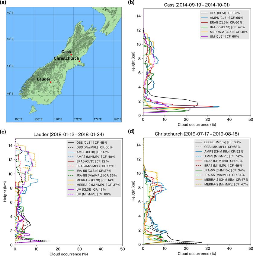
46 P. Kuma et al.: Ground-based lidar processing and simulator framework
Figure 1. (a) Scheme showing the operation of the ALCF and (b) the processing commands.
The simulate command runs the lidar simulator described 3 Supported input data: instruments, reanalyses and
in Sect. 4 on the extracted model data (the output of the models
model command) and produces simulated attenuated vol-
ume backscattering coefficient profiles. This command runs
the COSP-derived lidar simulator, which performs radiative 3.1 Instruments
transfer calculations of the laser radiation through the atmo-
sphere. The resulting simulated attenuated volume backscat-
tering coefficient profiles are the output of this command. The primary focus of the framework is to support common
The lidar command applies various processing algorithms commercial ALCs. Ceilometers are considered the most ba-
to either the simulated attenuated volume backscattering co- sic type of lidar (Emeis, 2010; Kotthaus et al., 2016) intended
efficient (the output of the simulate command) or the ob- as commercial products designed for unattended operation.
served ALC coefficient (lidar data in Fig. 1) (Sect. 5). The They are used routinely to measure CBH, but most instru-
data are re-sampled to increase the signal-to-noise ratio ments also provide the full vertical profiles of the attenuated
(SNR), noise is subtracted, LR is calculated, a cloud mask volume backscattering coefficient. Therefore, they are suit-
is calculated by applying a cloud detection algorithm and able for model evaluation by comparing not only CBH, but
CBH is determined from the cloud mask. Absolute calibra- also cloud occurrence as a function of height. Their compact
tion (Sect. 5.2) can also be applied in this step by multiplying size and low cost make it possible to deploy a large num-
the observed attenuated volume backscattering coefficient by ber of these instruments in different locations or use them in
a calibration coefficient. This is important in order to obtain unusual settings such as mounted on ships (Klekociuk et al.,
unbiased attenuated volume backscattering coefficient pro- 2019; Kuma et al., 2020). Common off-the-shelf ceilome-
files comparable with the simulated profiles. Section 3.1 de- ters are the Lufft CHM 15k and the Vaisala CL31 and CL51.
scribes the supported instruments. The lidar data can be in Some lidars offer higher power and therefore higher SNR, as
one of the supported instrument formats. If the native instru- well as capabilities not present in ceilometers such as dual
ment format is not NetCDF, it has to be converted from the polarisation, multiple wavelengths, Doppler shift measure-
native format with the auxiliary command convert or one ment and Raman scattering. Below we describe ALCs sup-
of the conversion programmes: cl2nc (Vaisala CL31, CL51), ported by the framework and used in our case studies: Lufft
mpl2nc or SigmaMPL (Sigma Space MiniMPL). CHM 15k, Vaisala CL31 and CL51 and Droplet Measure-
The stats step calculates summary statistics from the out- ment Technologies MiniMPL. Table 1 lists selected parame-
put of the lidar command. These include CF, cloud occur- ters of the supported ALCs.
rence by height, attenuated volume backscattering coefficient The Lufft CHM 15k (previously Jenoptik CHM 15k) is a
histograms, and the averages of LR and the backscattering ceilometer operating at a wavelength of 1064 nm (near IR).
coefficient. The maximum range of the instrument is 15.4 km, with a ver-
The plot command plots attenuated volume backscattering tical sampling resolution of 5 m in the first 150 and 15 m
coefficient profiles produced by the lidar command (Figs. 4, above as well as sampling rate of 2 s. The total number of
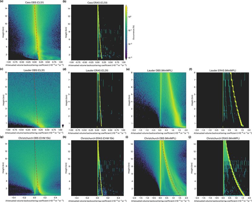
5, 6) and the statistics produced by the stats command: cloud vertical levels is 1024. The wavelength in the near-IR spec-
occurrence (Fig. 3), attenuated volume backscattering coeffi- trum ensures low molecular backscattering. The instrument
cient histograms (Fig. 7) and attenuated volume backscatter- produces NetCDF files containing uncalibrated attenuated
ing coefficient noise standard deviation histograms (Fig. 9). volume backscattering coefficient profiles and various de-
rived variables, although the calibration coefficient is rela-
Geosci. Model Dev., 14, 43–72, 2021 https://doi.org/10.5194/gmd-14-43-2021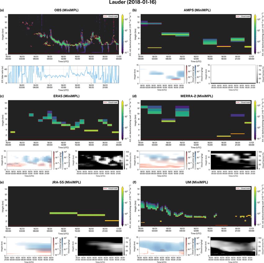
P. Kuma et al.: Ground-based lidar processing and simulator framework                                                                                                        47

Table 1. Table of ALCs and their technical parameters. Power is calculated as pulse × pulse repetition frequency (PRF).

       Instrument        λ (nm)       Laser           Rate1       Res.2       Depol.3       Pulse4       Range5         PRF        Overlap6        Power        FOV7
                                                         (s)       (m)                        (µJ)         (km)        (kHz)            (m)        (mW)         (µrad)
       CHM 15k             1064       Nd:YAG          2–600           5       no                 7–9         15.4         5–7          10008            48         450
       CL31                 910       InGaAs          2–120          10       no                  1.2         7.7           10           708            12         830
       CL51                 910       InGaAs          6–120          10       no                    3        15.4          6.5          2309            20         560
       MiniMPL              532       Nd:YAG          1–900        5–75       yes                3–4         30.0          2.5         20009             9         110
     1 Sampling rate. 2 Vertical (range) resolution. 3 Depolarisation. 4 Pulse energy. 5 Maximum range. 6 Range of full overlap. 7 Receiver field of view. 8 Hopkin et al.
     (2019). 9 Madonna et al. (2018).

tively consistent for different instruments of the model (Hop-                             3.2     Reanalyses and models
kin et al., 2019, Fig. 13).
   The Vaisala CL31 and CL51 are ceilometers operating at a                                Below we briefly describe the reanalyses and models1 used
wavelength of 910 nm (near IR). The maximum range of the                                   in the case studies presented here (Sect. 6). We used pub-
CL31 and CL51 is 7.7 and 15.4 km, and the sampling rate is                                 licly available output from three reanalyses and one NWP
2 and 6 s, respectively. The vertical resolution is 10 m. The                              model. In addition, we performed nudged GCM simulations
total number of vertical levels is 770 and 1540, respectively.                             with high-temporal-resolution output with the Unified Model
The wavelength is characterised by relatively low molecu-                                  (UM). Table 2 lists some of the main properties of the reanal-
lar backscattering (but higher than 1064 nm) and is affected                               yses and models.
by water vapour absorption (Wiegner and Gasteiger, 2015;                                      The Antarctic Mesoscale Prediction System (AMPS)
Wiegner et al., 2019), which can cause additional absorption                               (Powers et al., 2003) is a limited-area NWP model based
of about 20 % in the mid-latitudes and 50 % in the tropics                                 on the polar fifth-generation Pennsylvania State University–
(see also Sect. 5.4). The instruments produce data files con-                              National Center for Atmospheric Research Mesoscale Model
taining uncalibrated attenuated volume backscattering coef-                                (Polar MM5), now known as the Polar Weather Research and
ficients which can be converted to NetCDF (see cl2nc in the                                Forecasting (WRF) model (Hines and Bromwich, 2008). The
“Code and data availability” section). The firmware config-                                model serves operational and scientific needs in Antarctica,
uration option “noise_h2 off” results in a backscatter range                               but its largest grid also covers the South Island of NZ. AMPS
correction being selectively applied under a certain critical                              forecasts are publicly available on the Earth System Grid
range and above this range only if cloud is present (Kot-                                  (Williams et al., 2009). The forecasts are produced on several
thaus et al., 2016, Sect. 3.2). This was the case with our case                            domains. The largest domain D01 used in the presented anal-
study dataset (Sect. 6). We apply a range correction to the un-                            ysis covers NZ and has horizontal grid spacing of approx-
corrected range gates during lidar data processing. The criti-                             imately 21 km over NZ. The model uses 60 vertical levels.
cal range in CL51 is not documented but was determined as                                  The model output is available in 3-hourly intervals initialised
6000 m based on an observed discontinuity.                                                 at 00:00 and 12:00 UTC. The initial and boundary conditions
   The Droplet Measurement Technologies Mini Micro Pulse                                   are based on the Global Forecasting System (GFS) global
Lidar (MiniMPL) (previously Sigma Space MiniMPL and                                        NWP model. AMPS assimilates local Antarctic observations
Hexagon MiniMPL) (Spinhirne, 1993; Campbell et al., 2002;                                  from human-operated stations, automatic weather stations
Flynn et al., 2007) is a dual-polarisation micro-pulse lidar                               (AWS), upper-air stations and satellites.
(meaning that it uses a high pulse repetition rate (PRF) and                                  ERA5 (ECMWF, 2019) is a reanalysis produced by
low pulse power) operating at a wavelength of 532 nm (green                                the European Centre for Medium-Range Weather Forecasts
in the visible spectrum). The maximum range of the instru-                                 (ECMWF) currently available for the time period 1979 to
ment is 30 km. The vertical resolution is 5–75 m and the                                   the present, with a plan to extend the time period to 1950.
sampling rate is 1 s. The shorter wavelength is affected by                                The reanalysis is based on the global NWP model Integrated
stronger molecular backscattering than 910 and 1064 nm.                                    Forecast System (IFS) version CY41R2. It uses a 4D-Var
The instrument can be housed in an enclosure with a scan-                                  assimilation of station, satellite, radiosonde, radar, aircraft,
ning head to provide configurable scanning by elevation an-                                ship-based and buoy data. The model has 137 vertical levels.
gle and azimuth. The instrument produces data files contain-                               Atmospheric fields are interpolated from a horizontal resolu-
ing raw attenuated volume backscattering coefficients which                                tion equivalent to 31 km with 137 model levels on a regular
can be converted to NetCDF containing normalised relative
                                                                                               1 We use the term “reanalysis” when referring to ERA5, JRA-
backscatter (NRB) with the vendor-provided tool SigmaMPL
(see also mpl2nc in the “Code and data availability” section).                             55 and MERRA-2 even though the reanalyses are based on atmo-
                                                                                           spheric models. We use the term “model” when referring to AMPS
                                                                                           and the UM, which are atmospheric models.

https://doi.org/10.5194/gmd-14-43-2021                                                                                     Geosci. Model Dev., 14, 43–72, 2021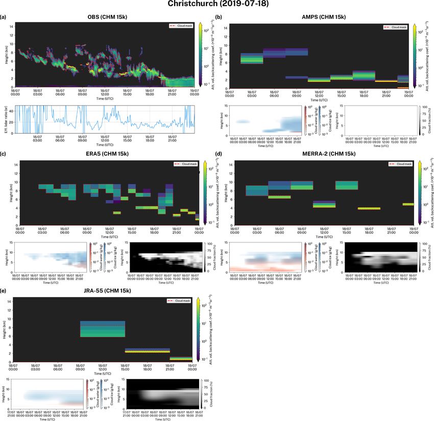
48                                                     P. Kuma et al.: Ground-based lidar processing and simulator framework

Table 2. Reanalyses and models used in the case studies and some of their main properties. The temporal and horizontal grid resolution and
vertical levels listed indicate the resolution of the model output available. The horizontal grid resolution is determined at 45◦ S. The internal
resolution of the model may be different (see Sect. 3.2 for details). The reanalyses and the UM use regular longitude–latitude grids, while
the AMPS horizontal grid is regular in the South Pole stereographic projection.

                        Model and grid         Type           Time          Horizontal                          Vertical
                                                              resolution    grid resolution                      levels
                        AMPS, D01              NWP            3h            0.27◦ × 0.19◦ (21 × 21 km)               60
                        ERA5                   Reanalysis     1h            0.25◦ × 0.25◦ (20 × 28 km)               37
                        JRA-55                 Reanalysis     6h            1.25◦ × 1.25◦ (98 × 139 km)              37
                        MERRA-2                Reanalysis     3h            0.625◦ × 0.50◦ (49 × 56 km)              72
                        UM (GA7.1), N96        GCM            20 min        1.875◦ × 1.25◦ (147 × 139 km)            85

longitude–latitude grid of 0.25◦ and 37 pressure levels, all of            HadISST sea surface temperature (SST) and sea ice dataset
which is made available to end users. In this analysis we use              (Rayner et al., 2003). The model uses 85 vertical levels and
the hourly data on pressure and surface levels.                            a horizontal grid resolution of 1.875◦ × 1.25◦ .
   The Japanese 55-year reanalysis (JRA-55) (Ebita et al.,
2011; Kobayashi et al., 2015; Harada et al., 2016) is a global
reanalysis produced by the Japan Meteorological Agency                     4   Lidar simulator
(JMA) and the Central Research Institute of Electric Power
Industry (CRIEPI) based on the JMA Global Spectral Model                   The COSP lidar simulator, the Active Remote Sensing Simu-
(GSM). The reanalysis is available from 1958 onward. The                   lator (ACTSIM), was introduced by Chiriaco et al. (2006) for
reanalysis is based on the JMA operational assimilation sys-               the purpose of deriving simulated CALIOP measurements
tem. JRA-55 uses a 4D-Var assimilation of surface, upper-                  (Chepfer et al., 2007; Chepfer et al., 2008). The simula-
air, satellite, ship-based and aircraft observations. The model            tion is implemented by applying the lidar equation on model
uses 60 vertical levels and a horizontal grid with a resolution            levels. Scattering and absorption by cloud particles and air
of approximately 60 km. In this analysis we use the 1.25◦ iso-             molecules are calculated using the Mie and Rayleigh theory,
baric analysis and forecast fields interpolated to 37 pressure             respectively. Scattering and absorption by aerosols are not
levels.                                                                    implemented in the presented version, but support is planned
   The Modern-Era Retrospective analysis for Research and                  in the future for models which provide the concentration
Applications (MERRA-2) (Gelaro et al., 2017) is a reanal-                  of aerosols. Therefore, the current focus of the simulator is
ysis produced by the NASA Global Modeling and Assimi-                      solely on cloud evaluation. CALIOP operates at a wavelength
lation Office (GMAO). The reanalysis is based on the God-                  of 532 nm, and calculations in the original COSP simulator
dard Earth Observing System (GEOS) atmospheric model.                      use this wavelength. We implemented a small set of changes
The model has approximately 0.5◦ × 0.65◦ horizontal reso-                  to the lidar simulator to support a number of ALCs with dif-
lution and 72 vertical levels. It performs 3D-Var assimilation             ferent operating wavelengths and developed a parameterisa-
of station, upper-air, satellite, ship-based and aircraft data in          tion of backscattering from ice crystals based on temperature.
6-hourly cycles. In this analysis, we use the MERRA-2 3-                      The lidar equation (Emeis, 2010) is based on the radiative
hourly instantaneous model-level assimilated meteorological                transfer equation (Goody and Yung, 1995; Liou, 2002; Petty,
fields (M2I3NVASM) version 5.12.4 product.                                 2006; Zdunkowski et al., 2007), which relates the transmis-
   The The UK Met Office Unified Model (UM) (Walters                       sion of radiation to scattering, emission and absorption in
et al., 2019) is an atmospheric model for weather forecast-                media such as the atmosphere. The lidar equation assumes
ing and climate projection developed by the UK Met Of-                     that laser radiation passes through the atmosphere where it is
fice and the Unified Model Partnership. The UM is the at-                  absorbed and scattered. A fraction of laser radiation is scat-
mospheric component, called Global Atmosphere (GA), of                     tered back to the instrument and reaches the receiver. Scatter-
the HadGEM3–GC3.1 GCM and the UKESM1 earth system                          ing and absorption in the atmosphere are determined by their
model (ESM). In this analysis we performed custom nudged                   constituents – gases, liquid droplets, ice crystals and aerosol
runs of the UM (Telford et al., 2008) in the GA7.1 configura-              particles. The focus of the current version of the simulator
tion with a 20 min time step and output temporal resolution                is on clouds. For this purpose, the atmospheric model output
on a New Zealand eScience Infrastructure (NeSI)–National                   needed is four-dimensional fields of the mass mixing ratios
Institute of Water & Atmospheric Research (NIWA) super-                    of liquid and ice as well as CF. The lidar equation can be ap-
computer (Williams et al., 2016). The model was nudged to                  plied to these output fields to simulate the backscattered ra-
the ERA-Interim (Dee et al., 2011) atmospheric fields of hor-              diation received by the instrument. Table 3 lists the physical
izontal wind speed and potential temperature as well as the                quantities used in the following sections. Here, we a radiative

Geosci. Model Dev., 14, 43–72, 2021                                                             https://doi.org/10.5194/gmd-14-43-2021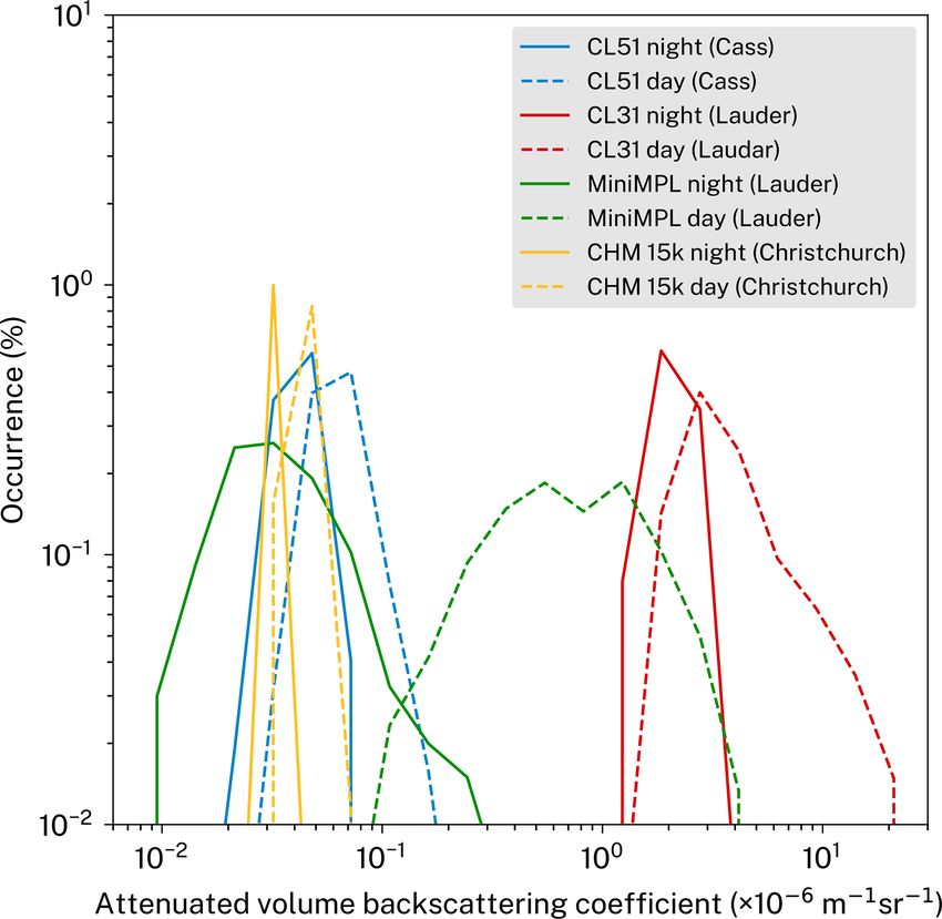
P. Kuma et al.: Ground-based lidar processing and simulator framework                                                                        49

Table 3. Table of physical quantities.

   Symbol      Name                                                        Units        Expression
              Solid angle                                                 sr
   z           Height relative to the instrument                           m
   kB          Boltzmann constant                                          JK−1         kB ≈ 1.38 × 10⁻²³ JK−1
   p           Atmospheric pressure                                        Pa
   T           Atmospheric temperature                                     K
   ρair        Air density                                                 kg m−3
   ρ           Liquid (or ice) density                                     kg m−3
   q           Cloud liquid (or ice) mass mixing ratio                     1
   N           Particle number concentration                               m−3
   αs (αe )    Volume scattering (extinction) coefficient                  m−1          R
   Pπ (θ )     Scattering phase function at angle θ                        1             4π Pπ (θ)d = 4π
   β           Volume backscattering coefficient                           m−1 sr−1     β = αs Pπ (π)/(4π)
   βmol        Volume backscattering coefficient for air molecules
   βp          Volume backscattering coefficient for cloud particles
   η           Multiple-scattering coefficient                             1
   β0                                                                      m−1 sr−1     β 0 = β exp(−2 0z ηαe dz)
                                                                                                         R
               Attenuated volume backscattering coefficient
   S           Lidar ratio (extinction-to-backscatter ratio)               sr           S = αe /β
   S0          Effective (apparent) lidar ratio                            sr           S 0 = Sη
   k           Backscatter-to-extinction ratio                             sr−1         k = 1/S
                                                                           m−4          N = 0∞ n(r)dr
                                                                                              R
   n(r)        Number distribution of particle size
   Qs (Qe )    Scattering (extinction) efficiency of spherical particles   1            αs = Qs πr 2 N , αe = Qe πr 2 N
   Qb          Backscattering efficiency of spherical particles            sr−1         β = QRb πr 2 N
                                                                                        reff = 0∞ r 3 n(r)dr/ 0∞ r 2 n(r)dr
                                                                                                              R
   reff        Effective radius                                            m                                               R
                                                                                        σeff = 0 (r − reff )2 r 2 n(r)dr / 0∞ r 2 n(r)dr
                                                                                                 R∞
   σeff        Effective standard deviation                                m

transfer notation similar to Petty (2006) and the notation of              where S 0 is effective (apparent) LR, a quantity which does
the original lidar simulator (Chiriaco et al., 2006).                      not depend on the multiple-scattering coefficient.
   Below we provide a brief review of LR, Rayleigh and
Mie scattering, calculate LR of cloud droplets at lidar wave-              4.2     Rayleigh and Mie scattering
lengths of the presented instruments, and introduce an empir-
ical parameterisation of LR and the multiple-scattering coef-              The Rayleigh volume backscattering coefficient βmol
ficient of ice crystals based on previous studies.                         (m−1 sr−1 ) in ACTSIM is parameterised by the following
                                                                           equation (Eq. 8 in Chiriaco et al., 2006):
4.1   Lidar ratio                                                                                              −4.09
                                                                                   p                       λ              p
                                                                           βmol =      (5.45 × 10⁻³² )                 =      Cmol , (2)
The lidar ratio S is the extinction-to-backscattering ratio of                    kB T                  550 nm           kB T
atmospheric constituents at the lidar wavelength. It is an
                                                                           where for lidar wavelength λ = 532 nm, Cmol =
important quantity in lidar observations and the lidar sim-
                                                                           6.2446 × 10⁻³² ; kB is the Boltzmann constant
ulator because it determines the amount of attenuation and
                                                                           kB ≈ 1.38 × 10⁻²³ JK−1 , p is the atmospheric pressure
backscattering. LR is not explicitly known from the ob-
                                                                           and T is the atmospheric temperature. We multiply this
served attenuated volume backscattering coefficient. For liq-
                                                                           equation by exp(4.09(log(532) − log(λ))) (where the value
uid cloud droplets at near-IR wavelengths it is relatively con-
                                                                           of λ is in nanometres) to get molecular backscattering
stant at S ≈ 19 sr (Sect. 4.2), while for ice crystals (Sect. 4.3)
                                                                           for wavelengths other than 532 nm, which allows us to
and aerosol it is highly variable. When the lidar signal is fully
                                                                           support multiple commercially available instruments. The
attenuated, and under the assumption that cloud LR is con-
                                                                           strength of molecular backscattering is usually lower than
stant and scattering from clouds is much stronger than molec-
                                                                           backscattering from clouds for the relevant wavelengths.
ular and aerosol scattering, LR can be determined from the
                                                                              The lidar signal at visible or near-IR wavelengths is scat-
observed attenuated volume backscattering coefficient by in-
                                                                           tered by cloud droplets in the Mie scattering regime (Mie,
tegrating it vertically (O’Connor et al., 2004):
                                                                           1908). In the most simple approximation, one can assume
              1                                                            spherical dielectric particles. The scattering from these par-
S 0 = ηS = R ∞ 0 ,                                                (1)
          2 0 β dz                                                         ticles depends on the relative size of the wavelength and the

https://doi.org/10.5194/gmd-14-43-2021                                                               Geosci. Model Dev., 14, 43–72, 2021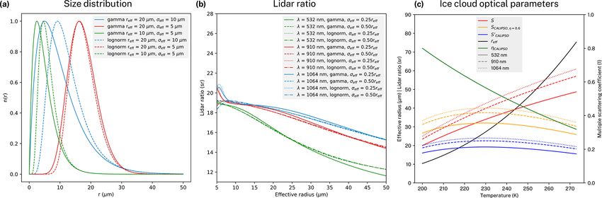
50                                                       P. Kuma et al.: Ground-based lidar processing and simulator framework

(spherical) particle radius r, expressed by the dimensionless                The effective radius reff and effective standard deviation
size parameter x:                                                         σeff are defined by
       2π r                                                                      R∞ 3                   R∞
                                                                                                           (r − reff )2 r 2 n(r)dr
x=          .                                                  (3)                 0 r n(r)dr
        λ                                                                 reff = R ∞ 2        , σeff = 0 R ∞ 2
                                                                                                  2
                                                                                                                                   , (4)
                                                                                   0 r n(r)dr                 0 r n(r)dr
   While the wavelength is approximately constant during
the operation of the lidar2 , the particle size comes from a              where n(r) is the probability density function (PDF) of the
distribution of sizes, typically approximated in NWP mod-                 distribution. Here, we follow Petty and Huang (2011), who
els and GCMs by a gamma or log-normal distribution with                   define the effective variance νeff which relates to σeff by
                                                                                   2 /r 2 . Due to lack of knowledge about the real dis-
                                                                          νeff = σeff
a given mean and standard deviation. Some models provide                                eff
the mean as effective radius reff . If the effective radius is not        tribution of particle radii, it has to be modelled by a theo-
provided by the model, the lidar simulator assumes a value                retical distribution, such as a log-normal or gamma distribu-
reff = 10 µm by default, which is approximately consistent                tion. The original ACTSIM assumes a log-normal distribu-
with global studies of the effective radius (Bréon and Colzy,             tion (Chiriaco et al., 2006) with the PDF:
2000; Bréon and Doutriaux-Boucher, 2005; Hu et al., 2007;
                                                                                             (log r − µ)2

                                                                                   1
Zhang and Platnick, 2011; Rausch et al., 2017; Fu et al.,                 n(r) ∝ exp −                      ,                        (5)
2019). This is different from the default effective radius of                      r              2σ 2
30 µm in the original COSP lidar simulator.                               where µ and σ are the mean and the standard deviation of
   In order to support multiple laser wavelengths, it is nec-             the corresponding normal distribution, respectively. Chiriaco
essary to calculate backscattering efficiency due to scatter-             et al. (2006) use the value of σ = log(1.2) = 0.18 “for ice
ing by a distribution of particle sizes. We use the computer              clouds” (the value for liquid cloud does not appear to be
code MIEV developed by Warren J. Wiscombe (Wiscombe,                      documented). In our parameterisation we used a combina-
1979, 1980) to calculate backscattering efficiency for a range            tion of reff and σeff to constrain the theoretical distribution,
of the size parameter x and integrate for a distribution of               wherein the effective standard deviation σeff was assumed
particle sizes. The resulting pre-calculated LR (extinction-              to be one-fourth of the effective radius reff . This choice is
to-backscatter ratio) as a function of the effective radius is            approximately consistent with σ = log(1.2) = 0.18 at reff =
included in the lidar simulator for fast lookup during the sim-           20 µm (see Table 4, described below). In future updates, the
ulation.                                                                  values could be based on in situ studies of size distribution
   Cloud droplet size distribution parameters are an impor-               or taken from the atmospheric model output if available.
tant assumption in lidar simulation due to the dependence of                 From the expression for the nth moment of the log-normal
Mie scattering on the ratio of the wavelength and particle size                                                  2
                                                                          distribution E[X n ] = exp(nµ + n2 σ2 ) and Eq. (4) we calcu-
(the size parameter x). NWP models and GCMs traditionally                 late reff and σeff of the log-normal distribution:
use the effective radius reff and effective standard deviation
σeff (or an equivalent parameter such as effective variance                      E[r 3 ]              5
νeff ) to parameterise this distribution. Knowledge of the real           reff =         = exp(µ + σ 2 ),                                 (6)
                                                                                 E[r 2 ]              2
distribution is likely highly uncertain due to a large variety                                                                  2 E[r 2 ]
                                                                           2     E[(r − reff )2 r 2 ] E[r 4 ] − 2E[r 3 ]reff + reff
of clouds occurring globally and the limited ability to predict           σeff =                     =
microphysical cloud properties in models. In this section we                           E[r 2 ]                     E[r 2 ]
introduce theoretical assumptions used in the lidar simulator                      exp(4µ + 8σ 2 ) − exp(4µ + 7σ 2 )
                                                                              =
based on established definitions of the effective radius and                               exp(2µ + 2σ 2 )
effective standard deviation as well as two common distribu-
                                                                              = exp(2µ + 6σ 2 ) − exp(2µ + 5σ 2 ).
tions. Edwards and Slingo (1996) discuss the effective radius
                                                                                                                                         (7)
in the context of model radiation schemes, and we will pri-
marily follow the definitions detailed in Chang and Li (2001)                We find µ and σ for given reff and σeff numerically by root-
and Petty and Huang (2011). The practical result of this sec-             finding using the equations above. In practice, we find that
tion (and the corresponding offline code) is pre-calculated               the root-finding converges well for reff between 5 and 50 µm,
backscatter-to-extinction ratios as a function of the effective           which is the range most likely to be applicable in practice.
radius in the form of a lookup table included in the lidar sim-              The gamma distribution follows the PDF:
ulator and used in the online calculations. The offline code is
provided and can be re-used for calculation of the necessary                       (1−3νeff )/νeff          r
                                                                          n(r) ∝ r                 exp −                              (8)
lookup tables for different lidar wavelengths, should the user                                           reff νeff
of the code want to support another instrument.                           (see e.g. Eq. 13 in Petty and Huang, 2011, or Eq. 1 in Bréon
     2 The actual lidar wavelength is not constant and is characterised   and Doutriaux-Boucher, 2005). In this case, the distribution
by a central wavelength and width. The central wavelength may             explicitly depends on reff and σeff and as such does not re-
fluctuate with temperature (Wiegner and Gasteiger, 2015).                 quire numerical root-finding.

Geosci. Model Dev., 14, 43–72, 2021                                                           https://doi.org/10.5194/gmd-14-43-2021
P. Kuma et al.: Ground-based lidar processing and simulator framework 51
Table 4. Table of sensitivity tests for the theoretical distribution assumption, effective radius reff and effective standard deviation σeff of the
cloud droplet size distribution; µ and σ are the mean and standard deviation of a normal distribution, corresponding to the log-normal distri-
bution, numerically calculated from reff and σeff , and µ∗ and σ∗ are the actual mean and standard deviation of the distribution (numerically
calculated).
Distribution reff (µm) σeff (µm) µ σ µ∗ (µm) σ∗ (µm)
log-normal 20 10 2.44 0.47 12.76 6.26
log-normal 20 5 2.84 0.25 17.72 4.43
log-normal 10 5 1.74 0.47 6.40 3.20
Gamma 20 10 9.98 7.00
Gamma 20 5 17.50 4.68
Gamma 10 5 5.00 3.54
Figure 2. (a) Theoretical distributions of cloud droplet radius based on the log-normal and gamma distributions parameterised by multiple
choices of the effective radius reff and effective standard deviation σeff . (b) Lidar ratio (LR) as a function of effective radius calculated for
different theoretical cloud droplet size distributions, laser wavelengths and effective standard deviation ratios. (c) Parameterisation of ice
cloud optical properties as a function of temperature based on Garnier et al. (2015) and Heymsfield (2005). The plot shows LR (S), LR of
CALIPSO calculated using the constant standard processing multiple-scattering coefficient η = 0.6 (SCALIPSO,η=0.6 ), the effective LR of
0
CALIPSO (SCALIPSO ), the effective radius (reff ) and the multiple-scattering coefficient of CALIPSO (ηCALIPSO ) determined by Garnier
et al. (2015). LRs are calculated for three wavelengths of 532 nm (solid line), 910 nm (dashed line) and 1064 nm (dotted line) by scaling with
the colour ratio.
Figure 2a shows the log-normal and gamma distributions
calculated for a number of reff and σeff values, and Table 4
Z∞ Z∞
summarises the properties of these distributions. The actual 4 3 4
mean and standard deviation of the distributions do not nec- qρair = π r ρn(r)dr = πρ r 3 n(r)dr
3 3
essarily correspond well to the effective radius and effective 0 0
standard deviation. Z∞
4
In ACTSIM, the volume extinction coefficient αe is cal- = πρreff r 2 n(r)dr, (10)
culated by integrating the extinction by individual particles 3
0
over the particle size distribution:
where ρ and ρair are the densities of liquid water and air,
Z∞ Z∞
3qρair respectively.
αe = Qe π r n(r)dr ≈ Qe π r 2 n(r)dr = Qe
2
, (9) Likewise, the volume backscattering coefficient from par-
4ρreff
0 0 ticles βp is calculated by integrating backscattering by indi-
vidual particles over the particle size distribution:
assuming approximately constant extinction efficiency Qe ≈
2 (which is approximately true for the interesting range of reff Z∞
and laser wavelengths) and using the relationship between Pπ (π )
R∞ βp = Qs π r 2 n(r)dr, (11)
the cloud liquid mass mixing ratio q and 0 r 2 n(r)dr: 4π
0
https://doi.org/10.5194/gmd-14-43-2021 Geosci. Model Dev., 14, 43–72, 202152 P. Kuma et al.: Ground-based lidar processing and simulator framework
where Qs is scattering efficiency and Pπ (π ) is the scattering rameterised by the asymmetry factor, which is likely insuffi-
phase function at 180◦ . Since the normalisation of n(r) is not cient to give an accurate estimate of backscattering.
known until the online phase of calculation, the backscatter- Because the model ice crystal microphysical and optical
to-extinction ratio from particles kp = β/αe can be calculated properties are not known, they have to be parameterised.
offline instead (the requirement for normalisation of n(r) is A first option is to parameterise the microphysical proper-
avoided by appearing in both the numerator and denomina- ties such as habit and size and theoretically calculate opti-
tor): cal properties. A second option is to directly parameterise
R∞ the optical properties. This appears to be a more practi-
Qs r 2 Pπ (π )/(4π )n(r)dr
kp = βp /αe = 0 R∞
2
. (12) cal choice because of the broad availability of global re-
0 Qe r n(r)dr mote sensing measurements of optical properties from satel-
We pre-calculate this integral numerically for a permis- lites and ground-based lidars compared to relatively scarce
sible interval of reff (5–50 µm) at 500 evenly spaced wave- in situ measurements of ice crystals. Garnier et al. (2015)
lengths and store the result as a lookup table for the online analysed CALIPSO lidar and co-located passive infrared
phase. The integral in the numerator is numerically hard to data from the Imaging Infrared Radiometer (IIR) and de-
calculate due to strong dependency of Pπ (π ) on r. Figure 2b termined a global relationship between temperature, LR and
shows LR as a function of reff , calculated for log-normal the multiple-scattering coefficient at the lidar wavelength of
and gamma particle size distributions with σeff = 0.25reff and 532 nm. The multiple-scattering coefficient is taken as a con-
σeff = 0.5reff . This corresponds to the lookup table we use in stant of 0.6 in the standard CALIPSO data processing, but
the online phase of the lidar simulator. As can be seen in they determined that it is in fact variable between about 0.4
Fig. 2, LR depends only weakly on the choice of the distri- and 0.8. Here, we parameterise LR based on their findings.
bution type and the effective standard deviation ratio. LR varies with the lidar wavelength, a larger part of which is
due to the change in the diffraction peak and a smaller part
4.3 Backscattering from ice crystals is due to the variation of the refractive index (Borovoi et al.,
2014). We use the colour ratio to estimate LR at lidar wave-
Simulation of backscattering from ice crystals is relatively lengths other than 532 nm. A colour ratio of 1064 nm relative
complex compared to backscattering from liquid droplets to 532 nm is commonly estimated for dual-wavelength lidars
due to the very high variability of ice crystal microphys- such as CALIOP. Here, we use a value of 0.8, approximately
ical properties such as habit, size, orientation and surface consistent with the results of Bi et al. (2009) and Vaughan
roughness, all of which affect LR, extinction cross sec- et al. (2010). The effective radius is defined for non-spherical
tion, single-scattering albedo and the multiple-scattering co- particles as reff = 32 IWC
σ , where IWC is the ice water content,
efficient. Common habits include hexagonal plates, hexag- and σ is the volume extinction coefficient of ice. Heymsfield
onal columns, hollow hexagonal columns, droxtals, bullet (2005) summarised the ice crystal effective radius (related to
rosettes, hollow bullet rosettes and aggregates (Baran, 2009; IWC / σ by a factor of 1.64) parameterised as a function of
van Diedenhoven, 2017). Size can be highly variable and bi- temperature based on a number of field studies. We use this
modal with a dependence on temperature and relative humid- relationship for determination of the effective radius. Fig-
ity. Orientation is commonly random or horizontally oriented ure 2c shows the true and effective LR based on Garnier et al.
(often reported with hexagonal ice plates). The surface can (2015) and the effective radius based on Heymsfield (2005),
vary between smooth and rough depending on supersatura- parameterised by the following equations:
tion and crystal age. In general, the Mie theory cannot be
1/T − 1/200
used to simulate backscattering from ice crystals because of S = 20 + (34 − 20) sr, (13)
their irregular shape (Yang et al., 2014). While large crystals 1/230 − 1/200
allow the use of the geometric optics approximation to esti- 1/T − 1/200
η = 0.8 + (0.5 − 0.8) , (14)
mate the optical properties, smaller crystals and diffraction 1/240 − 1/200
by large crystals necessitate the use of more advanced tech- reff = exp (log(16.4) + (log(49.2) − log(16.4))
niques such as the T-matrix method, finite-difference time
1/T − 1/213.15
domain (FDTD), discrete dipole approximation (DDA) and µm, (15)
others, which are generally computationally expensive. Cur- 1/253.15 − 1/213.15
rent global atmospheric models do not normally explicitly where T is atmospheric temperature in Kelvin (K). S follows
parameterise the microphysical properties of cloud ice and Garnier et al. (2015, Fig. 12b), η follows Garnier et al. (2015,
provide only very limited information such as ice mass con- Fig. 9a) and reff follows Heymsfield (2005, Fig. 2), where the
centration and in some cases the effective radius of ice crys- concave and convex shape (respectively) is approximated by
tals in the model output. Radiative transfer schemes of atmo- using 1/T as an argument of the linear approximation, and
spheric models do not explicitly evaluate backscattering (the we use a logarithmic scale of reff in the expression for reff
phase function at 180◦ ) and therefore cannot provide this in- to avoid negative values at low temperature. Figure 2c also
formation to the simulator. Instead the phase function is pa- shows LR when calculated with the assumption of η = 0.6
Geosci. Model Dev., 14, 43–72, 2021 https://doi.org/10.5194/gmd-14-43-2021P. Kuma et al.: Ground-based lidar processing and simulator framework 53
(SCALIPSO,η=0.6 ) as in the standard processing of CALIPSO 4.5 Multiple scattering
data. This corresponds to the empirically found relationship
in Garnier et al. (2015, Fig. 12a) and Josset et al. (2012, Due to a finite FOV of the lidar receiver, a fraction of the laser
Fig. 9) with a local maximum at 225 K. LR at wavelengths radiation scattered forward will remain in the FOV. There-
λ−532 fore, the effective attenuation is smaller than calculated with
other than 532 nm is approximated by 0.8 532 , where λ is
lidar wavelength in micrometres (µm) and 0.8 is the approxi- the assumption that all but the backscattered radiation is re-
mate value of the 1064 nm / 532 nm colour ratio. The param- moved from the FOV and cannot reach the receiver. The
eterisation of LR (S in Fig. 2c) spans about the same range forward scattering can be repeated multiple times before a
of values as reported by Hopkin (2018, Fig. 5.6) (20 to 60 sr) fraction of the radiation is backscattered, eventually reaching
and Yorks et al. (2011) (10 to 60 sr). Based on CALIPSO the receiver. To account for this multiple-scattering effect,
observations, Hu (2007) determined that while the effective the COSP lidar simulator uses a multiple-scattering correc-
LR of global ice clouds at a lidar wavelength of 532 nm is tion coefficient η, by which the volume scattering coefficient
mostly clustered around 17 sr, horizontally oriented plates is multiplied before calculating the layer optical thickness
produce a much lower effective LR below 10 sr caused by (Chiriaco et al., 2006; Chepfer et al., 2007; Chepfer et al.,
specular reflection. These results are close to our parame- 2008). The theoretical value of η is between 0 and 1 and
0
terisation of effective LR (SCALIPSO ). In the current version depends on the receiver FOV and optical properties of the
of the lidar simulator we do not parameterise horizontally cloud. For CALIOP at λ = 532 nm a value of 0.7 is used
oriented plates, but in a future version they could be taken in the COSP lidar simulator. Hogan (2006) implemented a
into account by parameterising their concentration based on fast approximate multiple-scattering code. This code has re-
temperature (Noel and Chepfer, 2010). For the ALCs we use cently been used by Hopkin et al. (2019) in their ceilome-
the same constant value of the multiple-scattering coefficient ter calibration method. They noted that η is usually between
η = 0.7 as for liquid cloud droplets (Sect. 4.5). 0.7 and 0.85 for wavelengths between 905 and 1064 nm. The
ALC simulator presented here does not use an explicit calcu-
4.4 Cloud overlap and cloud fraction lation of η but retains the value of η = 0.7 for cloud droplets.
The code of Hogan (2006), “Multiscatter”, is publicly avail-
Model cloud is defined by the liquid and ice mass mixing ra- able (http://www.met.reading.ac.uk/clouds/multiscatter/, last
tio as well as the cloud fraction in each atmospheric layer. access: 1 January 2021) and could be used in a later version
The lidar simulator simulates radiation passing vertically at of the framework to improve the accuracy of simulated atten-
a random location within the grid cell. Therefore, it is neces- uation and calibration.
sary to generate a random vertical cloud overlap based on the
cloud fraction in each layer, as the overlap is not explicitly
defined in the model output. Two common methods of gener- 5 Lidar data processing
ating overlap are the random and maximum–random overlap
The scheme in Fig. 1 outlines the processing done in the
methods (Geleyn and Hollingsworth, 1979). In the random
framework. The individual processing steps are described be-
overlap method, each layer is either cloudy or clear with a
low.
probability given by CF, independent of other layers. The
maximum–random overlap method assumes that adjacent 5.1 Noise and subsampling
layers with non-zero CF are maximally overlapped, whereas
layers separated by zero CF layers are randomly overlapped. ALC signal reception is affected by a number of sources of
COSP implements cloud overlap generation in the Subgrid noise such as sunlight and electronic noise (Kotthaus et al.,
Cloud Overlap Profile Sampler (SCOPS) (Klein and Jakob, 2016). Range-independent noise can be removed by assum-
1999; Webb et al., 2001; Chepfer et al., 2008). The ALC sim- ing that the attenuated volume backscattering coefficient at
ulator uses SCOPS to generate 10 random subcolumns for the highest range gate is dominated by noise. This is true
each profile using the maximum–random overlap assumption if the highest range is not affected by clouds or aerosol
as the default setting of a user-configurable option. The at- and if contributions from molecular scattering are negligible.
tenuated volume backscattering coefficient profile and cloud The supported instruments have a range of approximately 8
occurrence can be plotted for any subcolumn. Due to the ran- (CL31), 15 (CL51, CHM 15k) and 30 km (MiniMPL). By
dom nature of the overlap, the attenuated volume backscat- assuming that the distribution of noise at the highest level
tering coefficient profile may differ from the observed profile is approximately normal, the mean and standard deviation
even if the model is correct in its cloud simulation. The ran- can be calculated from a sample over a period of time such
dom overlap generation should, however, result in unbiased as 5 min, which is short enough to assume the noise is con-
cloud statistics. stant over this period and long enough to achieve accurate
estimates of the standard deviation. The mean and standard
deviation can then be scaled by the square of the range to
estimate the distribution of range-independent noise at each
https://doi.org/10.5194/gmd-14-43-2021 Geosci. Model Dev., 14, 43–72, 2021You can also read