Engineering Geology Contents lists available at ScienceDirect - University of Glasgow

Engineering Geology 293 (2021) 106288

 Contents lists available at ScienceDirect

 Engineering Geology
 journal homepage: www.elsevier.com/locate/enggeo

Landslide size matters: A new data-driven, spatial prototype
Luigi Lombardo a, *, Hakan Tanyas b, c, Raphaël Huser d, Fausto Guzzetti e, f,
Daniela Castro-Camilo g
a
 University of Twente, Faculty of Geo-Information Science and Earth Observation (ITC), PO Box 217, Enschede, AE 7500, Netherlands
b
 Hydrological Sciences Laboratory, NASA Goddard Space Flight Center, Greenbelt, MD, United States
c
 USRA, Universities Space Research Association, Columbia, MD, United States
d
 King Abdullah University of Science and Technology (KAUST), Computer, Electrical and Mathematical Sciences and Engineering (CEMSE) Division, Thuwal 23955-
6900, Saudi Arabia
e
 Consiglio Nazionale delle Ricerche (CNR), Istituto di Ricerca per la Protezione Idrogeologica (IRPI), via Madonna Alta 126, 06128 Perugia, Italy
f
 Presidenza del Consiglio dei Ministri, Dipartimento della Protezione Civile, via Vitorchiano 2, 00189 Roma, Italy
g
 School of Mathematics and Statistics, University of Glasgow, Glasgow G12 8QQ, UK

A R T I C L E I N F O A B S T R A C T

Keywords: The standard definition of landslide hazard requires the estimation of where, when (or how frequently) and how
Integrated nested Laplace approximation large a given landslide event may be. The geoscientific community involved in statistical models has addressed
(INLA) the component pertaining to how large a landslide event may be by introducing the concept of landslide-event
Landslide hazard
 magnitude scale. This scale, which depends on the planimetric area of the given population of landslides, in
Earthquake
Landslide area prediction
 analogy to the earthquake magnitude, has been expressed with a single value per landslide event. As a result, the
Slope unit geographic or spatially-distributed estimation of how large a population of landslide may be when considered at
Bayesian spatial modelling the slope scale, has been disregarded in statistically-based landslide hazard studies. Conversely, the estimation of
 the landslide extent has been commonly part of physically-based applications, though their implementation is
 often limited to very small regions.
 In this work, we initially present a review of methods developed for landslide hazard assessment since its first
 conception decades ago. Subsequently, we introduce for the first time a statistically-based model able to estimate
 the planimetric area of landslides aggregated per slope units. More specifically, we implemented a Bayesian
 version of a Generalized Additive Model where the maximum landslide size per slope unit and the sum of all
 landslide sizes per slope unit are predicted via a Log-Gaussian model. These “max” and “sum” models capture the
 spatial distribution of (aggregated) landslide sizes. We tested these models on a global dataset expressing the
 distribution of co-seismic landslides due to 24 earthquakes across the globe. The two models we present are both
 evaluated on a suite of performance diagnostics that suggest our models suitably predict the aggregated landslide
 extent per slope unit. In addition to a complex procedure involving variable selection and a spatial uncertainty
 estimation, we built our model over slopes where landslides triggered in response to seismic shaking, and
 simulated the expected failing surface over slopes where the landslides did not occur in the past.
 What we achieved is the first statistically-based model in the literature able to provide information about the
 extent of the failed surface across a given landscape. This information is vital in landslide hazard studies and
 should be combined with the estimation of landslide occurrence locations. This could ensure that governmental
 and territorial agencies have a complete probabilistic overview of how a population of landslides could behave in
 response to a specific trigger. The predictive models we present are currently valid only for the 25 cases we
 tested. Statistically estimating landslide extents is still at its infancy stage. Many more applications should be
 successfully validated before considering such models in an operational way. For instance, the validity of our
 models should still be verified at the regional or catchment scale, as much as it needs to be tested for different
 landslide types and triggers. However, we envision that this new spatial predictive paradigm could be a
 breakthrough in the literature and, in time, could even become part of official landslide risk assessment
 protocols.

 * Corresponding author.
 E-mail address: l.lombardo@utwente.nl (L. Lombardo).

https://doi.org/10.1016/j.enggeo.2021.106288
Received 18 January 2021; Received in revised form 15 May 2021; Accepted 16 July 2021
Available online 24 July 2021
0013-7952/© 2021 The Author(s). Published by Elsevier B.V. This is an open access article under the CC BY license (http://creativecommons.org/licenses/by/4.0/).

L. Lombardo et al. Engineering Geology 293 (2021) 106288

1. Introduction originated from the more general one used by the United Nations
 Disaster Relief Organization (UNDRO) for all-natural hazards, which in
 Landslides are common in the mountains, in the hills, and along high turn was a generalization of the definition used for seismic hazard
costs, where they can pose serious threats to the population, public and (National Research Council, 1991). Fifteen years later, Guzzetti et al.
private properties, and the economy (Kennedy et al., 2015; Petley, 2012; (1999) extended the definition to include the magnitude of the expected
Daniell et al., 2017; Broeckx et al., 2019). To cope with the landslide landslide, and landslide hazard became “the probability of occurrence
problem (Brabb, 1991; Nadim et al., 2006), and in an attempt to mitigate within a specified period of time and within a given area of a potentially
the landslide damaging effects through proper land planning (Kockel­ damaging landslide of a given magnitude”. Today, this remains the most
man, 1986; Brabb and Harrod, 1989; Glade et al., 2005), investigators common and generally accepted definition of landslide hazard.
have long attempted to map landslides (Guzzetti et al., 2012; Mondini A problem with this definition is that, in contrast to other natural
et al., 2021), to quantify landslide susceptibility (Reichenbach et al., hazards—including, e.g., earthquakes (Wood and Neumann, 1931;
2018), intensity (Lombardo et al., 2018b, 2019b, 2020a), and hazard Gutenberg and Richter, 1936), volcanic eruptions (Newhall and Self,
(Varnes and the IAEG Commission on Landslides and Other 1982), hurricanes (Saffir, 1973; Simpson, 1974), floods (Buchanan and
Mass-Movements, 1984; Guzzetti et al., 1999; Fell et al., 2008; Lari et al., Somers, 1976)—no unique measure or scale for landslide magnitude
2014), to evaluate the vulnerability to landslides of various elements at exists (Hungr, 1997a; Malamud et al., 2004b; Guzzetti, 2005). This
risk (Fuchs et al., 2007; Galli and Guzzetti, 2007; van Westen et al., complicates the practical application of the definition (Guzzetti, 2005).
2008), including the population (Dowling and Santi, 2014; Pereira et al., A further complication arises from the use of the same term “landslide”
2017; Salvati et al., 2018), and to ascertain landslide risk, qualitatively to address both the landslide deposit (i.e., the failed mass) and the
(Fell and Harford, 1997, 1997; Reichenbach et al., 2005; Glade et al., movement of slope materials or of an existing landslide mass (Cruden,
2005) or quantitatively (Salvati et al., 2010; Corominas et al., 2014; 1991; Guzzetti, 2005).
Rossi et al., 2019). In the literature, different approaches and metrics were proposed to
 A problem with many of these attempts has always been the inability size or rank the “magnitude” of a single landslide, or a population of
(or at least the difficulty) to measure and predict the size—i.e., depth, landslides—i.e., a number of landslides in a given area resulting from a
length, width, area, volume, and their multiple ratios and dependencies single event or multiple events in a period (Malamud et al., 2004b; Rossi
(Dai and Lee, 2001; Malamud et al., 2004b; Brunetti et al., 2009a; et al., 2010). For single landslides, authors have proposed to measure
Guzzetti et al., 2009; Taylor et al., 2018a)—of the landslides, which are landslide “magnitude” using the size (e.g., area, depth, volume) (Fell,
known to measure, control, or influence landslide magnitude (Keefer, 1994; Cardinali et al., 2002; Reichenbach et al., 2005), velocity
1984; Cardinali et al., 2002; Fuchs et al., 2007), impact (Guzzetti et al., (UNESCO Working Party On World Landslide Inventory, 1995; Cruden
2003; Bout et al., 2018; van den Bout et al., 2021), and destructiveness and Varnes, 1996; Hungr et al., 2014), kinetic energy (Ksu, 1975; Sassa,
(Fell and Harford, 1997; Cardinali et al., 2002), which in turn depend on 1988; Corominas and Mavrouli, 2011), or destructiveness (Hungr,
the landslide types (Hungr et al., 2014). In this work, we propose an 1997b; Reichenbach et al., 2005; Galli and Guzzetti, 2007) of the slope
innovative approach to build statistical models capable of predicting the failure. Alternatively, Cardinali et al. (2002) and Reichenbach et al.
planimetric area of event-triggered landslides (Stark and Hovius, 2001; (2005) proposed to size landslide magnitude based on an empirical
Malamud et al., 2004b; Guzzetti et al., 2012). To test the approach, we relation linking landslide volume and velocity, a proxy for momentum.
construct and validate two models that predict metrics related to the Other possible metrics that can be used to measure the magnitude of a
planimetric area of earthquake-induced landslides (EQILs) (Keefer, single landslide include, e.g., the depth of the landslide mass, the total or
1984, 2013). For the purpose, we exploit the information on the the differential ground displacement caused by the landslide, the
geographical location and planimetric area of 319,086 landslides shown discharge per unit width (for landslides of the flow type), or the mo­
in 25 EQIL inventories available from the global database collated by mentum of the failed mass. This type of kinematic characteristics may be
Schmitt et al. (2017) and Tanyaş et al. (2017)—currently the largest and better suited to inform on the landslide hazard compared to landslides’
most comprehensive repository of information on seismically-triggered area of volume (Corominas et al., 2014). For instance, a large
slope failures, globally (Fan et al., 2019)—together with spatial deep-seated slowly-moving landslide may pose a negligible threat
morphometric and environmental variables in the areas covered by the compared to a small rockfall. In fact, the high velocity of the rockfall
25 EQIL inventories, and on the seismic properties of the triggering could lead to a much larger hazard to local communities or infrastruc­
earthquakes. ture. However, no data of landslide dynamics (e.g., kinetic energy) are
 The manuscript is organized as follows. We begin by giving back­ currently available for large populations of landslides, making the
ground information on the inherent difficulty to predict landslide sizes, landslide area the only directly measurable property for large
including landslide area or other simple geometric measures of landslide inventories.
size (Section 2). Next, we provide the theoretical background for our A few authors have established empirical probability distributions of
statistical models, and of the metrics that we selected to measure the landslide size (or measures thereof) including, e.g., area (Stark and
performance of our models (Section 4). This is followed by a presenta­ Hovius, 2001; Guzzetti et al., 2002; Malamud et al., 2004b; Korup et al.,
tion of the data used to construct and validate our models, including the 2011; Chen et al., 2017; Jacobs et al., 2017), volume (Martin et al.,
target and explanatory variables, and of the adopted terrain mapping 2002; Dussauge et al., 2003; Malamud et al., 2004b; Brunetti et al.,
unit (Section 3). Next, we compare the results of our modelling effort 2009b), area-to-volume (Guzzetti et al., 2009; Larsen et al., 2010; Tang
(Section 5) and we discuss the model outputs in view of their specific et al., 2019), and width-to-length (Parise and Jibson, 2000; Rickli et al.,
and general relevance, and we provide considerations on the impact of 2009; Taylor et al., 2018b) ratios. Moreover, a few authors have
our approach for the modelling of landslide hazard (Section 6). We examined the factors controlling these distributions (e.g., Pelletier et al.,
conclude summarizing the lessons learnt, with a perspective towards 1997; Guthrie and Evans, 2004; Stark and Guzzetti, 2009; Frattini and
possible future research. Crosta, 2013; Korup et al., 2012; Williams et al., 2018; Tanyaş et al.,
 2019b; Jeandet et al., 2019; Bellugi et al., 2021). Some of the established
2. Background distributions were used to estimate landslide magnitude for hazard
 assessment at the catchment scale, where the probability of landslide
 Varnes and the IAEG Commission on Landslides and Other area p(AL), was taken to represent landslide magnitude, e.g., by Guzzetti
Mass-Movements (1984) were the first to define landslide hazard as “the et al. (2005, 2006). However, the use of empirical probability distri­
probability of occurrence within a specified period of time and within a given butions of measures of landslide size has several problems. First, to
area of a potentially damaging landslide” (Fell et al., 2008). This definition establish reliable distributions of, e.g., landslide area or volume, one

 2

L. Lombardo et al. Engineering Geology 293 (2021) 106288

needs large numbers of empirical data, which can only be obtained from landslide area, explaining a large portion of its variability within slope
large and accurate landslide event inventory maps. These data are not units. Nevertheless, as for susceptibility models, the actual size of the
common and difficult, time-consuming, and costly to prepare (Malamud landslides in each mapping unit is irrelevant for the implementation of
et al., 2004b; Guzzetti et al., 2012; Mondini et al., 2021). Second, intensity models, and such models cannot predict the size (e.g., the area
although Malamud et al. (2004b) and Malamud et al. (2004a) have or volume) of the landslides.
argued that their Inverse Gamma distribution, and other similar distri­ In this work, we extend the traditional approaches used to estimate
butions (Stark and Hovius, 2001; Hovius et al., 1997), are general landslide susceptibility, and the more recent approach proposed to es­
(“universal”), and do not depend on the local terrain or the triggering timate landslide intensity, to model the size (area) of the landslides in
conditions, the hypothesis was challenged by, e.g., Korup et al. (2011) any given terrain mapping unit in a landscape. For this purpose, we
and Tanyaş et al. (2018). It is not clear the extent to which a single build statistically-based, spatially-distributed predictive models that
distribution holds outside the geographical area where it was defined. adopt the log-Gaussian probability distribution to explain characteristics
Third, even the availability of reliable empirical distributions of land­ related to the (aggregated) area of landslides in each mapping unit,
slide area or volume does not guarantee that the estimates obtained from namely
the distribution are accurate in all parts of the study area where it was
defined, and specifically in all slopes and sections of a complex land­ • ALmax, the largest landslide in the considered terrain mapping unit;
scape. Fourth, lack of standard methods and tools to properly model the and
probability distributions of landslide sizes hampers the possibility to • ALsum, the sum of all landslide areas in the considered terrain map­
confront empirical distributions obtained for different areas or the same ping unit.
area at different times (Rossi et al., 2012).
 To the best of our knowledge, no model able to capture and predict Further details on how ALmax and ALsum have been extracted from our
the spatial distribution of landslide sizes (or measures thereof) has been dataset is provided in Sections 3.1 and 3.4, whereas a description of how
proposed in the literature. However, for co-seismic landslides, few ex­ these have been modelled is provided in Section 4.
amples do exist where scholars have at least tried to estimate the con­
trolling factors of landslide size. The most common observation points 3. Data
out to a possible relation between distance to rupture zone and landslide
size (e.g., Keefer and Manson, 1998; Khazai and Sitar, 2004; Massey To test our modelling framework, we used information on (i) the
et al., 2018; Valagussa et al., 2019). This implies that larger landslides location and the planimetric area of a large number of landslides caused
are expected to be closer to the fault zone where the influence of ground by earthquakes of different magnitudes in various parts of the world; (ii)
motion is more intense. In fact, Medwedeff et al. (2020) indicated that the morphometric and environmental settings in the same areas where
the contribution of ground motion has a limited control on size of the the EQILs were triggered; and (iii) on the ground shaking conditions
landslides, compared to hillslope relief. Another common observation caused by the earthquakes that triggered the EQILs. In addition, we
suggests that extremely large landslides can be generally associated with selected a type of terrain subdivision into mapping units known to be
structural features (e.g., Chigira and Yagi, 2006; Catani et al., 2016). suited to model and predict landslides spatially.
Such features cannot be taken into account in regional multivariate
analysis because of limited data regarding the discontinuity surfaces 3.1. Earthquake-induced landslide data
(Fan et al., 2019). Other investigators emphasise the control of
ground-motion characteristics (e.g., frequency content, duration) on We obtained information on EQILs searching the largest collection
landslide size (e.g., Bourdeau et al., 2004; Jibson et al., 2004, 2020; (link here) of seismically-induced landslide event inventories currently
Kramer, 1996; Valagussa et al., 2019). For example, Jibson and Tanyaş available (Schmitt et al., 2017; Tanyaş et al., 2017). At the time of the
(2020) demonstrated a positive correlation between landslide size and search (March 2019), this unique source contained cartographic and
magnitude, ground motion duration, and mean period. These hypothe­ thematic information on 64 EQIL inventories caused by 46 earthquakes
ses require further analyses which need strong-motion records gathered that occurred between 1971 and 2016 globally, counting 554, 333
from a very dense accelerometer monitoring network. Nevertheless, we landslides (Fig. 1). To select the inventories best suited for the scope of
lack such spatial detail to examine available earthquake-triggered our work, we adopted two criteria. First, an inventory must have con­
landslide events. This may be the reason why even just explanatory tained information on the (planimetric) area of each of the mapped
models for landslide sizes are so limited in numbers. landslides. Second, the landslides shown in the inventory must have
 Typical, statistically-based, spatially-distributed landslide predictive been associated with an earthquake for which ground motion data were
models attempt to identify “where” landslides may occur in a given available from the U.S. Geological Survey (USGS) ShakeMap system
region based on a set of environmental characteristics known to control, (Worden and Wald, 2016). Applying the two criteria, we selected 25
or condition landslide occurrence, or their lack of occurrence (Reich­ EQIL inventories in the 40-year period between 1976 and 2016, which
enbach et al., 2018). These susceptibility models explain the discrete, collectively encompass 319,086 landslides in 25 study areas in 13 na­
presence/absence of landslides in any given terrain mapping unit, be it, tions, in all continents, except Oceania and Antarctica, and in a broad
e.g., a grid cell, a unique condition unit, a slope unit (SU), or any other range of morphological, geological, tectonic, seismic, and climate set­
terrain subdivision. For this purpose, the models exploit the Bernoulli tings (Fig. 1 and Table S1).
probability distribution to describe the presence/absence (1/0) of With the exception of the 2007 Pisco, Peru, inventory (see Fig. 1 and
landslides (Reichenbach et al., 2018). Therefore, in this context, the size ID 14 in Table S1), prepared using a combination of automated classi­
of the landslides in each terrain mapping unit is irrelevant. fication and manual adjustment techniques (Lacroix et al., 2013), all the
 Recently, Lombardo et al. (2018b) have proposed to estimate the selected inventories were obtained through the systematic, visual
landslide intensity, an alternative measure complementary to landslide interpretation of satellite images and/or aerial photography (Tanyaş
susceptibility, describing the expected number of landslides in any given et al., 2017). For 23 out of the 25 EQIL inventories, showing a total of
terrain mapping unit. To estimate this intensity measure spatially over 303, 269 landslides (95.0% of the total number of landslides), landslides
large and very large areas, the authors built statistically-based, spa­ were mapped as polygons, and the planimetric area of each landslide,
tially-distributed predictive models that adopt the Poisson probability AL, in m2, was calculated in a GIS. For 22 of these inventories, the
distribution to explain the discrete number (0, 1, 2, 3, …) of landslides in polygon showing an individual landslide typically encompasses (i.e., it
any given terrain mapping unit. Moreover, Lombardo et al. (2020a) have does not separate) the landslide source and deposition areas. Only for
shown that the landslide intensity is positively correlated with the the 2015 Gorkha, Nepal, inventory (see Fig. 1 and ID 24 in Table S1) the

 3

L. Lombardo et al. Engineering Geology 293 (2021) 106288

Fig. 1. Map shows locations (yellow dots) of all the earthquakes known to have triggered landslides and reported in the co-seismic landslide database collated by
Schmitt et al. (2017) and Tanyaş et al. (2017) publicly available (https://www.sciencebase.gov/catalog/item/583f4114e4b04fc80e3c4a1a). The cyan dots show all
the earthquakes for which the database above includes one or more corresponding landslide inventories, out of which, the red dots represent the inventories used in
this study. Map uses Equal Earth map projection (EPSG:2018.048, Šavrič et al., 2019). (For interpretation of the references to color in this figure legend, the reader is
referred to the web version of this article.)

source and deposition areas of each landslide were shown separately dichotomous dataset constitute the basic information upon which any
(Roback et al., 2017). For this inventory, to obtain the landslide area AL following model is regressed. In our case, since we do not have to classify
we merged the landslide source and deposition areas. In the 2007 Pisco, the SUs, but rather build a model on the basis of the landslide plani­
Peru (Lacroix et al., 2013) (271 landslides, 0.09%), and the 2013 metric area, we are only interested in the SUs with mapped landslides,
Lushan, China (Xu et al., 2015) (see Fig. 1 and ID 21 in Table S1) (15, where the extent per mapping unit can be computed.
546 landslides, 4.0%), inventories, landslides were shown as points, For this reason, from the initial set of 144, 724 SUs—representing all
corresponding to the known, inferred, or assumed location of the land­ the mapping units combined across the 25 study areas, we extracted a
slide initiation point, with the landslide area listed in a joint, attribute subset of 23, 343 SUs (16.1%, for a total area of about 62, 794 km2)
table. where EQILs have been mapped reporting their planimetric extent. This
 We would like to point out here that several sources of uncertainty subset represents the dataset upon which we will build our modelling
may affect the measurement of landslide areas and further details on this protocol. As for the complementary subset made of 121, 661 SUs
topic will be described in depth in Section 6.3. without known landslides—83.9%, for a total area of about 156,
 216 km2—we separately store this information for it will enter the
 whole procedure only as the prediction target (as explained in Section
3.2. Terrain mapping unit 4.4).

 Among the several possible terrain mapping units used for spatial
landslide modelling (Hansen, 1984; Soeters and van Westen, 1996; 3.3. Morphometric, environmental, and seismic data
Guzzetti et al., 1999; Reichenbach et al., 2018), we selected the “slope
units” (SUs), which are geomorphological and hydrological terrain For our modelling, we used an initial set of morphometric, envi­
subdivisions bounded by drainage and divide lines (Carrara, 1988; ronmental, and ground shaking (seismic) data obtained from a variety of
Alvioli et al., 2016). SUs represent a good geometric description of digital cartographic sources. The data we used can be grouped into three
natural slopes, where most landslides occur. For our work, we exploited main classes, namely:
the same sets of SUs used previously by Tanyaş et al. (2019a) to model
landslide susceptibility, and to predict the spatial occurrence of land­ • terrain morphometric properties, which we obtained from the
slides, in the same 25 study areas. Tanyaş et al. (2019a) generated the SU 1 arcsec × 1 arcsec (approximately, 30 m × 30 m, at the equator)
terrain subdivisions for the study areas (Fig. 1) using r.slopeunits, an SRTM Digital Elevation Model (DEM) (Farr et al., 2007);
open source software for GRASS GIS (GRASS Development Team, 2017) • soil properties, derived from SoilGrids, at about 250 m × 250 m
developed by Alvioli et al. (2016) for the automatic partitioning of a resolution (Hengl et al., 2017);
landscape into SUs. Table S1 lists the main geometric characteristics of • ground motion properties, derived at about 1 km × 1 km resolution
the 144, 724 SUs in the 25 study areas, which collectively cover 219, from the U.S. Geological Survey (USGS) ShakeMap system (Worden
010 km2. and Wald, 2016).
 In consolidated methods to estimate the landslide susceptibility, in­
tensity, and hazard (Reichenbach et al., 2018; Lombardo et al., 2018a; Overall, we initially select 19 covariates, here listed in Table 1. From
Guzzetti et al., 2005), binary datasets are built by assigning to each the SRTM DEM, we obtained nine covariates representing terrain
mapping unit a label indicating the presence/absence of landslides or morphometric properties known to be related to the presence or absence
their count. In this process, mapping units containing the information of of landslides, and specifically EQILs. We computed the Terrain Slope,
slope failures are as important as mapping units where the instability has because steepness is known to balance the retaining and the destabil­
not been observed. As a result, a balanced (Marjanović et al., 2011) or ising forces (Taylor, 1948). Planar and Profile Curvatures influence
unbalanced (Frattini et al., 2010; Lombardo and Mai, 2018) convergence and divergence of shallow gravitational processes and

 4

L. Lombardo et al. Engineering Geology 293 (2021) 106288

Table 1 measures are reciprocal) of the given SU. The first of the two indices is
Summary of our initial covariate set. computed as the maximum distance divided by the SU Area (DSU/ASU);
 Covariate Acronym Reference Unit and the second corresponds to ratio of the maximum distance divided
 √̅̅̅̅̅̅̅̅
 and the root square of the SU Area (DSU / ASU ). Due to the global nature
 Terrain Slope Slope Zevenbergen and Thorne deg
 (1987) of our study, we initially considered also soil physico-chemical param­
 Planar Curvature PLC Heerdegen and Beran 1/m eters derived from SoilGrids, (Hengl et al., 2017). We considered the
 (1982) bulk density for it expresses the weight of the soil draping over the
 Profile Curvature PRC Heerdegen and Beran 1/m
 underlying rock and thus controls the failure mechanism (Adams and
 (1982)
 Vector Ruggedness VRM Sappington et al. (2007) unitless Sidle, 1987; Cheng et al., 2012). Similarly, the soil depth to the bedrock
 Measure expressed the thickness of material that can potentially fail, where the
 Topographic Wetness TWI Beven and Kirkby (1979) unitless thicker the failed soil column the larger the landslide is expected to be
 Index (Lombardo et al., 2016; Lagomarsino et al., 2017). As for the soil clay
 Terrain Relief Intensity Relief Int Jasiewicz and Stepinski m
 content, this property should carry the signal of potentially swelling soils
 (2013)
 Terrain Relief Range Relief Jasiewicz and Stepinski m (Khaldoun et al., 2009).
 Range (2013) Two seismically-related covariates provide spatially-distributed
 Terrain Relief Variance Relief Var Jasiewicz and Stepinski m ground shaking characteristics for the 25 earthquakes that caused the
 (2013)
 EQILs in our study areas, namely, the microseismic intensity, MI (Wald
 Distance to Stream D . stream e.g., Samia et al. (2020) m
 Landform Classification LC MacMillan and Shary unitless
 et al., 2012); and the peak ground acceleration (PGA), expressed in units
 (2009) of gravity (g) at 1 km × 1 km resolution (PGA, Wald et al., 1999). These
 Slope Unit Area ASU Lombardo et al. (2020b) m2 deterministic estimates of the ground motion represent the severity of
 Slope Unit Maximum DSU Castro Camilo et al. (2017) m ground shaking contributes to the destabilising forces (e.g., Nowicki
 Distance
 et al., 2014; Kritikos et al., 2015; Meunier et al., 2007).
 Slope Unit Elongation D/A Castro Camilo et al. (2017) unitless
 Index 1 We remind here that the properties listed above are computed for
 Slope Unit Elongation
 √̅̅̅̅
 D/ A Castro Camilo et al. (2017) unitless grid cells. As we opt for a different mapping unit (see Section 3.2), each
 Index 2 property is pre-processed to aggregate the lattice information to the
 Bulk Density BD Hengl et al. (2019) kg m− 3
 chosen units (see Section 3.4). Also, we chose a large set of properties to
 Depth to Bedrock DB Shangguan et al. (2017) m
 Clay Fraction CFC Wan and Wang (2018) g/
 incorporate as much information as possible. Nevertheless, our model­
 Concentration g × 100 ling protocol will feature a variable selection step aimed at removing
 Peak Ground PGA Wald et al. (1999) gn non-informative or redundant properties (see Section 4).
 Acceleration
 Microseismic Intensity MI Wald et al. (2012) unitless
 3.4. Pre-processing strategy

overland flows (Ohlmacher, 2007). The Vector Ruggedness Measure We used landslide area as our dependent (target) variable, and we
(Sappington et al., 2007) is a proxy for terrain roughness (Amatulli et al., measured the size of each landslide as the planimetric area of the
2018) and Topographic Wetness Index is a function of the local slope polygon encompassing it, i.e., landslide size = AL. This information was
and of the upstream contributing area that quantifies the topographic then aggregated per SU and expressed on the natural logarithmic scale, i.
control on hydrological processes (Grabs et al., 2009). We computed e., log(AL). Specifically, we prepared two landslide datasets, which we
three possible realizations of the Terrain Relief namely intensity, range, used to construct two different models. For our first model (“Max
and variance (Stepinski and Jasiewicz, 2011). These topographic rep­ model”), we computed the maximum area of all the landslides included
resentations are meant to carry the signal of gravitational potential in each slope unit, ALmax. For our second model (“Sum model”), we
energy across the landscape. The idea is that, taking aside the role of selected the sum of the areas of all the landslides per slope unit, ALsum.
other predisposing factors, a location with a higher relief than another We provide a graphical sketch of our aggregation scheme in
also has a higher potential energy. As a result, the same potential energy Figure S1, and we refer to the Supplementary Material for a more detail
is converted into kinetic energy if a landslide occurs, hence the resulting description. For conciseness in the main text, we have extracted two
runout should be larger than the theoretical runout of a landslide failed metrics ALmax and ALsum, which represent the maximum landslide size
with a lower relief. The relief intensity is computed as the average dif­ per SU and the sum of all landslide sizes per SU. They will represent the
ference between the elevation of a grid-cell and those included in a prediction target of our model.
neighbourhood that we chose within a diameter of 1 km. Conversely, the In addition to the preparatory steps for the target variable, the set of
relief range is expressed as the difference between the minimum and covariates we listed in Section 3.3 have also been preprocessed. For each
maximum elevations within the same circle. Furthermore, the relief morphometric, soil and seismic property, we computed the mean and
variance expressed the variability of the elevation values within the standard deviation of all the grid cells contained in a SU. Conversely, we
same circle. We also calculate the distance to streams as the Euclidean assigned to each slope unit the signal of the Landform class with the
distance from each 30 m × 30 m grid cell to the closest streamline. We largest extent. We stress here that this step may smooth out the signal of
note here that the parameterization used to extract the river network has less present Landform classes although they may still contribute to the
been kept consistent across each of the 25 study areas. The last covariate failure initiation.
we obtained from the DEM consists of Landforms (or Landform Classes). In Fig. 2 we show the distribution of few covariates we computed, for
These are represented by five landforms, from L1 to L5, representing flat each of the 25 study areas. Notably, most of them are distributed
topographies in L1, foot slope and valley in L2, spur and hollow in L3, differently among study sites. Therefore, to respect the unity of each site,
slope, ridge, shoulder in L4 and summit in L5. In addition to the in our modelling scheme we introduced an additional covariate
mentioned morphometric covariates, we selected four additional cova­ expressing the given earthquake. In doing so, we assigned an earthquake
riates describing the geometric properties of our landscape partitioning ID to each slope unit. Further details on how this covariate is used in our
into SUs, namely: the slope unit area, ASU; the maximum distance be­ model are provided in Section 4.
tween any given pairs of points within a SU, a measure of the SU elon­
gation, DSU. From these two geometrical properties, we compute two
shape indices both indicating the elongation or circularity (these

 5

L. Lombardo et al. Engineering Geology 293 (2021) 106288

Fig. 2. Distribution summary of nine example covariates, for each of the earthquakes under consideration. Notably, the units along the abscissas have been
transformed into integers for pure graphical purposes.

 6

L. Lombardo et al. Engineering Geology 293 (2021) 106288

4. Modelling and inference Table 2
 Summary of (only) the selected covariates for both models. In the second col­
 In this section, we present the statistical models assumed to be umn, RW1 refers to random walks of order 1, while RI refers to random
capable of fitting and predicting the spatial distribution of observed intercepts.
ALmax and ALsum, which will also be used to predict unobserved landslide Fixed effects Random effects
sizes (i.e., ALmax and ALsum for a SU with no landslide). Below we provide √̅̅̅̅
 RW1: Mean slope
 Area SU, D/ A, Relief range (mean and sd),
details in terms of the theoretical (Bayesian) framework, the model
 Distance to streams (mean and sd), RI: Landform and
structure and components, as well as the computational aspects of the Sd of slope, VRM (mean and sd), Earthquake inventories
inference approach. PLC (mean and sd), PRC (mean and sd),
 TWI (mean and sd), MI (mean and sd)

4.1. Statistical modelling
 we assume that the random non-linear effect fl(⋅), defined on zl, satisfies
 Here, we describe our modelling framework, which we adopt to /
understand the (possibly non-linear) effect of the explanatory variables Δl,j = fl (zl,j ) − fl (zl,j− 1 ) ∼ (0, 1 κl ),
over the landslide size. We assume that landslide sizes in the considered
terrain mapping unit s, follow a log-Gaussian distribution with an ad­ then fl(⋅) is a normal random walk of order 1 with precision parameter
ditive structure in the mean and a site-specific variance. The mean is our κl > 0, which controls the “smoothness” of the random walk. Note that
main object of interest, and we would like to describe it accurately. We since fl(zl,j) = fl(zl,j− 1) + Δl,j, at each covariate level j, then fl(zl,j) is ob­
mathematically formalise our previous assumption as follows: let AL(s) tained as a displacement of random length and direction from the pre­
be the landslide size at slope unit s ∈ , where represents all the study vious value fl(zl,j− 1). The dependence induced by this type of
area. AL(s) can be either the largest possible landslide (ALmax) or the sum construction is particularly useful when few values of the original co­
of landslide sizes (ALsum) over the considered mapping unit. Then, variate xl are contained in a particular bin.
 Random intercept or independent and identically distributed
log{AL (s)} ∼ (μ(s), 1/τ), Gaussian random effect models (iid models) are one of the simplest ways
 ∑M ∑
 L
 (1) to account for unstructured variability in the data. For every slope unit
 μ(s) =α+ βm xm (s) + fl (zl (s)),
 m=1 s ∈ , the precision matrix of iid random effects is γ(s) × I where I de­
 notes the identity matrix and γ(s) ~ Gamma(1, 10− 5) a priori. As shown
 l=1

where: in Table 2, we used iid models for Landform and Earthquake inventory.

 • τ = 1/σ2 > 0 is the precision parameter (reciprocal of the variance)
 that measures the concentration of all values log {AL(s)}, s ∈ , 4.2. Uncertainty quantification and the bootstrap
 around their mean μ(s). As mentioned before, our main focus is on
 the mean of the landslide sizes rather than their variances. Therefore, The modelling approach presented above describes landslide sizes
 we assume a reference prior distribution for τ, which means that the through a set of covariates at each specific slope unit, without taking
 prior is guaranteed to play a minimal role in the posterior distribu­ into account possible spatial dependence between slope units in the
 tion (Gelman et al., 2013). Specifically, we consider a vague prior by same event. A proper spatial model should include interactions between
 assuming that τ ~ Gamma(1, 5 × 10− 5) a priori, so that the precision slope units, which in statistical terms implies defining a covariance
 is centered at 20,000 and has a huge variance of 4 × 108. structure for all the 22,343 non-missing slope units. Although it is
 • α is a global intercept, possible to define such structures using a neighbouring approach where
 • the coefficients (β1, …, βM)T quantify the fixed effects of the chosen only close-by slope units will interact, and therefore the associated
 linear covariates {x1(s), …, xM(s)} on the mean response, and covariance matrix might be less dense, the high-dimensionality of our
 • {f1(⋅), …, fL(⋅)} is a collection of functions that characterize non- data prohibits us from fitting such a model. Alternatively, we could have
 linear effects defined in terms of a set of bins {z1, …, zL}. These separate models for each of the 25 inventories and define the covariance
 are explained below. structure locally. However, model comparison would be challenging, as
 not all covariates might have the same effect over all the events.
 We adopt a Bayesian approach, and therefore assume that the model In terms of statistical estimation, not addressing the spatial depen­
coefficients βm and fl(⋅), (m = 1, …, M, l = 1, …, L) are unknown and dence between slope units mainly affects the uncertainty of the esti­
random, with a joint Gaussian distribution a priori. This modelling mates, i.e., the credible intervals. Pointwise estimates remain mostly
approach corresponds to the class of latent Gaussian models, which in­ unchanged. To assess the uncertainty of parameter estimates, we here
cludes a wide variety of commonly applied statistical models (Rue et al., use a parametric bootstrap procedure accounting for spatial dependence
2017; Hrafnkelsson et al., 2020; Jóhannesson et al., 2021). To identify in the model residuals. The Bootstrap is a resampling method that can be
the covariates that may enter to the log(ALmax) or log(ALsum) models in used to assign measures of accuracy to estimates. Our parametric
the form of linear or non-linear predictors, we conducted a model se­ Bootstrap is constructed as follows: for any of the two models, we
lection. The selection was based on the Watanabe-Akaike information compute the model residuals (i.e., we subtract to the observed values the
criterion (WAIC; Watanabe, 2010, 2013) and the Deviance information fitted values, log(AL )(s) − ̂
 μ (s)). Then, we fit a spatial model to the re­
criterion (DIC; Spiegelhalter et al., 2002), which measure a model's siduals of each inventory separately (i.e., treating inventories as inde­
goodness-of-fit, while penalizing its complexity, in order to favour pendent). We then generate 300 residual Bootstrap samples using the
parsimonious models and prevent overfitting. Lower values of these fitted spatial model. To express these samples in the scale of the data, we
criteria lead to better models. For each covariate that was linearly add back the fitted values ̂ μ (s), given rise to 300 Bootstrap samples of
included in the models, we tested whether a non-linear random effect for landslide sizes. Finally, we fit the model in (1) to each one of these
the covariate would significantly improve the model. For both response samples, for both models. The spatial model fitted to the residuals cor­
variables, the final models include the same linear and non-linear responds to a stationary isotropic Gaussian process with an exponential
random effects. The latter ones take the form of random intercepts covariance function (see, e.g., Cressie, 2015, Section 2.3). The Bootstrap
and random walks of order 1 (see Table 2). Random walks of order 1 is essential for accurate quantification of the uncertainty, as, without it,
(RW1) can be defined as follows: for any continuous covariate xl = xl(s), uncertainty estimates might be too optimistic, i.e., parameter credible
let zl = (zl,a , …, zl,Kl )T be a discretisation of xl into Kl equidistant bins. If intervals might be too narrow in both models.

 7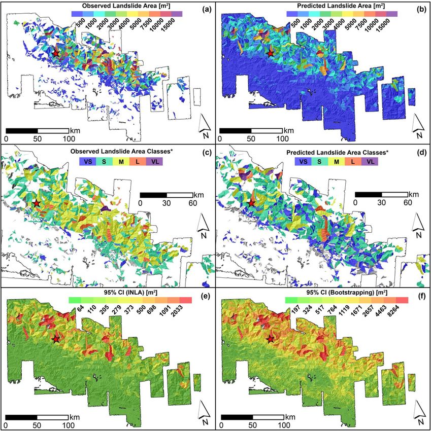

L. Lombardo et al. Engineering Geology 293 (2021) 106288

4.3. Bayesian inference with R-INLA P1 , …, P| | } should be uniformly distributed in (0, 1). The uniformity
 of the PIT values is a necessary condition for the prediction to be
 Bayesian inference is typically performed using computationally perfect (Gneiting et al., 2007) and any deviation from uniformity,
expensive approaches such as Markov chain Monte Carlo (MCMC). Here, implies a decrease in performance.
we overcome these computational costs using the integrated nested • Plot of observed vs. fitted values: In such a plot, we can see how
Laplace approximation (INLA; Rue et al., 2009). When exploiting INLA, much the fitted values deviate from the actual observed landslide
the posterior distribution of the parameters of interest are approximated areas. A model with a reasonable performance should produce values
using numerical methods, which makes it possible to compute the aligned with the main diagonal (i.e., the 45◦ line).
required quantities in a reasonable amount of time. The INLA method­ • Probability coverage: given a probability α ∈ (0, 1), we compute
ology is conveniently implemented in the R-INLA package (Bivand and the proportion of times that a (1− α)100 % credible interval contains
Piras, 2015) and we use it to obtain an accurate approximation of pos­ the observed data. If the underlying model is adequate, then the
terior marginal densities of interest, such as those for μ(s) and the pa­ computed proportion (usually called sample coverage) should be
rameters introduced in Section 4.1. close to (1− α)100 % (the nominal coverage). In practice, the
 Bayesian methodology allows us to simulate from the posterior dis­
4.4. Landslide area simulation tribution in order to compute as many credible intervals as desired.
 For a readership who is unacquainted with the coverage concept,
 The R-INLA package offers built-in functions to compute posterior below we provide a brief and simple explanation. Using posterior
samples even at locations where we do not have observations. In other simulations, we construct 5000 estimates for each observed AL value.
words, using the model fitted to the complete dataset, we can infer the Then, for each AL, we compute sample p-quantiles, with p = {0.025,
distribution of each missing landslide size. Internally, R-INLA treats 0.05, 0.075, …, 0.950, 0.975} (a sequence from 0.025 to 0.975 with
missing values as values that we need to predict. Therefore, if we pro­ steps of size 0.025). These sample quantiles allow us to construct
vide the set of explanatory variables accompanying the missing land­ credible intervals of sizes (1 − α)100 % = {10 % , 15 % … , 90 % ,
slide areas, R-INLA will use the fitted model to predict (or fill in) the 95 % }. Then, we count how many times the observed AL values fell
missing values. In practice, R-INLA performs model fitting and predic­ within these intervals. If the model is adequate, for a credible in­
tion at the same time, producing all the required results in a short terval of size (1− α)100 % the number of times the observed AL is
amount of time. Here, we generated 5000 posterior samples for each contained should be close to (1− α)100 %. For instance, a 95%
missing landslide area. These posterior distributions are summarized in credible interval should contain 95% of the observed AL values.
term of their mean and 95% credible intervals. Therefore, if we plot the nominal coverage vs. the sample one, a
 To put it simply, in a Bayesian framework, the estimation of the reasonable model will show points aligned with the 45◦ line.
posterior regression coefficients consists of a distribution of possible
values. Therefore, by sampling at random each distribution for the effect 5. Results
of each covariate, it is possible to statistically simulate a given process.
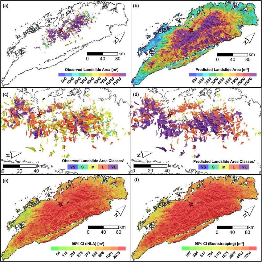
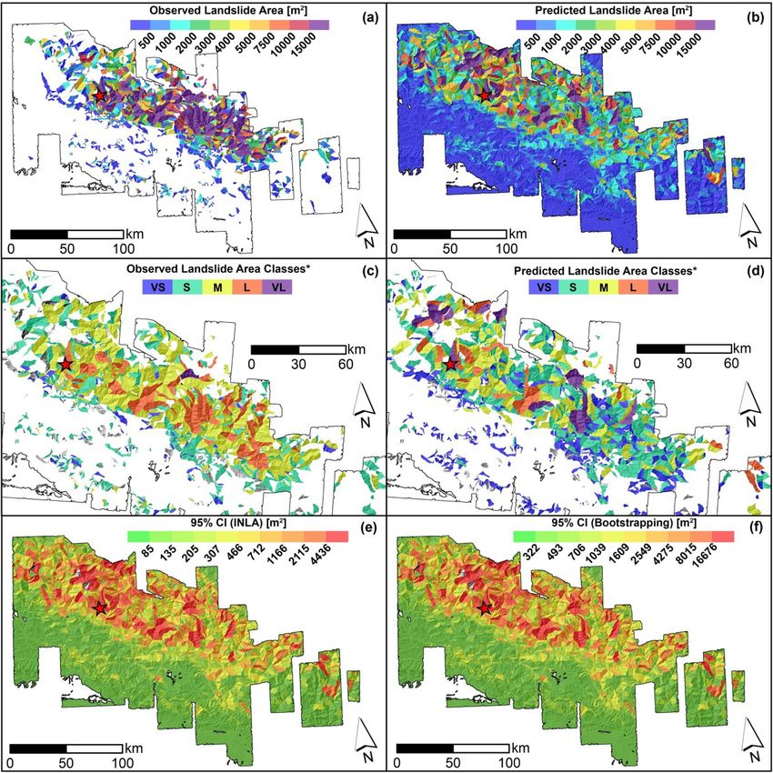
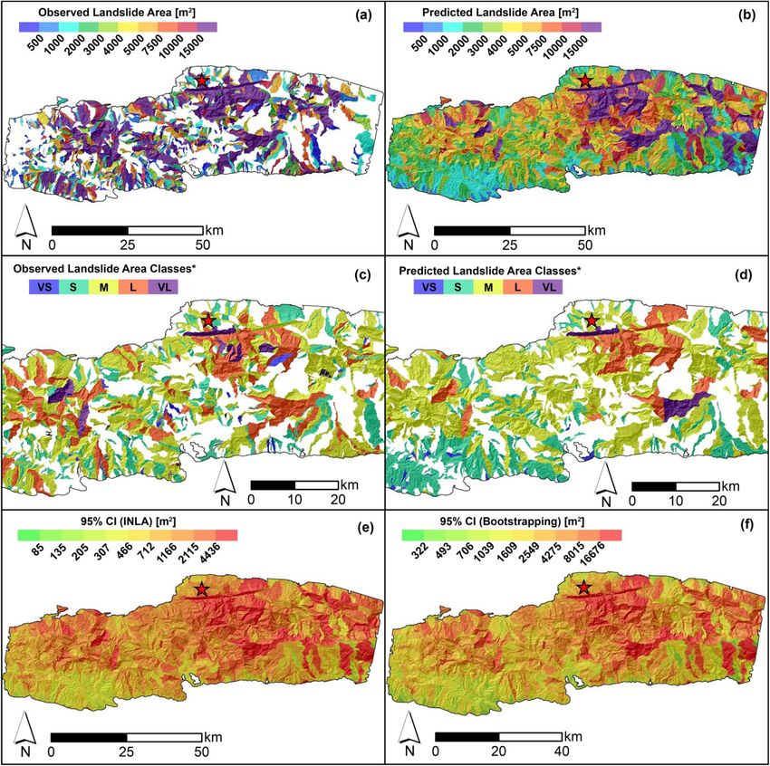
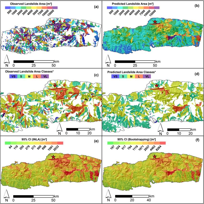
Here, we simulated 5000 predictive functions to estimate the mean In this section we present a summary of the model performance for
behaviour as well as the uncertainty in the landslide area prediction for each landslide size models, log(ALmax) and log(ALsum). We then provide
each SU. This is a crucial step because those SUs encompassing one or an overview of the inferred covariate effects and conclude presenting a
more landslides provide enough information to assess the whole spec­ graphical translation of the model's output into map form.
trum of possible landslide areas (mean and 95% CI for both the Max and
Sum models). However, the SUs where no landslides have been recorded
require the simulation step to recover analogous information. 5.1. Predictive performance

 Fig. 3 shows an overview of the model performance presented in
4.5. Goodness-of-fit and predictive performance assessment agreement with the three metrics we explored, namely, probability in­
 tegral transform (PIT) plots, observed vs. fitted values and coverage
 We here describe numerical and graphical methods to assess the probabilities. The top row shows the performance of the Max model,
goodness-of-fit and the predictive performance of our models. while the bottom row shows the performance of the Sum model. The
 collection of probabilities detailed in Section 4.5, computed using all the
 • Probability integral transform (PIT): PIT values are useful leave- training data, gives rise to the histogram in Fig. 3a,d. We can see that
 one-out goodness-of-fit measures. They are computed as follows both models capture the bulk of the distribution (bars close to the
 Pi = F− i (yi ), i ∈ {1, …, | |}, dashed line) reasonably well, but they do not seem to appropriately
 capture the tails of the landslide size distribution (bars far from the
 where F− i is the cumulative distribution of the i-th observation, yi, dashed line). The latter is expected since the normal and log-normal
 obtained from a model fitted using all the available data except yi, distributions have light tails, which implies that the model will give
 contains all the slope units s, and | | is the cardinality of , i.e., the fairly low probabilities (i.e., very close to 0) to extreme landslide sizes.
 number of slope units. A model with a perfect predictive ability We recall here that for a model to be optimal, the PIT plot should exhibit
 should have PIT values closely distributed according to a standard a uniform distribution. Here, we can see some moderate departure from
 uniform distribution. Indeed, assuming that F− i is continuous (which the uniform distribution in both cases, but this is expected for such a
 is the case here) the distribution of Pi, i = 1,…,| |, can be written as large dataset combining various heterogeneous EQIL inventories.
 Overall, the Max model seems to be better calibrated than the Sum
 Pr(Pi ≤ u) = Pr(F− i (yi ) ≤ u) = Pr(yi ≤ F−− i1 (u)), u ∈ (0, 1). model. Observed vs. fitted values look similar for both models (Fig. 3b,
 e), although the Max model exhibits pair of points slightly better aligned
 The model F− i has a perfect prediction ability if it is able to generate
 and equally spread along the 45◦ line. As for the coverage probabilities
 yi (the value that was left out). This means that F− i is a perfect pre­
 (Fig. 3c,f), both models appear to be surprisingly excellent with most of
 diction if yi ~ F− i which, in turns, implies that
 the nominal to sample coverage pairs very well aligned with the 45◦ line
 Pr(yi ≤ F−− i1 (u)) = F− i (F−− i1 (u))) = u. and the bulk of the distribution showing a negligible deviation from it.
 As mentioned in Section 4.5, the coverage plots are computed by
 The above equation implies that the distribution of the PIT values { simulating 5000 samples from each model and counting the proportion

 8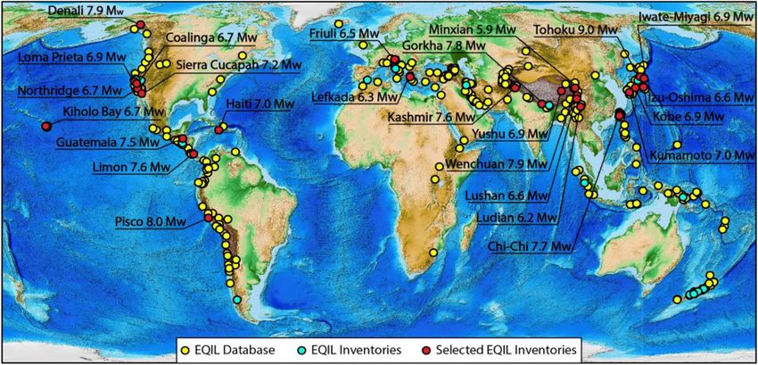

L. Lombardo et al. Engineering Geology 293 (2021) 106288

Fig. 3. Left to right: Probability integral transform (PIT) plots, fitted vs. observed plots (in log-scale), and coverage probabilities for the Max (top) and Sum (bot­
tom) models.

of times the observed data are within a (1− α)100 % simulated-based
credible interval, with α = {0.05, 0.10, …, 0.90} (the nominal
coverage). A model with a reasonable coverage should give a proportion
close to (1− α)100 %. We can see that our models succeed in recovering
the nominal coverage for extreme nominal coverage values, but they are
a bit off for central nominal coverage values. Overall, the Sum model
performs slightly better than the Max model.

5.2. Linear covariate effects

 Fig. 4 shows the estimated coefficients of linear (or fixed) effects
(except for the intercept) for the Max and Sum models. Notably, we plot
the 95% credible intervals originated from the Bootstrap rather than
directly from INLA, which incorrectly assumes conditional indepen­
dence for model fitting. We recall here that because of this, INLA may
largely underestimate the uncertainty compared to Bootstrap, which
more realistically accounts for spatial dependence at the data level. In
light of this, here we only report the Bootstrap uncertainty and do not
show the uncertainty directly estimated with INLA.
 The selected covariates, that have been rescaled to have mean 0 and
variance 1, show relatively strong positive and negative influences on
landslide sizes. More specifically, out of 17 covariates used linearly only
7 appeared to be significant for the Max model, and 8 for the Sum model.
Non-significance does not necessarily imply that the model is not
influenced by these covariates. Significance indicates that the model is Fig. 4. Posterior means (dots) of fixed linear effects (except the intercept) with
 Bootstrap-based 95% credible intervals (vertical segments) for the Max and
95% certain of the role (either positive or negative) of the given co­
 Sum models. The horizontal black dashed line indicates no contribution to the
variate with respect to the landslide size. Moreover, the extent to which
 landslide sizes.
a covariate—significant or not—contributes to the model is summarized
by the absolute value of the posterior mean regression coefficient.
 proxy for gravitational potential energy and by the MI, a proxy for the
 In this sense, the largest linear contributors for the Max model are MI
 ground motion stress. Intuitively, the easiest interpretation of the relief,
(avg) and Relief rng (avg), both with an absolute mean regression coef­
 is that from a SU with a larger relief or gravitational energy, one should
ficient of 0.50. Besides, Slope (std), VRM (avg), PRC (std) and Area SU
 expect larger landslides. However, this type of interpretation is difficult
contribute with absolute posterior mean coefficients of 0.42, 0.18, 0.16
 to be uniquely identified because the inventories mix up landslides of
and 0.13, respectively. From these ranks, the contribution becomes less
 different types without a distinction between failure and runout zones.
prominent and it decays down to the least contributor represented by MI
 The role of the slope steepness is also well represented in the model as
(std) with | ̂
 β| = 0.0007. The covariates appeared to be ranked with a well as the dimension of the mapping unit itself. Specifically, these
primary control on the estimated landslide size exerted by the relief, a

 9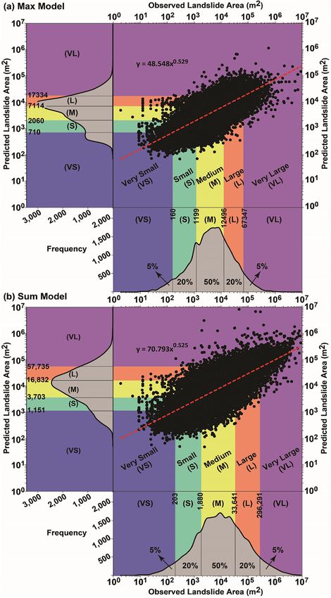

L. Lombardo et al. Engineering Geology 293 (2021) 106288

covariates present a significant and positive posterior distribution which complex and varying behavior. To interpret this panel, the regression
contributes to increase the expected landslide size (e.g., Medwedeff constants are site-specific indices of differences in landslide area
et al., 2020; Valagussa et al., 2019). Conversely, a negative regression response to the ground motion. In other words, with respect to the mean
coefficient, e.g., for VRM (avg), implies that larger landslide sizes for the landslide area across the whole dataset we used, the values reported
Max model are expected for smaller VRM (avg) values. The negative here lead to variations in landslide size typical of specific landscapes. For
contribution of the VRM (avg) is also consistent with the current liter­ instance, at a preliminary visual examination, the Gorkha earthquake
ature. For instance, Frattini and Crosta (2013) suggested that high clearly stands out with the smallest mean regression constant out of the
roughness implies a more dissected landscape with smaller sub-sectors 25 cases; the largest posterior mean is associated to the Guatemala
across a given slope unit. Thus, this setting could act as a limiting fac­ earthquake. Finally, few earthquakes inventories are aligned along the
tor for landslide size. zero line. In other words, they display no positive nor negative anomaly
 For the Sum model, the dominant fixed effect appears to be the MI with respect to the average landslide size of all 25 cases combined. More
(avg), with an absolute mean regression coefficient of 0.89. This is fol­ details and an extensive interpretation of these results will be provided
lowed by Relief rng (avg) with | ̂ β| = 0.68, Slope (std) with |̂ β| = 0.51, in Section 6.
VRM (avg) with |̂β| = 0.30, Area SU with | ̂
 β| = 0.23, Prof Cur (std) with A much simpler situation prevails for the Landforms (Fig. 5b). In fact,
 no landform class appears to be significant in our case and they all lay
| β| = 0.22 and VRM (std) with | ̂
 ̂ β| = 0.12.
 along the zero line, indicating a negligible effect onto the final model.
 We will discuss this in Section 6.
5.3. Non-linear covariate effects The Slope (avg) panel (Fig. 5c) shows a clear nonlinear behavior both
 in the Max and Sum models. SUs with an average steepness up to
 Fig. 5 displays all the non-linear (or random) covariates’ effects approximately 25 degrees do not contribute to vary the estimated
featured in our model, by plotting the estimated coefficients in terms of landslide size. From this threshold to larger steepness values, the Max
posterior mean and Bootstrap-based 95% credible intervals. Two panels model shows a mild increase in the Slope (avg) regression coefficients,
(top row and bottom left) report covariates that have been used in a whereas the Sum model also increases but with a much steeper trend.
purely categorical form, i.e., with class effects being mutually indepen­
dent a priori. The remaining panel (bottom right) shows the covariate
Slope (avg) being used as an ordinal variable with an adjacent inter-class 5.4. Landslide area classification
dependency driven by a random walk (see Section 4.1).
 The Earthquake Inventories multiple intercepts (Fig. 5a) show a We opt to translate the model results in map form following two

Fig. 5. Random effects for the Max and Sum models: earthquake inventories (top), landform classes (bottom left), and mean slope (Slp, bottom right). For the
earthquake inventories and landform classes, the dots show the posterior mean, while the segments correspond to the Bootstrap-based 95% credible intervals. For
mean slope, the curves show the posterior mean, while the shadowed polygons correspond to the Boostrap-based 95% credible intervals. In all the plots, the black
horizontal dashed line indicates zero (i.e., no contribution to the landslide sizes).

 10