Bat swarming as an inspiration for multi-agent systems: predation success, active sensing, and collision avoidance
←
→
Page content transcription
If your browser does not render page correctly, please read the page content below
Bat swarming as an inspiration for multi-agent systems:
  predation success, active sensing, and collision avoidance

                                       Yuan Lin

                      Dissertation submitted to the Faculty of the
                  Virginia Polytechnic Institute and State University
              in partial fulfillment of the requirements for the degree of

                                Doctor of Philosophy
                                         in
                               Engineering Mechanics

                              Nicole T. Abaid, Co-chair
                               Rolf Müller, Co-chair
                                     H. Pat Artis
                                  Mark S. Cramer
                                   Shane D. Ross

                                  February 1, 2016
                                 Blacksburg, Virginia

Keywords: Bat Swarming, Predation Success, Frequency Jamming, Collision Avoidance,
                                   Swarm Size
                            Copyright 2016, Yuan Lin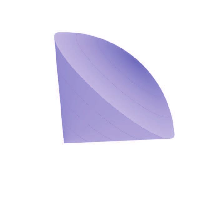
Bat swarming as an inspiration for multi-agent systems:
          predation success, active sensing, and collision avoidance

                                        Yuan Lin

                                        Abstract

Many species of bats primarily use echolocation, a type of active sensing wherein bats
emit ultrasonic pulses and listen to echoes, for guidance and navigation. Swarms of such
bats are a unique type of multi-agent systems that feature bats echolocation and flight
behaviors. In the work of this dissertation, we used bat swarming as an inspiration for
multi-agent systems to study various topics which include predation success, active sens-
ing, and collision avoidance. To investigate the predation success, we modeled a group of
bats hunting a number of collectively behaving prey. The modeling results demonstrated
the benefit of localized grouping of prey in avoiding predation by bats. In the topics re-
garding active sensing and collision avoidance, we studied individual behavior in swarms
as bats could potentially benefit from information sharing while suffering from frequency
jamming, i.e., bats having difficulty in distinguishing between self and peers informa-
tion. We conducted field experiments in a cave and found that individual bat increased
biosonar output as swarm size increased. The experimental finding indicated that individ-
ual bat acquired more sensory information in larger swarms even though there could be
frequency jamming risk. In a simulation wherein we modeled bats flying through a tunnel,
we showed the increasing collision risk in larger swarms for bats either sharing informa-
tion or flying independently. Thus, we hypothesized that individual bat increased pulse
emissions for more sensory information for collision avoidance while possibly taking ad-
vantage of information sharing and coping with frequency jamming during swarming.

The research is supported by the National Science Foundation [grant CMMI-1342176],
the National Natural Science Foundation of China [grant numbers 10774092 and 451069],
the Chinese Ministry of Education (Tese Grant), the Institute for Critical Technology and
Applied Science at Virginia Tech, and the Fundamental Research Fund of Shandong Uni-
versity [No. 2014QY008].
Acknowledgments
I would like to thank all the people who have been supportive to me pursuing my doctoral
degree at Virginia Tech. First of all, I would like to thank both my advisors, Drs. Abaid
and Müller, for their tremendous help during my research years. Dr. Abaid brought me
to the field of multi-agent systems and advised me to learn the method of agent-based
modeling. My MATLAB coding skill was also improved under her advisorship. Since I
joined Dr. Müller’s lab in Fall 2014, I obtained better knowledge in biosonar systems and
signal processing. Dr. Müller also offered me critical advice that improved my scientific
writing. I also wouldn’t forget that Dr. Müller gave me a hand when I had trouble in
graduate school.
The other three committee members were also helpful in my doctoral study in many as-
pects. I enjoyed my interactions with Dr. Artis, who was always helpful in me pursuing
my career. Dr. Artis gave me comments on my writing and offered me advice to help me
succeed. Dr. Cramer was helpful in me learning engineering mechanics courses, which
had me think about problems and issues from a totally different perspective. I enjoyed
taking the courses in dynamical systems and control by Dr. Ross. Dr. Ross explained
dynamics topics in very clear ways, which benefited me a lot in my logical thinking.
I was also grateful to having taken the robotics courses and worked with Dr. Kevin
Kochersberger on unmanned systems at Virginia Tech. I developed great interest in robotics
through the projects that I did on unmanned ground/aerial vehicles. Particularly, I had the
opportunity to work with Dr. Kochersberger on drone application in farming in his Un-
manned Systems Lab, where I saw the possibility of immediate use of university technol-
ogy in the real world.
There are so many people who encouraged me so much at whatever phases of my life.
My mother is always proud of me; my father loves me with few words; my sister shares
with me articles with deep societal and historical meanings. Jay and Michelle Lester and
other attendees from International Christian Fellowship offered so much positive thinking
iiithat turned me into a person with greater gratitude. My international group at New Life
Christian Fellowship helped me through the alone years in the United States. There were
so many friends (students, staff, and faculty) in the Engineering Mechanics program that
provided invaluable help for me to pass the program exams to graduate.
In addition, I was blessed to have worked with other fellow hokies to start the Aerial
Robotics Club (ARC) at Virginia Tech. The startup provided me opportunities to learn
to lead a team in the United States and pursue my career in robotics with the help from
multi-nationals. It was great to work with many amazing people from the club who are
doing amazing things that could possibly change people’s life.
Last but not least, I would like to express my gratitude to the Department of Biomedical
Engineering & Mechanics and the Department of Physics at Virginia Tech as they hired
me as a teaching assistant in the past years.
ivContents
1 Introduction 1
1.1 Multi-agent animal systems . . . . . . . . . . . . . . . . . . . . . . . . . 1
1.2 Bat swarms . . . . . . . . . . . . . . . . . . . . . . . . . . . . . . . . . 2
1.3 Research topics and attribution . . . . . . . . . . . . . . . . . . . . . . . 2
2 Bat predation success and prey collective behavior - simulation 4
2.1 Abstract . . . . . . . . . . . . . . . . . . . . . . . . . . . . . . . . . . . 4
2.2 Introduction . . . . . . . . . . . . . . . . . . . . . . . . . . . . . . . . . 5
2.3 Modeling . . . . . . . . . . . . . . . . . . . . . . . . . . . . . . . . . . 6
2.3.1 Model description . . . . . . . . . . . . . . . . . . . . . . . . . 6
2.3.2 Predator velocity update algorithm . . . . . . . . . . . . . . . . . 8
2.3.3 Prey velocity update algorithm . . . . . . . . . . . . . . . . . . . 9
2.4 Observables . . . . . . . . . . . . . . . . . . . . . . . . . . . . . . . . . 10
2.5 Simulation results . . . . . . . . . . . . . . . . . . . . . . . . . . . . . . 14
2.6 Discussion . . . . . . . . . . . . . . . . . . . . . . . . . . . . . . . . . . 19
3 Bat pulse emission and swarm size - field experiment 22
3.1 Abstract . . . . . . . . . . . . . . . . . . . . . . . . . . . . . . . . . . . 22
3.2 Introduction . . . . . . . . . . . . . . . . . . . . . . . . . . . . . . . . . 23
v3.3 Materials and methods . . . . . . . . . . . . . . . . . . . . . . . . . . . 24
3.3.1 Animals and location . . . . . . . . . . . . . . . . . . . . . . . . 24
3.3.2 Field experiment setup . . . . . . . . . . . . . . . . . . . . . . . 24
3.3.3 Data set . . . . . . . . . . . . . . . . . . . . . . . . . . . . . . . 26
3.3.4 Video processing . . . . . . . . . . . . . . . . . . . . . . . . . . 26
3.3.5 Audio processing . . . . . . . . . . . . . . . . . . . . . . . . . . 30
3.4 Results . . . . . . . . . . . . . . . . . . . . . . . . . . . . . . . . . . . . 30
3.5 Discussion . . . . . . . . . . . . . . . . . . . . . . . . . . . . . . . . . . 36
4 Bat pulse emission and swarm size - simulation 39
4.1 Abstract . . . . . . . . . . . . . . . . . . . . . . . . . . . . . . . . . . . 39
4.2 Introduction . . . . . . . . . . . . . . . . . . . . . . . . . . . . . . . . . 40
4.3 Modeling . . . . . . . . . . . . . . . . . . . . . . . . . . . . . . . . . . 41
4.3.1 Model description . . . . . . . . . . . . . . . . . . . . . . . . . 41
4.3.2 Position and velocity updates . . . . . . . . . . . . . . . . . . . . 44
4.4 Observables . . . . . . . . . . . . . . . . . . . . . . . . . . . . . . . . . 47
4.5 Simulation results . . . . . . . . . . . . . . . . . . . . . . . . . . . . . . 48
4.6 Discussion . . . . . . . . . . . . . . . . . . . . . . . . . . . . . . . . . . 52
5 Conclusions 57
5.1 Research summary . . . . . . . . . . . . . . . . . . . . . . . . . . . . . 57
5.2 Possible engineering applications . . . . . . . . . . . . . . . . . . . . . . 58
References 59
Appendix - Journal copyright permissions 72
viList of Figures
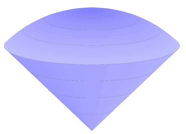
2.1 Schematic of three-dimensional sensing geometry for one predator (red
circle) and one prey (black circle). The predator i has position x̂i and
velocity v̂i ; the prey k has position xk and velocity vk . The blue cone
shows the predator’s sensing space with sensing range r̂s , angular range φ̂,
and eating range r̂e . The grey sphere shows the prey’s sensing space with
sensing range rs . . . . . . . . . . . . . . . . . . . . . . . . . . . . . . . 7
2.2 Frames of model simulation with 10 predators and 500 interacting prey
when (a) η = 0, (b) η = 0.2, and (c) η = 1. Red dots show predators’
positions which coincide with the apex of the blue spherical cones showing
their sensing spaces; black dots show prey’s positions. The unit for the
numbers on the axes is meter. . . . . . . . . . . . . . . . . . . . . . . . . 13
2.3 Mean ((a) and (d)) polarization, ((b) and (e)) cohesion, and ((c) and (f))
natural logarithm of cell occupancy parameter for interacting and inde-
pendent prey, respectively. Contour plots are displayed as prey population
size N and perturbation parameter η are varied. The black circles show
the mean observable values obtained from the model with independent
prey and the blue crosses show results of Monte Carlo simulations. The
superscript bar notation denotes the mean over the replicates and the er-
ror bars denote standard deviations over all selected values of η. Insets in
the second row show contour plots for independent prey. For each inset,
the color map is consistent with the contour plot above, that is, with the
corresponding observable for interacting prey. . . . . . . . . . . . . . . . 15
2.4 Mean prey cell coverage, as prey perturbation parameter η is varied. The
superscript bar notation denotes the mean over the 15 replicates and the
error bars denote standard deviations over all selected values of N. . . . . 16
vii2.5 Mean number of eaten (a) interacting and (b) independent prey, as prey
population size N and perturbation parameter η are varied. . . . . . . . . 17
3.1 Field experiment setup in the cave. (a) Schematic layout of the setup (lon-
gitudinal section) (b) Example gray-scale frame from the video recording
showing the setup. The bright spots are the infrared lights. Only the cam-
era that produced this video frame was used for recording the data ana-
lyzed here – image data from the other cameras seen in the picture was not
used for the present study. . . . . . . . . . . . . . . . . . . . . . . . . . 25
3.2 Bat identification. (a) and (b) Same part of two adjacent gray-scale frames
which include all detected bats. (c) Automated bat identification. The
black and white image was obtained by setting the brightness threshold on
the absolute values of the frame difference between (a) and (b), and then
eliminating the non-bat artifacts. Each white circle grouped the white re-
gions whose nearest distances were less than the distance threshold (short
white line at the bottom-right) and represented one bat. (d) Manual bat
identification in the scaled frame difference. The black circles represented
bats manually identified. . . . . . . . . . . . . . . . . . . . . . . . . . . 26
3.3 Comparison between automated (Nba ) and manual (Nbm ) counts of the
number of bats based on 2306 pairs of Nba and Nbm estimates obtained
from the same frame. Each triangular marker shows the mean of all Nba
values for the same value of Nbm . The error bars denote one standard de-
viation above and below the mean. The dashed line represents equality
between Nba and Nbm . The inset histograms shows the number of occur-
rences for the values of Nba (empty bars) and Nbm (filled bars). . . . . . . 28
3.4 Audio processing. (a) Spectrogram representation of a sample audio record-
ing. The horizontal line pair denotes the frequency band 49-99kHz for
the Eastern bent-wing bats. (b) Normalized filtered signal of the sam-
ple recording after matched filtering using the artificial pulse template in
Fig. 3.5. The wavy curve on top of the signal is the envelop. The dashed
horizontal line denotes the threshold for pulse selection. . . . . . . . . . . 29
viii3.5 Synthetic bat pulse design for the Eastern bent-wing bat pulses. (a) Time-
domain normalized signal of a recorded bat pulse. The pulse was pre-
filtered using a Butterworth high-pass filter with the cutoff frequency at
47 kHz. The plus markers were connected by a straight line, so were the
cross markers. The triangular markers were fitted using a quadratic func-
tion (r 2 > 0.99). (b) Spectrogram representation of the real bat pulse. The
white circles were fitted using the inverse of a quadratic function (black
curve, r 2 = 0.98). (c) Time-domain signal of the designed artificial bat
pulse. (d) Spectrogram representation of the designed artificial bat pulse. . 31
3.6 Average number of bats N̄ba over the time period used in the analysis.
There are 2306 data points in the plot for the selected recording period of
2306×60 frames. Inset: number of data points for each N̄ba . . . . . . . . . 32
3.7 Time history of normalized ultrasonic power and swarm pulse rate for the
analyzed audio recording. (a) The normalized ultrasonic power p. Inset:
histogram of normalized p. (b) The swarm pulse rate Np . Inset: histogram
of Np . . . . . . . . . . . . . . . . . . . . . . . . . . . . . . . . . . . . . 32
3.8 The relationship between ultrasound power and swarm pulse rate (number
of pulses). (a) the normalized ultrasound power p as a function of swarm
pulse rate Np for the selected recording. There are 2306 data points with
each representing a pair of normalized p and Np values obtained for the
same 60-frame period. Straight line: linear fit (r 2 = 0.85). (b) the normal-
ized ultrasound power pM as a function of the number of pulses NpM for
the Monte-Carlo simulation. A circle denotes the mean of 1000 simula-
tion values of normalized pM for the same NpM . The error bar denotes one
standard deviation above and below the mean. . . . . . . . . . . . . . . . 33
3.9 Bat pulse emission behavior for the Eastern bent-wing bat. (a) The swarm
pulse rate Np as a function of the average number of bats N̄ba . Each data
point represents a pair of Np and N̄ba values for the same 60-frame period.
Solid curve: mean of all Np values for the same N̄ba . Straight line: linear
fit (r 2 = 0.8). (b) The individual pulse rate np as a function of the average
number of bats N̄ba . Each data point represents a pair of np and N̄ba values
for the same 60-frame period. Solid curve: mean of all np values for the
same N̄ba . . . . . . . . . . . . . . . . . . . . . . . . . . . . . . . . . . . 34
ix3.10 Bat distribution (normalized by the image width) as a function of the au-
tomated count of the number of bats Nba . The filled square and circular
markers show the averages of the means and standard deviations, respec-
tively, of bat vertical locations for the same Nba . The triangular and cross
markers show the averages of the means and standard deviations, respec-
tively, of bat horizontal locations for the same Nba . The error bars denote
one standard deviation above and below the averages. The thicker and
thinner error bars are for bat vertical and horizontal locations, respectively.
The dashed line denotes the image height. . . . . . . . . . . . . . . . . . 35
4.1 Schematic of three-dimensional sensing space and repulsion zone for bat
i. The bat has position xi and velocity vi . The spherical cone shows the
bat’s sensing space with sensing range rs and angular range of sensing φ.
The gray sphere shows the bat’s repulsion zone with radius rr . . . . . . . 42
4.2 Flow chart that summarizes the decision making and behavior of a bat at
each time step. . . . . . . . . . . . . . . . . . . . . . . . . . . . . . . . 46
4.3 Example frame of N = 100 bats flying through the tunnel with p = 0.5
and ηd = 0. Red circles and black triangles show positions of bats emitting
pulses and ceasing emission, respectively. The units for the axes are meters. 49
4.4 Average collision rate c versus the number of bats N with varying ηd val-
ues for p = 0.5 and with the case of no eavesdropping. Error bars showing
one standard deviation over the ten replicates are plotted at every point,
but are occluded by point markers due to their very small magnitude in
almost all cases. . . . . . . . . . . . . . . . . . . . . . . . . . . . . . . . 52
4.5 (a) The average collision rate c with varying N and p for ηd = 0; (b)
the ratio between the average collision rate with ηd = 0 and the average
collision rate with no eavesdropping. Here, c′ denotes the average collision
rate for simulations with no eavesdropping, which has similar trends as in
(a) but with larger values. . . . . . . . . . . . . . . . . . . . . . . . . . . 54
4.6 (a) The collision/jamming cost s1 and (b) the collision/energy cost s2 with
varying N and p for ηd = 0. In (a), the red curve denotes the minimum
collision/jamming cost for different N; the red dotted curve shows the
pulse emission rates corresponding to a constant collision/jamming cost
log10 (s1 ) = −2.8 for N ≤ 6. In (b), the blue curve denotes the minimum
collision/energy cost for different N. . . . . . . . . . . . . . . . . . . . . 55
xList of Tables
2.1 Parameter values for predators and prey. . . . . . . . . . . . . . . . . . . 12
4.1 Parameter values used in the simulation study. . . . . . . . . . . . . . . . 48
4.2 Simulation replicate length. . . . . . . . . . . . . . . . . . . . . . . . . . 49
xiChapter 1
Introduction
1.1 Multi-agent animal systems
Multi-agent systems are known as systems that include multiple autonomous agents in
a environment [1]. Multi-agent systems are observed in various settings such as robotic
teams [2, 3], computer networks [4], economic systems [5], and animal groups [6]. To our
interest, we study multi-agent systems of animal groups, i.e., multi-agent animal systems,
by taking animal swarming as an inspiration for multi-agent systems of broader sense.
Multi-agent animal systems usually involve interacting animals swarming in groups which
can be characterized as collective behavior. Animals across different species show collec-
tive grouping, such as schooling fish [7], flocking birds [8], lane-forming ants [9], and
column-forming bats [10]. It has been demonstrated that appropriate interaction rules
among agents lead to collective formation (coherent moving direction and relatively close
distance) [11]. The possible interaction rules may include alignment of velocity directions,
attraction to peers’ locations, and repulsion from peers that may cause collisions [12, 13].
While multi-agent swarming emerge due to the local interacting rules, the collective swarm-
ing also affects individual behavior reversely. The reverse relationship is characterized as
group-size effect wherein swarm size correlates with individual behavioral change. For ex-
amples, individual bird vigilance reduces in larger groups due to collective detection and
lower individual predation risk [14, 15]; wasp behavior is less complex in larger swarms
for completing fewer tasks [16]; dairy cattle’s food intake varies with group size because
of feeding competition and social comfort [17]. These examples indicate that swarming
results in both benefits and disadvantages for which animals modify individual behavior
1Yuan Lin Chapter 1 Introduction 2 to accommodate. 1.2 Bat swarms Bat swarms are unique multi-agent animal systems due to the nature of bat echolocation. Echolocation is defined as bats emit ultrasonic pulses and listen to the reflected echoes for guidance and navigation [18, 19]. Thus, echolocation is a kind of active sensing [20, 21, 22] which is different from passive sensing wherein agents do not emit self signals but instead use only existing environmental information for sensing. Bats’ acting sensing may post both constructive and destructive influences to individuals when bats form swarms. The influence is constructive if a bat possibly utilizes peers’ sensory information/listen to peers’ echoes for navigation, which is shown as bats’ eavesdropping behavior [23, 24]. This is also known as information sharing in engineering systems [25]. On the other hand, the influence is destructive if a bat cannot distinguish self and peers’ echoes for accurate navigation. This destructive influence is characterized as frequency jamming problem in bat groups [26, 27, 28]. To unveil bats’ behavior in maximizing the constructive influence while minimizing the destructive influence during collision-free swarming is one of the research goals in this dissection, as the findings could potentially inspire novel control algorithms for next-generation unmanned aerial vehicles with decentralized control [2, 3]. 1.3 Research topics and attribution The research in the dissertation is focused on bat swarming while covering various top- ics which include hunting success, active sensing, and collision avoidance. The papers documenting the research results have been published in or will be submitted to various journals and are shown in the following chapters. Specifically, for the topic of hunting success, we investigated the impact of prey collective formation extent on the predation success of a group of independent bats. We used the method of agent-based modelling and illustrated our findings through simulation results. Our results could potentially provide insights on the strategies for predation avoidance in multi-agent systems. The paper for this work (Chapter 2) has been published in the journal of Physical Review E [29]. A conference paper that documented the early stage of the results was published in the 2013 ASME Dynamics and Control Conference [30]. For the topics of active sensing and collision avoidance, we quantified the relationship be-
Yuan Lin                             Chapter 1 Introduction                            3

tween individual biosonar output and swarm size through field experiments. The research
was conducted in a cave wherein we recorded bat swarms using a camera and an ultrasonic
recorder. The results could help us understand the individual bat behavior for frequency
jamming avoidance through a global finding. The paper for this work (Chapter 3) will be
submitted to a journal [31].
At last, we studied the benefit of changing individual biosonar output with swarm size in
a multi-agent system through simulation. We allowed bats to utilize peers’ information in
the model. The benefit was quantified as collision avoidance success as collision is one
of the major concerns of real flights. This work could explain the findings through field
experiments in Chapter 3. The paper for this work (Chapter 4) has been published in the
Journal of Theoretical Biology [32]. A conference paper that documented the early stage
of the results was published in the 2014 ASME Dynamics and Control Conference [33].
Chapter 2

Bat predation success and prey
collective behavior - simulation

This chapter has been published in Physical Review E with the title “Collective behavior
and predation success in a predator-prey model inspired by hunting bats” [29].

2.1 Abstract
We establish an agent-based model to study the impact of prey behavior on the hunting
success of predators. The predators and prey are modeled as self-propelled particles mov-
ing in a three-dimensional domain and subject to specific sensing abilities and behavioral
rules inspired by bat hunting. The predators randomly search for prey. The prey either
align velocity directions with peers, defined as “interacting” prey, or swarm “indepen-
dently” of peer presence; both types of prey are subject to additive noise. In a simulation
study, we find that interacting prey using low noise have the maximum predation avoid-
ance because they form localized large groups, while they suffer high predation as noise
increases due to the formation of broadly dispersed small groups. Independent prey, that
are likely to be uniformly distributed in the domain, have higher predation risk under a
low noise regime as they traverse larger spatial extents. These effects are enhanced in
large prey populations, which exhibit more ordered collective behavior or more uniform
spatial distribution as they are interacting or independent, respectively.

                                            4
Yuan Lin Chapter 2 Bat predation success and prey collective behavior - simulation 5 2.2 Introduction Collective behavior is a striking phenomenon observed in animals of diverse species, like fish swimming in schools [7], birds flying in flocks [8], ants forming organized lanes [9], and mosquitoes flying in swarms [34]. This social behavior is known to provide a variety of benefits for individuals. For example, it may increase the chance for animals to locate food sources [35], conserve heat and energy of a colony [36], help an individual find a mate [37], and reduce the risk of being predated [38]. The benefit of protection from predation, which is of primary interest in this paper, results from the “many eyes” effect [15] and cognitive fusion to predators [39] when animals swarm in groups. The “many eyes” effect enables individuals to have better predator detection through information sharing with peers. An individual’s risk of being attacked is diluted by the presence of other group members, which may coalesce into a superorganism in the predator’s perception. Capturing the dynamics of such groups is of interest to a variety of scientific and engi- neering research questions. In the literature, collective behavior is modeled either through continuum approaches or by establishing agent-based models. For one type of contin- uum approach, the Navier-Stokes equations are applied to study collective behavior as the motion of a fluid [40, 41]; for another continuum-type approach, equations are derived using self-propulsion and velocity reorientation of particles obeying a discrete model [42]. In addition to these modeling efforts, extensive research has been devoted to developing agent-based models, wherein individuals are considered as dynamic particles interacting with peers homogeneously [43]. The agent’s behavioral responses are defined using dis- crete decision making [44, 45] or by building potential functions based on the state of the group [46, 47, 48]. Among models defining a decision making process, common rules applied to individuals for interacting with peers include “repulsion”, “alignment”, and “at- traction”. The “repulsion” rule mandates that each individual keeps a certain distance from peers; the “alignment” and “attraction” rules dictate that group members seek consensus in orientations and positions, respectively. Typical models based on such rules and potential functions generate collective behavior [12, 13, 49, 34] as group-level structures emerge from established principles of behavioral algorithms prescribed to individuals [11]. Research using agent-based models has also tackled the predator-prey relationship; such work finds that the relative population sizes, as well as overall species fitness, can be re- fined by varying model parameters. In [50], the ranges of sensing for predators and prey are varied to explore a model with carnivorous predators, herbivorous prey, and plants sub- ject to behavioral rules. The authors find that increasing the sensing range for predators is beneficial for individual survival and detrimental for predator population size; analogously, increasing prey sensing range results in a smaller prey population. The steady-state pop-
Yuan Lin    Chapter 2 Bat predation success and prey collective behavior - simulation        6

ulation dynamics of predators and prey are investigated in [51], which finds that agents’
initial conditions and the spatial arrangement and availability of resources for prey, such as
food and refuge, determine the distribution of system behaviors. We comment that these
studies only consider agents moving in discrete two-dimensional domains.
In this paper, we establish an agent-based predator-prey model in a three-dimensional do-
main to explore the relationship between the collective behavior of prey and predation
success. The agents, predators and prey, are modeled as self-propelled particles inspired
by rules common to the animal kingdom, that is, both predators and prey sense the environ-
ment, and predators hunt for and feed on prey. In the model, the sensing mechanisms and
behavioral rules implemented in predators and prey represent the biological system of in-
sectivorous bats and the insects they hunt [52, 53, 54]. In particular, predators are equipped
with a limited sensing space that is analogous to bats’ sonar beam pattern [55, 56], which
is a key factor in determining their hunting success, and the prey are not capable of sensing
the predators. We consider two cases in terms of prey’s behavior: i) prey exhibit collective
behavior à la Vicsek [57] by orienting velocity directions with peers subject to additive
noise, and ii) prey swarm independently as random walkers subject to noise. By compar-
ing simulation results of the two prey-swarming cases, we find that, in a sufficiently large
environment, prey forming a few localized cohesive groups have a low chance of being
detected by predators. Conversely, if prey are uniformly positioned in the environment,
limited rather than extensive traversal of the domain is a better strategy to avoid predation.
These results validate the current views held in the biological community that protection
from predation is a significant motivator of collective behavior.

2.3 Modeling

2.3.1 Model description

We consider a system of N̂ + N agents moving in a cube of side length L with periodic
boundary conditions in discrete time. In the three-dimensional domain, the agents are
partitioned into N̂ predators and N prey with constant velocity magnitudes ŝ and s, re-
spectively. Each predator has a three-dimensional sensing space, a spherical cone. For the
spherical cone, its apex is the predator’s position; its side length is the predator’s sensing
range r̂s ; and its opening angle is the predator’s angular range of sensing φ̂. The predator’s
velocity vector starts at the apex of the spherical cone and aligns with its central axis. For
Yuan Lin Chapter 2 Bat predation success and prey collective behavior - simulation 7
predator i, i = 1, 2, . . . , N̂, the position update at time t + ∆t is
x̂i (t + ∆t) = x̂i (t) + v̂i (t + ∆t) ∆t (2.1)
where t, ∆t ∈ R+ , ∆t is a constant, and x̂i , v̂i ∈ R3 are the predator’s position and
velocity vectors, respectively.
Each prey has a spherical sensing space whose center is the prey’s position and whose
radius equals the prey’s sensing range rs . At time t, the position vector of prey k, k =
1, 2, . . . , N, is xk (t) ∈ R3 and its velocity vector is vk (t) ∈ R3 . The position update for
prey is the same as above for predators in (2.1). A schematic of the model geometry is
shown in Figure 2.1.
ෝ
࢜
߶
ෝ
࢞
࢜
࢞
ݎ௦
Figure 2.1: Schematic of three-dimensional sensing geometry for one predator (red circle)
and one prey (black circle). The predator i has position x̂i and velocity v̂i ; the prey k
has position xk and velocity vk . The blue cone shows the predator’s sensing space with
sensing range r̂s , angular range φ̂, and eating range r̂e . The grey sphere shows the prey’s
sensing space with sensing range rs .
The initial positions and velocity directions of predators and prey in R3 are generated
with uniformly distributed random probability in the cube of side length L centered at
the coordinate origin and in the unit sphere [58], respectively. The state update for both
predators and prey depends only on the preceding time step. In the following, we define
algorithms to update the velocity directions of predators and prey.Yuan Lin Chapter 2 Bat predation success and prey collective behavior - simulation 8
2.3.2 Predator velocity update algorithm
In the model, predators are designed to randomly search in the domain until they detect
prey, after which they head towards the nearest prey detected. Thus, we define the fol-
lowing two rules to update the velocity directions for predators: a predator heads towards
(“hunts”) prey if prey are detected and walks randomly if prey are not detected.
The hunting rule mandates that predators head towards prey that occupy their sensing
spaces. When a predator’s sensing space is occupied by at least one prey, the predator
chooses the nearest prey as a target and orients its velocity direction towards it persistently
until the prey is no longer in the sensing space, which is similar to hunting in big brown
bats [59]. If the distance between the predator and the prey is less than the eating range r̂e
in the sensing space, the prey is considered to be “eaten”. In this case, the prey’s position
and velocity vectors are randomly reassigned with uniform distribution at the next time
step, which results in a prey population of fixed size. When the hunted prey is eaten,
the predator chooses the next closest prey in its sensing space and keeps on hunting. We
comment that prey that are isolated are not preferentially selected as targets of predators,
since the periodic boundary conditions constrain the prey population by design. We define
the set of prey that occupy predator i’s sensing space at time t as Ni (t) and the index of
the prey targeted as k ∗ . Then the hunting velocity update for the predator is
xk∗ (t) − x̂i (t)
v̂ih (t + ∆t) = ŝ , k ∗ ∈ Ni (t) (2.2)
kxk∗ (t) − x̂i (t)k
If there are no prey in a predator’s sensing space, the predator behaves as an independent
random walker. In this case, a predator’s velocity direction relies only on its previous
velocity perturbed by a random noise defined by a perturbation parameter η̂. The random-
walking velocity update for the predator is
v̂i (t) + ω(η̂)
v̂iw (t + ∆t) = ŝ (2.3)
kv̂i (t) + ω(η̂)k
where ω(η̂) ∈ R3 is a realization of a vector-valued random variable whose magnitude
is given by a Gaussian distribution with mean zero and standard deviation ŝ tan(η̂π) and
whose direction is uniformly distributed in the plane that is normal to the predator’s veloc-
ity direction at time t. The magnitude of ω(η̂) is restricted to the interval [0, ŝ tan(η̂π)],
which enforces the angle between v̂iw (t + ∆t) and v̂i (t) is less than or equal to η̂π. When
η̂ = 0, the angle between these two vectors is always zero; when η̂ = 1, this angle varies
between zero and π. Loosely speaking, larger values of η̂ result in higher random noise
added at each time step, and thus, more convoluted trajectories for the predators. To avoidYuan Lin Chapter 2 Bat predation success and prey collective behavior - simulation 9
unrealistically large values of this noise, which may occur since the Gaussian distribution
is defined in R, the realization of the random variable is regenerated when its magnitude
has a value outside the stated interval. This restriction also ensures that the normalization
with respect to the random noise term is defined.
We update the predator’s velocity using the hunting and random-walking updates as
(
v̂ih (t + ∆t), for Ni (t) 6= ∅
v̂i (t + ∆t) =
v̂iw (t + ∆t), else
We note that predators in the model do not interact with their peers, which is selected to
agree with observations on groups of bats that congregate socially but do not move or hunt
as a typical collective [60].
2.3.3 Prey velocity update algorithm
Based on whether or not prey interact with each other, we define two types of prey behavior
to update their velocity directions: interacting prey align velocity directions with peers
with Gaussian-distributed random noise and independent prey swarm randomly in addition
to noise.
The alignment ability is defined for interacting prey in three dimensions based on Vicsek’s
model [61]. If the distance between a prey’s position and its peer’s position is less than the
prey’s sensing range rs , the peer occupies the prey’s sensing space. We denote Nk (t) as
the set of indices of prey that occupy prey k’s sensing space at time t, with k ∈ Nk (t) by
convention. Prey k’s provisional velocity update, uk (t + ∆t), is given by the average of
the velocity vectors of prey l ∈ Nk (t). In other words,
P
l∈N (t) vl (t)
uk (t + ∆t) = s P k (2.4)
k l∈Nk (t) vl (t)k
The provisional velocity update is perturbed by Gaussian-distributed random noise defined
by a perturbation parameter η, which is analogous to random walking for predators defined
above. Therefore, we obtain the velocity update for prey k as
uk (t + ∆t) + ω(η)
vk (t + ∆t) = s (2.5)
kuk (t + ∆t) + ω(η)k
Independent prey swarm randomly using a rule analogous to the random walking velocity
update in predators [62]. However, independent prey use the noise parameter η similarlyYuan Lin Chapter 2 Bat predation success and prey collective behavior - simulation 10
to interacting prey. The two types of prey behavior can be achieved by using rs 6= 0 for
interacting prey and rs = 0 for independent prey. In other words,
uk (t + ∆t) = vk (t) (2.6)
for independent prey, since interactions with peers are not considered. With the maximum
noise at η = 1, interactions among prey are totally dominated by noise and both interacting
and independent prey exhibit the same random swarming behavior. We note that, although
we define interactions among prey based on metric distances in line with [57, 61], similar
collective behavior also results from prey interacting with peers selected using topological
distances [7, 8], which may be implemented analogously.
We comment that prey’s velocity update is not influenced by predators’ behavior because
prey do not detect predators in the model. As a result, there is no self-protection in prey
from being predated upon. This assumption is in accordance with examples of insectivo-
rous bats’ prey, such as flying beetles, which do not evade hunting bats [63]. Moreover,
lack of bi-directional perception between predators and prey necessitates the selection of
only a single time scale for the decision making process, which is based on the predators
alone since their hunting success is the variable of interest.
2.4 Observables
We define four observables to evaluate the behavior of prey: polarization, cohesion, cell
occupancy parameter, and cell coverage. The polarization measures the alignment of prey;
the cohesion captures prey grouping; the cell occupancy parameter conveys the spatial
distribution of prey grouping; and the cell coverage shows the extent covered by an average
prey trajectory. Note that high polarization, cohesion, and cell occupancy parameter values
indicate prey collective behavior for moderate or large prey population sizes. Finally, the
predation success is quantified as the average number of prey eaten by each predator per
time step.
The polarization of prey is calculated as the absolute value of their average normalized
velocities [57]. In other words, the prey polarization at time t is
N
1 X vk (t)
p(t) = (2.7)
N k=1 s
The value of p(t) ranges from 0 to 1, where 0 means that prey velocity directions are
homogeneously oriented in the unit sphere and 1 means that all prey are moving in the
same direction. Note that, the polarization is 1 for the number of prey N = 1.Yuan Lin Chapter 2 Bat predation success and prey collective behavior - simulation 11
We compute the prey cohesion based on the method of average nearest neighbor [64],
which allows equally high values when prey form large or small groups. In particular, the
cohesion is given by the average distance between prey and their nearest peers [65]. With
a reference distance Ld , the prey cohesion at time t is
N
!
1 X
c(t) = exp − dk (t) (2.8)
NLd
k=1
where
dk (t) = min kxl (t) − xk (t)k, l = 1, 2, . . . , N (2.9)
l6=k
is the distance between prey k and its nearest peer at time t. The reference distance Ld is
defined as the cut-off length between peers that are nominally near and far and thus can be
used to tailor the absolute magnitude of cohesion. The cohesion c(t) varies between 0 and
1, where a large value indicates high cohesion.
To obtain the cell occupancy parameter and cell coverage, we divide the cubic domain into
cubic cells with equal side length Lc . We select Lc as a factor of L so that the number of
cells is (L/Lc )3 , which is an integer. The number of prey in cell m, denoted as no (m, t),
divided by the total number of prey N is the normalized cell occupancy o(m, t) of the cell
at time t. In other words,
no (m, t)
o(m, t) = (2.10)
N
The normalized cell occupancies of all the cells are sorted by magnitude from greatest to
least to obtain the normalized sorted cell occupancy at time t, which quantifies the extent
of prey groups similarly to the density profiles considered in [66]. The distribution of
the normalized sorted cell occupancy which shows large occupancy values for a small
number of cells indicates that prey form a small number of large groups. On the contrary,
flatter distributions show that prey individuals are likely to be uniformly distributed in
the domain. Since most distributions exhibit approximately exponential decay based on
inspection, we average the normalized sorted cell occupancy with respect to time for the
simulation and fit it with an exponential probability density function [67], which is
f (y, λ) = λe−λy (2.11)
where y is the index of the average sorted cell occupancy for each cell, which is a positive
integer between one and the total number of cells, f is the average normalized sorted cell
occupancy, and λ is the cell occupancy parameter obtained by fitting the above distribution.
The value of λ is larger for distributions which are peaked for a small number of cells andYuan Lin Chapter 2 Bat predation success and prey collective behavior - simulation 12
Table 2.1: Parameter values for predators and prey.
Predators Prey
Parameter Symbol Value Symbol Value Unit
Population size N̂ 10 N 5 - 1000 -
Speed ŝ 0.5 s 0.25 m/∆t
5 2.5 m/s
Sensing range r̂s 5 rs 2.5 m
Perturbation parameter η̂ 0.1 η 0-1 -
Time interval for cell coverage - - ∆τ 150 ∆t
◦
Angular range of sensing φ̂ 120 - -
Eating range r̂e 0.5 - - m
Reference distance for cohesion - - Ld 5 m
exhibit fast decay, and it is smaller for distributions which are approximately constant and
exhibit slow decay.
The discrete spatial cells are also used to measure the straightness of prey’ paths. We define
the cell coverage for prey k, denoted as nc (k, t), to be the number of distinct cells that the
prey’s trajectory occupies during the time interval [t, t + ∆τ ] for a constant ∆τ ∈ R+ .
Cell coverage with a value of one means that the prey resides in the same cell with a
convoluted trajectory over the time interval, while a higher cell coverage value means that
the prey traverses a large extent of the domain by moving over a fairly straight path. Note
that, when computing the cell coverage for prey, we neglect time intervals in which prey
are eaten because their positions are regenerated randomly in the domain which results in
discontinuous prey trajectories.
The average number of prey eaten by each predator per time step is obtained to evaluate
predation success during simulation. This quantity is calculated as
Ne
n̄e = (2.12)
N̂T
where Ne denotes the total number of prey eaten over the entire simulation length in time
steps, defined as T . We comment that this metric is normalized by the number of predators
to highlight their ability to hunt in the environment of variable resources and is thus not
normalized by the number of prey present.Yuan Lin Chapter 2 Bat predation success and prey collective behavior - simulation 13
20
0
−20
20
20
0
0
−20 −20
(a)
20
0
−20
20
20
0
0
−20 −20
(b)
20
0
−20
20
20
0
0
−20 −20
(c)
Figure 2.2: Frames of model simulation with 10 predators and 500 interacting prey when
(a) η = 0, (b) η = 0.2, and (c) η = 1. Red dots show predators’ positions which coincide
with the apex of the blue spherical cones showing their sensing spaces; black dots show
prey’s positions. The unit for the numbers on the axes is meter.Yuan Lin Chapter 2 Bat predation success and prey collective behavior - simulation 14 2.5 Simulation results We seek to determine the parameters of the model for the simulation study by taking inspi- ration from biological systems. The predators’ sensing range is taken as r̂s = 5m and their angular range of sensing is φ̂ = 120◦ , which are physical parameters from big brown bats, Eptesicus fuscus [59, 68]. The prey’s sensing range is taken as half that of the predators’, which is rs = 2.5m. The predator speed is taken as the bat nominal flying speed 5m/s [69] and the same proportionality between predator and prey sensing ranges is assumed for their velocities. With the prey velocity smaller than the predators’, the predators are likely to achieve predation once they sense prey. We consider the population size of predators as N̂ = 10 and the side length of the domain as L = 50m, such that the density of predators is 0.08 per 1000m3 . The low density of predators in the domain ensures sufficiently large space for each predator to hunt and lowers their chance of collisions that are neglected in the model, consistently with collision avoidance in bats’ behavior [54]. The perturbation parameter for the predator swarm is η̂ = 0.1, which results in relatively straight trajectories which may occur in bats’ flights [70, 71]. We take the eating range r̂e as the distance a predator travels in one time step which is defined as ∆t = 0.1s for all simulations. In computing prey cohesion, we take the cut- off length Ld = 5m equal to the diameter of the prey spherical sensing space, which is the threshold above which two prey are not able to interact directly or indirectly through common neighbors. By this definition, two prey separated by Ld have a cohesion of 1/e = 0.368, which defines a nominally small value for this observable. For the simulation study, we consider the hunting behavior of predators with various prey population sizes ranging from 5 to 1000. Thus, the density of prey varies from 0.04 per 1000m3 to 8 per 1000m3 . The side length of the cubic cells is taken as Lc = 10m, such that the volume of one cell is 1000m3 and the total number of cells in the domain is 125. The time interval for prey cell coverage, ∆τ is taken as 150 ∆t, which gives 37.5m if a prey travels straight with velocity of 0.25m/∆t. This selected time interval ensures that a prey can potentially traverse multiple cells, while eliminating double counting a periodic trajectory since the maximum distance that a prey travels is less than L. For both cases of interacting prey and independent prey, the prey perturbation parameter η varies from 0 to 1, which enables us to obtain both the minimum and maximum effects from random noise. Table 2.1 gives a summary of the parameter values used in the simulation study. Figure 2.2 shows exemplary frames of predators and interacting prey swarming in simu- lations with N = 500. We see that, with η = 0, interacting prey form relatively large groups, while with η = 0.2, they form small groups comprising a few nearby peers. When η = 1, interacting prey are likely to be homogeneously positioned in the domain with
Yuan Lin Chapter 2 Bat predation success and prey collective behavior - simulation 15
p̄ c̄
1 1 1 0.8
0.3
0.4
0.1
0.5
0.8 0.8 0.8
0.6
0.6 0.6 0.6
0.6
0.3
0.4
0.1
0.5
0.4
η
η
0.4 0.1 0.4 0.4
0.6
0.1 0.2
0.2 0.2 0.2
0.1 0.5 0.5
0.3
0.7
0.4
0.5 0.6
0.5 0.9
0 0 0 0
0 250 500 750 1000 0 250 500 750 1000
N N
(a) (b)
ln(λ̄) 0.8
Independent − model
1 −1 Independent − Monte Carlo
−4
0.6
−3
0.8 1
−2
−3.5
0.6 0.5
η
0.4
p̄
−4
η
−4 −3
−3
0.4
0
500 1000
−3.5
0.2 N
0.2 −3.5 −3.5
−4
−3 −3 −3
0 0
0 250 500 750 1000 0 250 500 750 1000
N N
(c) (d)
0.8 0
Independent − model Independent − model
Independent − Monte Carlo Independent − Monte Carlo
0.6 −1
1
ln(λ̄)
1 −2 0.5
η
0.4
c̄
0.5
η
−3 0
0.2 500 1000
N
0
500 1000 −4
N
0
0 250 500 750 1000 0 250 500 750 1000
N N
(e) (f)
Figure 2.3: Mean ((a) and (d)) polarization, ((b) and (e)) cohesion, and ((c) and (f)) natural
logarithm of cell occupancy parameter for interacting and independent prey, respectively.
Contour plots are displayed as prey population size N and perturbation parameter η are
varied. The black circles show the mean observable values obtained from the model with
independent prey and the blue crosses show results of Monte Carlo simulations. The
superscript bar notation denotes the mean over the replicates and the error bars denote
standard deviations over all selected values of η. Insets in the second row show contour
plots for independent prey. For each inset, the color map is consistent with the contour
plot above, that is, with the corresponding observable for interacting prey.Yuan Lin Chapter 2 Bat predation success and prey collective behavior - simulation 16
no observable clusters. Thus, the three representative values of η - 0, 0.2, and 1 - are
considered to be associated with low, moderate and high noise for prey, respectively. For
simulations with independent prey, the distributions of particles in the domain are similar
to Figure 2.2(c). In addition, the motion of each agent follows a straighter trajectory as the
noise is decreased.
For the simulation study, we take T = 25 000 time steps as one simulation replicate and
average the prey’s polarization, cohesion, normalized sorted cell occupancy, cell coverage,
and the predator’s predation success within each replicate with respect to time. Moreover,
the cell occupancy parameter λ for each replicate is obtained by fitting the average nor-
malized sorted cell occupancy to the exponential probability density function; the cell
coverage values are obtained for each replicate by partitioning the time series into time
intervals of length ∆τ . Simulations are recorded after excluding an initial transient phase
of 10 000 time steps. Fifteen replicates are considered for each set of parameters. The
number of replicates and the simulation length are selected to ensure stationarity of the
results. In other words, the mean of the averages for the observables over the 15 replicates
divided by their standard deviation is less than 10%.
7
Interacting prey
Independent prey
6
5
n̄c
4
3
2
0 0.5 1
η
(a)
Figure 2.4: Mean prey cell coverage, as prey perturbation parameter η is varied. The
superscript bar notation denotes the mean over the 15 replicates and the error bars denote
standard deviations over all selected values of N.
Through observation, we find that the mean polarization, cohesion, and cell occupancy pa-
rameter λ values remain practically constant for independent prey of fixed population size
as noise is varied; this result is absent for interacting prey. Thus, we report the polariza-Yuan Lin Chapter 2 Bat predation success and prey collective behavior - simulation 17
tion, cohesion, and cell occupancy parameter values for interacting prey in contour plots
as the number of prey N and the prey perturbation parameter η are varied in Figure 2.3(a),
Figure 2.3(b), and Figure 2.3(c), respectively. These quantities are shown for independent
prey in plots with varying N only, see the black dashed curves in Figure 2.3(d), Fig-
ure 2.3(e), and Figure 2.3(f); insets inside these three plots display the contour plots which
show vertical striation characteristic of the observables. We comment that many contours
do not appear smooth due to the small number of data points for large prey population
sizes and the lack of smoothing the raw data.
n̄e n̄e
1 0.08 1 0.08
0.03
0.05
0.01
0.01
0.05
0.03
0.8 0.8
0.07 0.06 0.06
0.6 0.6
0.05
0.03
0.01
0.01
0.04 0.04
0.07
0.05
η
η
0.03
0.4 0.4
0.0 0.02 0.02
0.2 7 0.2
0.05
0.03
0.05
0.07
0.01
0.01
0.0 0.05
0 3 0 0 0
0 250 500 750 1000 0 250 500 750 1000
N N
(a) (b)
Figure 2.5: Mean number of eaten (a) interacting and (b) independent prey, as prey popu-
lation size N and perturbation parameter η are varied.
The polarization, cohesion, and cell occupancy parameter values of independent prey are
verified through a Monte Carlo simulation. We comment that the expected value for po-
larization may be computed analytically as a function of N in terms of random variables
defining uniformly distributed points on the unit sphere [58]. However, this procedure
requires evaluating 2N nested integrals, which poses both analytical and numerical chal-
lenges. Due to the nearest neighbor selection process inherent in the cohesion computation
and the sorting of cell occupancies, the cohesion and cell occupancy parameter may not be
analytically defined in integral expressions. Thus the Monte Carlo simulation is selected
for comparison of these observables to the model simulation. In the Monte Carlo simula-
tion, the particles are assigned with random velocity directions and positions at each time
step, thus omitting the dynamics of the model. The Monte Carlo simulations are com-
puted with 10 replicates analogously to the model simulations; observable values are also
obtained in the same way as above. The quantities from the Monte Carlo simulation are
denoted as blue crosses in the plots for independent prey.Yuan Lin Chapter 2 Bat predation success and prey collective behavior - simulation 18
In Figure 2.3(a), we see that the addition of noise is destructive to the polarization of
interacting prey. When the noise is low, interacting prey are highly polarized. However,
when the noise increases to the moderate level at η = 0.2, the polarization of interacting
prey drops steeply to low values, which are practically constant as the noise increases to its
maximum at η = 1. For a fixed value of noise, there is a non-monotonic trend accompanied
with increasing population sizes for interacting prey: polarization decreases to a minimum
value for a relatively small population size and increases as population size grows further.
Figure 2.3(d) shows that the polarization of independent prey decreases with increasing
prey population size for all values of noise, as evidenced by the small error bars.
In Figure 2.3(b), low noise results in higher cohesion in interacting prey of fixed moder-
ate or large population sizes. This effect is absent in independent prey whose cohesion
depends exclusively on N in Figure 2.3(e). Generally speaking, cohesion values increase
with larger prey population sizes for both interacting and independent prey.
In Figure 2.3(c), we see that low noise corresponds to large values of the natural logarithm
of the cell occupancy parameter, ln(λ), in interacting prey. Simulations with high noise
have low ln(λ) values in interacting prey for moderate or large prey population sizes,
similarly to independent prey with all levels of noise in Figure 2.3(f). Note that, due to the
normalization of the sorted cell occupancy, the fitting gives large ln(λ) values for a small
number of prey.
Curves, as opposed to contour plots, are also selected to show the cell coverage for both
interacting and independent prey because its values for a fixed prey noise are found to
be nearly constant for all prey population sizes N, see the small error bars in Figure 2.4.
We see that increasing noise results in decreasing cell coverage for both types of prey,
which means the prey’s trajectories are less straight and cover fewer cells with high prey
noise. We comment that the cell coverage for both interacting and independent prey are
practically indentical, evidencing that random noise rather than the averaging protocol
determines the cell coverage values.
The predation success for both interacting and independent prey is shown in contour plots
in Figure 2.5, as its values vary with both N and η. In Figure 2.5(a), we see that interacting
prey are least eaten with noise close to zero, while they suffer the highest predation with
the moderate noise at η = 0.2; when noise increases from the moderate value, they have
increased protection from predation. Figure 2.5(b) shows that increasing noise is univer-
sally positive to independent prey for avoiding predation. Moreover, all the above effects
about predation success are enhanced with larger prey population sizes.
The relationship between the observables can be observed p by computing the correlation
coefficient R using a t-test [72]. The test statistic t = (R (ν − 2)/(1 − R2 )) where ν is
2Yuan Lin Chapter 2 Bat predation success and prey collective behavior - simulation 19 the degrees of freedom. We take p < 0.05 as significant. For polarization, cohesion, cell occupancy parameter, and predation success, the correlations are calculated between each pair of observables for all values of N and η considering both the prey population size and noise effects; the quantity ν is the product of the number of perturbation parameter values and the number of prey population sizes tested, which is 8 ∗ 8 = 64 in this case. We find that, for interacting prey, the cohesion and cell occupancy parameter are both significantly correlated with predation success (Cohesion: R = 0.89, p < 0.01. Cell occupancy param- eter: R = −0.69, p < 0.01.) and with each other (R = −0.67, p < 0.01); on the other hand, the polarization is not correlated with predation success (R = 0.19, p = 0.13). We further investigate the correlation between cell coverage and predation success for all η values with a fixed N, because cell coverage varies only with noise as seen in Figure 2.4; ν equals 8, the number of perturbation parameter values, in this case. Computing the cor- relation between cell coverage and predation success for each N of independent prey, we obtain the range of R values [0.94, 0.97] with all p < 0.01, which means that cell coverage is significantly correlated to predation success for any prey population size for independent prey. 2.6 Discussion Based on the simulation study with varying noise, interaction scheme, and prey population size, we find the following principles regarding predation avoidance: (i) when random noise is sufficiently low, interacting with peers is highly beneficial to avoid predation; (ii) for a prey population of fixed size, there is a maximum probability for interacting prey to be eaten when they use noise of a moderate value; and (iii) increasing noise increases the probability to avoid predation for independent prey, an effect which also exists in the case of interacting prey using high noise. Furthermore, these effects are enhanced by increasing the prey population size. The benefit of protection from predation for interacting prey using low noise results from the formation of large and cohesive groups. For interacting prey, the alignment rule that prey orient velocity directions with peers results in coherent motion of prey as shown by the high polarization values for η < 0.2, consistent with previously published results [57]. The polarized collective motion induces cohesive prey groups, which confirms the observation in [7] that high polarization corresponds to high cohesion with a similar one- dimensional model. Noise added to the prey’s orientation update has a destructive influ- ence on the prey’s collective behavior, which is seen by a steep reduction in polarization and cohesion. Further observation through the cell occupancy parameter values for inter-
You can also read