Parametric Models to Characterize the Phenology of the Lowveld Savanna at Skukuza, South Africa - MDPI
←
→
Page content transcription
If your browser does not render page correctly, please read the page content below
remote sensing
Article
Parametric Models to Characterize the Phenology of the
Lowveld Savanna at Skukuza, South Africa
Hugo De Lemos 1, * , Michel M. Verstraete 1           and Mary Scholes 2
 1    Global Change Institute, University of the Witwatersrand, Braamfontein-Johannesburg 2050, South Africa;
      Michel.Verstraete@wits.ac.za or MMVerstraete@gmail.com
 2    School of Animal, Plant and Environmental Sciences, University of the Witwatersrand,
      Braamfontein-Johannesburg 2050, South Africa; Mary.Scholes@wits.ac.za
 *    Correspondence: 0402879V@students.wits.ac.za or HDeLemos@gmail.com

 Received: 4 November 2020; Accepted: 24 November 2020; Published: 30 November 2020

 Abstract: Mathematical models, such as the logistic curve, have been extensively used to model the
 temporal evolution of biological processes, though other similarly shaped functions could be (and
 sometimes have been) used for this purpose. Most previous studies focused on agricultural regions in the
 Northern Hemisphere and were based on the Normalized Difference Vegetation Index (NDVI). This paper
 compares the capacity of four parametric double S-shaped models (Gaussian, Hyperbolic Tangent,
 Logistic, and Sine) to represent the seasonal phenology of an unmanaged, protected savanna biome in
 South Africa’s Lowveld, using the Fraction of Absorbed Photosynthetically Active Radiation (FAPAR)
 generated by the Multi-angle Imaging SpectroRadiometer-High Resolution (MISR-HR) processing system
 on the basis of data originally collected by National Aeronautics and Space Administration (NASA)’s
 Multi-angle Imaging SpectroRadiometer (MISR) instrument since 24 February 2000. FAPAR time series
 are automatically split into successive vegetative seasons, and the models are inverted against those
 irregularly spaced data to provide a description of the seasonal fluctuations despite the presence of
 noise and missing values. The performance of these models is assessed by quantifying their ability to
 account for the variability of remote sensing data and to evaluate the Gross Primary Productivity (GPP)
 of vegetation, as well as by evaluating their numerical efficiency. Simulated results retrieved from remote
 sensing are compared to GPP estimates derived from field measurements acquired at Skukuza’s flux
 tower in the Kruger National Park, which has also been operational since 2000. Preliminary results
 indicate that (1) all four models considered can be adjusted to fit an FAPAR time series when the
 temporal distribution of the data is sufficiently dense in both the growing and the senescence phases
 of the vegetative season, (2) the Gaussian and especially the Sine models are more sensitive than the
 Hyperbolic Tangent and Logistic to the temporal distribution of FAPAR values during the vegetative
 season, and, in particular, to the presence of long temporal gaps in the observational data, and (3) the
 performance of these models to simulate the phenology of plants is generally quite sensitive to the
 presence of unexpectedly low FAPAR values during the peak period of activity and to the presence of
 long gaps in the observational data. Consequently, efforts to screen out outliers and to minimize those
 gaps, especially during the rainy season (vegetation’s growth phase), would go a long way to improve
 the capacity of the models to adequately account for the evolution of the canopy cover and to better
 assess the relation between FAPAR and GPP.

 Keywords: FAPAR; Lowveld; MISR; MISR-HR; modeling; phenology; savanna; seasonality

Remote Sens. 2020, 12, 3927; doi:10.3390/rs12233927                           www.mdpi.com/journal/remotesensing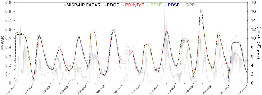
Remote Sens. 2020, 12, 3927                                                                             2 of 39

1. Introduction
     Vegetation regulates the carbon, energy, and water fluxes between the land and the atmosphere.
Plants affect and respond to environmental and especially climatic conditions: they typically exhibit
annual variations that match the seasonal evolution of temperature, water availability, solar irradiance,
and other critical variables. Hence, they are also sensitive to climate fluctuations and changes. Phenology,
the study of the seasonal evolution of plants, documents these variations and therefore provides evidence
of the impact of climate change on the environment.
     The Special Report on Emissions Scenarios (SRES) socio-economic CO2 emission scenario A2 of the
Intergovernmental Panel on Climate Change (IPCC) provides a suitable context to evaluate conditions
appropriate for the African continent. Under this scenario, Friedlingstein et al. [1] estimate that climate
warming during the 21st century may reduce the net ecosystem productivity of the African continent and
contribute up to 38% of the global climate-carbon cycle feedback. Properly characterizing vegetation’s
phenology is crucial to document this evolution and to accurately parameterize the global land-atmosphere
models [2]. In Southern Africa, air temperature near the ground has been increasing rapidly over the last
five decades, at about twice the rate of the globally average surface temperature [3–5]. These changes,
and associated fluctuations in the water cycle, are expected to have a significant impact on vegetation
cover in the savanna biome, which occupies about 20% of the global land surface and 40% of Africa,
according to Kutsch et al. [6].
     Phenology, may have notable economic implications, as plant growth and development depend
on the occurrence of essential weather events. Natural hazards, such as drought, flood, or fire,
can jeopardize agricultural yield in a given year, or sometimes the sustainability of that economic activity.
Phenology also informs on the land use and land cover type, providing useful information to manage
societies, their economic systems, as well as to monitor the evolution of unmanaged areas, such as nature
reserves. In the particular context of African ecosystems, savanna woody vegetation provides valuable
ecosystem services [7,8], and the effective estimation of those resources is required to satisfy commitments
to monitor and manage change within them [9].
     Repeated observations of the density and diversity of woody plant species in African savanna
regions suggest that variations in species composition and diversity are to a great extent also influenced
by land use and anthropogenic disturbances [10]. In South Africa, and in the Lowveld in particular,
rural households critically depend on fuelwood as a source of energy because of the prohibitive cost of
gas and fuels. This socio-economic constraint has resulted in the exploitation of natural resources well
beyond their capacity to regenerate, and therefore in the progressive deforestation of those environments.
That situation leads to wood scarcity, as well as potential, and, in many cases, actual, conflicts over access
to resources [11]; it is further exacerbated by a continuous exodus from rural areas to towns and cities,
as well as by immigration from neighboring countries. As a result, settlements have been expanding and
their environmental footprints have become more severe over time [12].
     This paper leverages two resources to bear on this problem: remote sensing and field measurements
to provide empirical evidence, and modeling to provide a rational framework for the interpretation of the
data, despite the uncertainties inherent to all measurements, the irregular distribution of observations in
time and missing data for various reasons. The aims of this methodological study were (i) to assess the
suitability of four parametric double S-shaped functions (the Gaussian, Hyperbolic Tangent, or Logistic and
Sine) to describe the phenology of savanna vegetation in the Lowveld, and (ii) to evaluate the capability of
these data and models to account for the Gross Primary Productivity (GPP) of the vegetation around the
Skukuza flux tower in South Africa’s Kruger National Park. This is of particular interest insofar as GPP is
one of the contributing factors to estimate biomass accumulation or yield (in an agricultural context).
Remote Sens. 2020, 12, 3927                                                                               3 of 39

2. Study Area
     The study site is centered on the Skukuza Eddy Covariance (EC) flux tower, which falls within the
Lowveld in the north eastern part of Mpumalanga Province of South Africa (Figure 1). The Lowveld
predominantly belongs to the large savanna biome, which covers one-third of the country. It is
characterized by hot humid summers and mild dry winters. Summer rains occur between October
and May across a west to east precipitation gradient, with a mean annual precipitation of 633 mm and
mean annual temperature of 21 C [13]. The Lowveld’s dominant geology includes granite and gneiss with
local gabbro intrusions [14]. The slopes and crests are characterized by a mixture of tall shrubland with
few trees to moderately dense low woodland, and valleys dominated by dense thicket and open savanna.
Vegetation distribution and density in the region are influenced by the rainfall gradient, geology, fire events,
mega-herbivore browsing, cattle grazing, and the anthropogenic harvesting of wood [14,15]. Coppicing is
prominent in areas which experience high levels of anthropogenic utilization [9]. Granite lowveld is
the main vegetation unit in the area, with dominant tree species, including Terminalia sericea, Combretum
zeyheri, Combretum apiculatum, Acacia nigrescens, dominant shrub species, including Dichrostachys cinerea
and Grewia bicolor, and dominant grass species, including Pogonarthria squarrosa, Tricholaena monachne,
Eragrostis rigidior, Panicum maximum, Aristida congesta, Digitaria eriantha, and Urochloa mossambicensis [13].

     Figure 1. Panel (a): Location of the study site in the Lowveld of South Africa with overlapping
     footprints of Multi-angle Imaging SpectroRadiometer (MISR) Block 110 for Path 168 (dotted rectangle)
     and 169 (full rectangle). Panel (b): Detailed map of the environment around Skukuza in the Kruger
     National Park. Source: South African National Biodiversity Institute (SANBI), acquired from https:
     //www.sanbi.org/link/bgis-biodiversity-gis/.

3. Data Collections

3.1. Satellite Measurements

3.1.1. Background
     Observations of land surfaces from spaceborne platforms started in earnest in the early 1970s with
the launch of the Earth Resources Technology Satellite (ERTS-1), subsequently renamed Landsat 1. In turn,
the availability of multispectral measurements stimulated the development of methods to explore the
significance and implications of those observations in practical applications. Rouse Jr. et al. [16] and [17]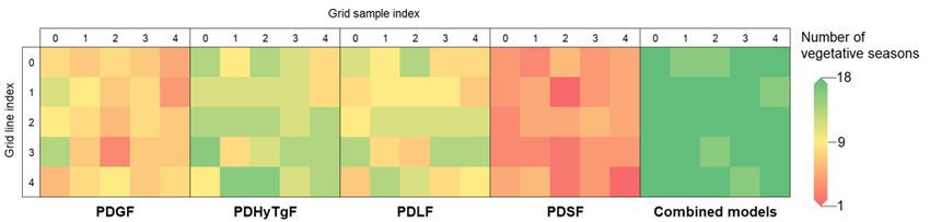
Remote Sens. 2020, 12, 3927                                                                               4 of 39

suggested that the ratio subsequently known as the Normalized Difference Vegetation Index (NDVI)
was adequate to monitor “the vernal advancement and retrogradation (Green wave effect) of natural
vegetation”, i.e., to monitor plant phenology as we understand it today. These events mark the start of a
sustained effort to monitor the biosphere on the basis of space observations [18].
     Over the past 50 years, significant progress has been achieved, and thousands of publications have
been published [19], to characterize the state and evolution of plant canopies using observations of the
reflectance of the planet in the solar spectral range. A full review of the literature dealing with the
documentation of plant phenology on the basis of remote sensing measurements is outside the scope of
this paper, but it is worth noting that progress has been achieved on multiple fronts:

1.    Major advances in understanding the processes of radiation transfer in complex environments resulted
      in the design and implementation of much improved algorithms. These aimed to effectively account
      for processes unrelated to vegetation (such as atmospheric clouds and aerosols, anisotropic effects,
      contributions to the measured signals due to variations in soil moisture, etc.) and to deliver reliable
      and accurate products to describe plant processes. The Fraction of Absorbed Photosynthetically
      Active Radiation (FAPAR) is a case in point, since it has been identified as one of the Essential Climate
      Variables (ECV) by the Global Climate Observing System (GCOS) [20]. These developments, in turn,
      led to a more quantitative representation of plant phenology (in [21–23]).
2.    The technology of measuring reflected radiation on spaceborne platforms has improved drastically,
      and is currently able to deliver up to hundreds of spectral bands at spatial resolutions of the order
      of tens of meters or less, sometimes on a daily basis, or to acquire data from multiple directions
      or in multiple polarizations. Data fusion with observations obtained with different instruments
      (e.g., LiDARs: see [24–26]) or in entirely different spectral regions (e.g., microwaves: see [27–29]) have
      also been explored, though much remains to be done in order to provide a holistic description of the
      environment, or of plant phenology in particular.
3.    Progress in the field of information technology delivered computing, networking and data archiving
      resources and capabilities orders of magnitude faster and more performant than even a few decades
      ago, and permitted the investigation of complex issues. Although the drive to acquire more and
      better observations continues unabated, the major bottleneck today concerns the actual analysis of
      those data and the extraction of useful information from the immense archives that have already been
      accumulated.

     As a result, Earth observing satellites have yielded a long-term record of changes in vegetation
photosynthetic activity, while ground-based eddy covariance measurements are providing automated,
continuous and spatially averaged measures of carbon exchanges between the surface and the atmosphere.
A global increase in ‘greening’ has been evidenced through remotely sensed indices, such as the
Leaf Area Index (LAI) and Normalized Difference Vegetation Index (NDVI), suggesting an increase
in the seasonally-integrated LAI of up to 25–50%, while less than 4% of the terrestrial areas exhibit a
decrease of LAI [30]. Key drivers of phenology include temperature and photoperiod in the mid- and
high-latitudes [2,31–33], while precipitation is regarded as the dominant driver in the tropics [34,35].
Satellite-based observations have been widely used to characterize the evolution of vegetation in the
Northern Hemisphere, but other regions have received far less attention: A systematic review of phenology
in Africa over the last decade reveals a recent increase in the number of phenological studies based on
remote sensing but suggests that further investigations are needed across this continent, especially to focus
on the relationship between climate and vegetation phenological changes [36].
     Remote sensing research in the Lowveld has tended to focus on the use of mono-directional spectral
measurements (from airborne and/or spaceborne sensors) which typically inform on the chemical
composition of the targets (in [37–40]). More recently, sporadic airborne campaigns collecting Light
Remote Sens. 2020, 12, 3927 5 of 39
Detection And Ranging (LiDAR) measurements have been used to document the structural properties
of the vegetation canopies, e.g., to map the differences in canopy and sub-canopy cover height and
distribution [26,41,42]. One of the main advantages of using LiDAR observations is the ability to capture
sub-canopy structural changes specifically to examine bush encroachment, otherwise unattainable in
mono-directional spectral measurements which only account for the aerial extent of the vegetation
canopy [43]. Hybrid techniques combining structural observations from LiDAR and spectral measurements
from hyperspectral and multispectral data sets demonstrate the ability to classify individual tree
species [25,44]. To a lesser extent, Advanced Synthetic Aperture Radar (ASAR) measurements, which can
observe the surface irrespective of the cloud cover, have been used to create regional scale baseline
maps of savanna woody cover in the Lowveld [9]. Cutting-edge approaches utilizing LiDAR, ASAR,
and hybrid-techniques are very interesting but infrequent and limited in geographical scope, constrained in
part by the limited spatial coverage and the cost of obtaining the data sets.
3.1.2. Multi-Angular Observations
Anisotropy is typically considered a source of noise when analyzing remote sensing data from
mono-angular spectral instruments but constitutes a definite advantage when analyzing measurement
from multi-angular instruments [45]. Over the last three decades, the potential benefits of multi-angular
observations have been recognized through the operation of innovative Earth Observation (EO)
instruments, such as the Along-Track Scanning Radiometer (ATSR-1 and ATSR-2), the Polarization and
Directionality of the Earth’s Reflectance (POLDER), and the Multi-angle Imaging SpectroRadiometer
(MISR) instrument on-board National Aeronautics and Space Administration (NASA)’s Terra platform,
which has been continuously operating since 24 February 2000. These instruments generate an improved
characterization of the atmospheric and terrestrial environments because multi-angular measurements
permit an accurate, quantitative decoupling of the distinct spectral and directional signatures of those
geophysical media.
In this context, the recent availability of land surface products at the relatively high spatial resolution
of 275 m generated by the MISR-HR (for High Resolution; version 2.01-0) processing system [46],
about weekly over the period 2000–2018, offers new opportunities to explore the relation between
surface properties and the fluxes of matter and energy in the environment. Appendix A summarizes the
specifications of the MISR instrument and outlines the products generated by the MISR-HR processing
system. Specifically, the Joint Research Centre-Two-stream Inversion Package (JRC-TIP) algorithm [47,48]
derives the Fraction of Absorbed Photosynthetically Active Radiation (FAPAR) product from an analysis
of albedo values obtained by integrating the Rahman-Pinty-Verstraete (RPV) model [49,50]. FAPAR is a
measure of the absorption of incoming solar radiation in the canopy, within the photosynthetically relevant
spectral region (400 to 700 nm) (in [51,52]). The JRC-TIP inversion process returns the final value of the
cost function, as well as estimates of the variance, associated with each product: the former is a measure of
the distance between the model and the data, while the latter measures the uncertainty associated with the
retrieved product.
3.1.3. MISR-HR FAPAR Product for Skukuza
This MISR-HR FAPAR product has been extensively evaluated [53–56] and serves as a benchmark
in various contexts, as noted earlier. It also offers three advantages over the traditional NDVI used
in many phenological studies: (1) FAPAR is much better grounded in radiation transfer theory and
has been identified as an “Essential Climate Variable” by the GCOS, which is not the case for NDVI,
(2) this particular product is derived using the JRC-TIP algorithm, a state of the art inversion procedure
that has been extensively validated (see, e.g., https://fapar.jrc.ec.europa.eu/Home.php, last visited onRemote Sens. 2020, 12, 3927 6 of 39
21 November 2020), and routinely used by the Committee on Earth Observation Satellites (CEOS) Working
Group on Calibration and Validation (WGCV) and the European Commission Quality Assurance for
Essential Climate Variables (QA4ECV) project, for instance, and (3) this product is made available at a
higher spatial resolution (275 m) than any of the traditional global vegetation index products (500 m at
best, and often 1 km or more) available over the last 20 years.
The Skukuza flux tower site falls within Block 110 of MISR Paths 168 and 169 (Figure 1, panel (a)).
The repeat period of this instrument for a single Path is exactly 16 days, but the study area is located
within the overlap of those Paths, giving a staggered revisit period of seven and nine days between those
two Paths. A total of 859 combined Orbits for both Paths (i.e., 429 and 430, respectively) were acquired
between 15 March 2000 and 30 December 2018; 17 of them were irretrievable from NASA’s Atmospheric
Science Data Center (see https://asdc.larc.nasa.gov/project/MISR/, last accessed on 14 October 2020.),
due to technical issues with the platform. As a result, the longest period between successive acquisitions is
32 days. However, cloudiness further reduces the availability of usable surface observations, so the time
gaps between successive observations is typically 7 or 9 days during the dry season, but may reach up to
100 days or more during the wet season.
The MISR-HR FAPAR product is made available on the Space Oblique Mercator (SOM) map projection,
like all standard MISR data products. This projection minimizes shape distortion and scale errors
throughout the length of the Orbit near the satellite ground track. However, each Path possesses its
own unique SOM map projection parameters, so assembling data sets involving two or more Paths imply
re-projecting the data onto a common grid, in this case, the geographic spatial reference system, i.e.,
European Petroleum Survey Group (EPSG) code: 4326, as explained below in Section 4.2.2.
3.2. Flux Tower Observations
Flux towers use micrometeorological measurements and the Eddy Covariance (EC) method (first
published by [57]) to directly observe air motion and gas concentrations at two or more heights, and to
estimate the exchanges of gas, energy, and momentum between the terrestrial biosphere and the overlying
atmosphere on an ecological scale from the covariance between fluctuations in those variables [58–60].
GPP (expressed in units of gC m−2 d−1 ) is derived from an analysis of those data. Figure 2 shows the
relation between the GPP and precipitations, in this case, estimated as part of the European Centre for
Medium-Range Weather Forecasts (ECMWF) Re-Analysis (ERA)-Interim reanalysis project.
It is important to note, from the outset, that unmanaged, protected areas in a National Park are not
monitored or used like an agricultural field: there is no planting or harvesting date, and nobody observes
the emergence of leaves or flowers. This would be difficult in any case, given the diversity of species
involved. Hence, the characterization of the phenology of the canopy must be derived from remote sensing
measurements and access to local observations from an EC flux tower provides a unique opportunity to
establish possible relations between remote and in situ measurements, even though these address quite
different biogeophysical variables.
The Skukuza EC flux tower is located at 25◦ 10 10.5400 S, 31◦ 290 48.600 E within the Kruger National Park,
near the Skukuza camp, at an altitude of 365 m above sea level. It has been in continuous operation since
2000, and stands on the ecotone between broad-leafed Combretum savanna on sandy soil and fine-leafed
Acacia savanna on clayey soil [61]. Woody vegetation height ranges between eight and ten m, and the flux
sensors on the tower are 17 m above ground, implying a sensor footprint of about 500 m [62]. The Skukuza
flux tower currently makes use of the LiCor 7500 open-path infrared gas analyzer to measure carbon
dioxide (CO2 , µmol mol−1 ) and water vapor (H2 O, mmol mol−1 ) concentrations, as well as ultrasonic
anemometers (Gill Wind Master Pro and Campbell Scientific CSAT3), to measure horizontal and vertical
fluctuations in wind speed (m s−1 ) and air temperature (K).Remote Sens. 2020, 12, 3927 7 of 39
NASA erected this flux tower as part of the Southern African Regional Science Initiative
(SAFARI–2000), an international field campaign investigating emissions, transport, transformation and
deposition of trace gases and aerosols over southern Africa between 1999 and 2001 [61,63–65]. The tower
was subsequently donated to the Council for Scientific and Industrial Research (CSIR).
Figure 2. Time series of daily values for the Gross Primary Productivity (GPP) of the unmanaged vegetation
around the Skukuza Eddy Covariance (EC) flux tower (in red) and the daily precipitation estimated by the
ERA-Interim reanalysis data accompanying the FLUXNET2015 archive.
The Skukuza EC flux tower measurements confirm the close inter-connection between the water and
carbon fluxes: ecosystem respiration is highest at the onset of the wet season, continuously decreasing
during the transition towards the dry season [6]. Variations in precipitation between years, which influence
variations in the amount of green leaf area, seasonal patterns, and soil water availability are the main
drivers of Net Ecosystem Exchange [62]. This approach has been used to estimate GPP [66], as well as to
partition the energy fluxes, at the surface [67].
For the purpose of this study, the Skukuza flux tower data set processed by the FLUXNET organization
(Site Id: ZA-Kru) was downloaded from the FLUXNET2015 data archive (Available from the portal
https://doi.org/10.18140/FLX/1440188, last accessed on 14 October 2020.). This organization coordinates
regional and national networks to harmonize the compilation, archival and distribution of data to the
scientific community. It comprises over 900 flux tower sites globally (See https://fluxnet.fluxdata.org/,
last accessed on 14 October 2020.). Data were originally released in December 2015 and subsequently
updated in July 2016 and November 2016, following the procedures and quality controls described
in [68,69]. The ERA-Interim global reanalysis data set of the European Centre for Medium-Range Weather
Forecasts (ECMWF) is used to fill extended gaps of micrometeorological variable records. These data are
distributed under the CC-BY-4.0-based data policy (See https://creativecommons.org/licenses/by/4.0/,
last accessed on 14 October 2020.).
The reliability of phenological information derived from satellite remote sensing observations is
evaluated by confronting them to flux tower results [70,71]. The availability of both remote sensing and
field measurements at the Skukuza site thus offers a unique opportunity to characterize the phenology of
that biome.
4. Data Processing
4.1. Measurement Uncertainties and Missing Data
Each plant species typically follows its own phenological development, itself dependent on the locally
prevailing conditions. For their part, spaceborne EO instruments acquire measurements (usually overRemote Sens. 2020, 12, 3927 8 of 39
areas large with respect to the dimensions of plants, hence containing many plant species), over periods
of time which may or may not coincide with the specific observational needs at any given location.
Individual observations are associated with measurement uncertainties, which result from systematic,
as well as random, errors, due to incorrect or biased calibration, and intrinsic limitations on the precision
of the instrument, respectively. In addition, optical instruments measure the combined contributions of the
planetary surface and the overlying atmosphere: clouds and aerosols can perturb or prevent observations
of the surface. Measurements actually useful to characterize the phenology of plant canopies are therefore
scattered in space and time, especially during rainy seasons [72].
Models, such as the ones described below, are required to provide a reliable representation of the
phenology of plant canopies despite these challenges. Once they have been adjusted to optimally fit
the available empirical evidence, they can be used to provide a simplified stable characterization of
the evolution of plant canopies. The combined empirical evidence on phenology derived from remote
sensing and ground-based observations has been shown to improve the accuracy of models simulating
surface-atmosphere interactions (in [73–75]).
4.2. Pre-Processing
4.2.1. Screening Outliers
The reliability of an analysis based on measurements clearly depends on the accuracy of the inputs,
so outliers and doubtful items should be culled out of the data. As explained above and in Appendix
A.2, FAPAR values are themselves obtained through a model inversion procedure, and their accuracy
and reliability can be quantitatively assessed by inspecting two pieces of information: the variance
associated with the reported values, and the value of the cost function at the end of the inversion process.
Whenever the latter exceeds a given threshold (in this case, set to the 90th percentile of its distribution),
the mismatch between the model and the empirical evidence is deemed excessive and the corresponding
data items are discarded, following the approach described in Liu et al. [76]. This is preferable to traditional
statistical methods (such as box-and-whisker statistics) because it eliminates not only obvious outliers
but also data values that may look reasonable but are probably questionable: a high cost function value
betrays a mismatch between the JRC-TIP model and the input data and often results in one or more of
the model parameters taking on unusual or obviously unbelievable values. This process, thus, tends to
discard more data points than would be eliminated on the basis of extreme values only but yields a time
series of high quality.
The threshold of acceptability can be fine-tuned by inspecting the histogram of cost function values,
which typically exhibits a long tail of occasional large values, so the selection of a particular value within
that tail is not very crucial, as it screens out a small number of points. Figure 3 shows that keeping data
points associated with slightly higher cost function values (for instance 0.12 instead of 0.10) would add a
few more data points to the time series, though most of them cluster in late 2016 and early 2017, at a time
when they would not provide much additional constraint on the model inversion. Selecting much smaller
values does have a significant impact on the number of remaining data points, as documented in Table 1.
In practice, the choice should be driven by the requirements of the user of the information: is it better to
have very reliable data on a smaller number of cases, or more approximate and potentially less reliable
information more frequently? The interesting feature of this approach is that there is no need to impose a
single solution for all possible problems: the process can be customized to meet the specific requirements
of the user.Remote Sens. 2020, 12, 3927 9 of 39
Figure 3. Time series plots showing how a threshold value of the cost function distribution (in this instance
0.1) flags obvious and less apparent cases of problematic values in Fraction of Absorbed Photosynthetically
Active Radiation (FAPAR) in the time series at the reference pixel of the Skukuza flux tower and for MISR
Paths 168 and 169.
Figure 3 shows the outcome of this process in a particular case: The top panel exhibits the time series
of FAPAR values for the Skukuza flux tower for Paths 168 and 169, while the bottom panel shows the
associated JRC-TIP cost function values. In this case, the threshold of acceptable cost function values is set
to 0.1. All cost values larger than this threshold and the corresponding FAPAR values in the top panel,
are marked in red. This process eliminates the occasional slightly negative FAPAR values, but also other
values that might otherwise appear to be reasonable at face value. Of course, a lower threshold would
prune even more data points and jeopardize the feasibility of characterizing the vegetative season, while a
larger threshold would retain more data but possibly lead to an incorrect interpretation because of the
presence of dubious values.
Table 1 shows how selecting progressively stricter threshold values for the cost function increases
the number of data points considered outliers or potentially suspicious and decreases the number of data
points remaining available for further analysis.
Table 1. Relation between the largest allowable cost function value (Threshold), the number of data points
identified as outliers, and the number of data points remaining available for further analysis in the time
series of Figure 3.
Threshold 0.1 0.08 0.06 0.04
Outliers 34 59 110 211
Remaining 303 278 227 126
Figure 4 exhibits the histogram of the FAPAR values in the five-by-five pixel area around Skukuza
for Paths 168 and 169 (a) before screening outliers (indicated in red), and (b) after discarding values
associated with an excessive cost function value for those pixels (depicted in blue). The average costRemote Sens. 2020, 12, 3927 10 of 39
function threshold for all pixel locations in the FAPAR record was 0.099, which resulted in about 10.7% of
the values in the image time series being discarded.
Figure 4. Histogram of FAPAR values for the area surrounding Skukuza and for Paths 168 and 169 (a) before
screening outliers and (b) after discarding outliers using a threshold value of the cost function (0.099).
Figure 5 summarizes the number of valid FAPAR values available per month, for each year in the
record, averaged over the target area around the Skukuza flux tower. It can be seen that remote sensing
observations are most often lacking during the wet season (December to March), due to the prevailing
cloudiness. The longest continuous period without any observations in this particular case can last up to
four months, as happened between October 2009 and January 2010, and between December 2011 and March
2012, inclusive. This situation would be even worse close to the Equator, both because of the prevailing
cloudiness and because of the minimal overlap between consecutive MISR Paths. Contrariwise, at higher
latitudes, in both hemispheres, a larger overlap between Paths provides more frequent opportunities to
observe the surface.
Figure 5. Distribution of the availability of the number of valid FAPAR values as a function of month (along
the vertical axis) and year (along the horizontal axis), averaged over the target area around the Skukuza
flux tower.Remote Sens. 2020, 12, 3927 11 of 39
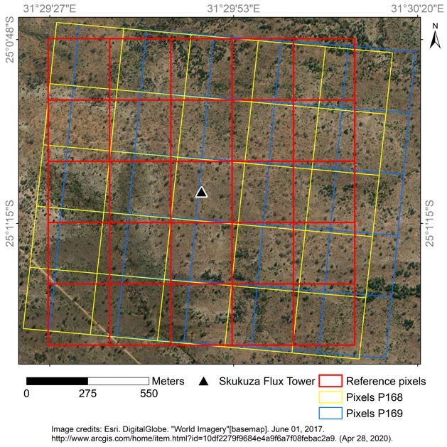
4.2.2. Assembling the FAPAR Data Cube
The next step consists in merging data from the two relevant MISR Paths. Raster images of five
samples by five lines, centered on the geographic location of the flux tower, were extracted from the
FAPAR product for each of the 842 available Orbits and reprojected onto a common geographical grid,
since both the MISR data and the MISR-HR products are provided in the SOM projection specific to each
Path. Figure 6 explains this process graphically: Three grids are superimposed on a background map of
the area around Skukuza, symbolized by the black triangle at the center of the display: the yellow and
blue grids show idealized representations of the locations of the areas observed by MISR in Path 168 and
169 acquisitions, respectively. The red grid is the common geographical projection used as the target, and all
grid squares are 275 m on the side, the ground sampling distance of MISR-HR products. This process
roughly doubles the number of observations at each location, and helps constrain the phenology.
4.2.3. Identifying Individual Vegetative Seasons
The successive vegetative seasons must be identified before attempting to fit a double S-shaped
model through the data, accounting for the fact that their growth and senescence phases can start and
last differently in different years, mostly as a result of climatic fluctuations. This process is implemented
as follows. A power spectrum for the entire time series is computed first, using the Lomb-Scargle
algorithm [77,78] since the remote sensing data are provided on irregular dates. The resulting periodogram
indicates whether the record exhibits primarily an annual variation (as is the case in Skukuza), or a biannual
cycle, as would occur in agricultural regions where two crops can be grown per year. Figure 7 shows the
Lomb periodogram for the FAPAR time series at the pixel location of the Skukuza Flux tower. This area
exhibits a strong annual cycle (peak power: 71.72, frequency: 0.0027 day−1 , and period: 364.75 days) and a
minor semi-annual fluctuation (peak power: 16.63, frequency: 0.00548 day−1 , and period: 182.37 days).
Figure 6. The pixel reference grids used to co-register the MISR-HR FAPAR variable for Paths 168 and
169 of Block 110 to geographic coordinates for the Skukuza flux tower.Remote Sens. 2020, 12, 3927 12 of 39
Figure 7. Lomb periodogram of the FAPAR time series at the reference pixel of the Skukuza flux tower.
Since satellite records may start and end at arbitrary times relative to climatic or ecological cycles,
the second step consists in identifying the start of the first complete vegetative season that can be
documented on the basis of the data record. This is achieved as follows:
• compute the median of the entire FAPAR record,
• search, from the start of the record, the date of the first observation whose value is lower than this
threshold,
• define a time interval equal to 1/3 of the expected length of the vegetative period (as determined
from the Lomb-Scargle algorithm), starting on this date, and
• set the start date of the first vegetative season to the date of acquisition of the minimum FAPAR value
within this limited time period.
From that point onwards, the end date of each vegetative season is automatically considered the start
of the next one. The end of each season date is determined as follows:
• add the expected average length of the vegetative season to the starting date just identified to estimate
a nominal end date,
• define a new limited time window located around that nominal end date, extending 1/6 of the
expected length of the vegetative season on either side of that nominal date, and
• set the end date of the vegetative season to the date of acquisition of the minimum FAPAR value
within this limited time period.
This process is repeated until the nominal date of the end of the nth vegetative season exceeds the
length of the remote sensing record. As a result, some data may be discarded at the start and end of the
entire record, since they only document parts of vegetative seasons.
Figure 8 plots a subset of the FAPAR time series at the pixel location of the Skukuza flux tower,
showing the first few years of the MISR-HR FAPAR time series: the vegetative season ending in August
2000 is ignored because it is incomplete, and the next three are properly identified. The successive search
periods are indicated by the blue dotted lines, and the red lines mark the start and end dates of the
vegetative seasons.Remote Sens. 2020, 12, 3927 13 of 39
Figure 8. A subset of the FAPAR time series at the reference pixel for the Skukuza flux tower showing
the start of the first vegetative season between 2000 and 2001 and the vegetative seasons for 2001–2002,
2002–2003, and 2003–2004. The dotted blue lines delimit the search periods for the start and end of the
vegetative seasons, and the solid red lines indicate those boundaries. The dashed green line represents the
median value for the record, in this case, 0.25.
4.3. Modeling Phenology
Once each individual vegetative season has been identified, the evolution of the plant canopy
properties during that period can be modeled. This is beneficial (i) to estimate the timing of events, such as
the start, end, and length of the season (SOS, EOS, and LOS, respectively), (ii) to document the probable
value of biogeophysical variables, such as FAPAR, when direct observations are missing, and (iii) to
characterize the long-term evolution of the environment, in this case, for the environment around the
Skukuza flux tower, in the Lowveld savanna of north-eastern South Africa, during the period 2000–2018,
despite the presence of noise in the data.
Global and local methods have been used in the literature for similar purposes. Local approaches
take existing data at face value and generate estimates of missing observations on the basis of the values of
neighboring measurements [79]. They include rank based filters, e.g., minimum, median, and maximum
filters [80], linear/polynomial filters, such as moving average and adaptive Savitzky-Golay filters [81–83],
locally weighted scatterplot smoothing (in [79,84]), and Whittaker smoother (in [85]) to name a few.
Advantages include the applicability to any time series, irrespective of their semantic or thematic context,
and an ability to match arbitrary fluctuations, but at the risk of simulating fluctuations that may be
suggested by noisy or erroneous data.
Global models, by contrast, impose a functional shape that is intended to represent the likely evolution
of the variable of interest, in this case, the phenology of vegetation, which is expected to exhibit a growth
phase, followed by a senescence phase. They include function-fitting approaches, e.g., polynomial,
double logistic, asymmetric Gaussian [86–89], and signal smoothing or decomposition techniques, e.g.,
wavelet transform, Fourier analysis, Lomb-Scargle [90–95]; see [79]. Signal decomposition techniques
provide forecasts over a season by decomposing the time series into noise, seasonal variability and
trend [96]. The Lomb-Scargle algorithm, initially developed by Lomb [97] and subsequently elaborated
by [98], implements an approach similar to Fourier analysis [99], adapted to estimate the power spectral
density of unevenly sampled data [77,78].
Local and global phenology models both have advantages and drawbacks: The selection of a global
versus a local model must depend on the intended usage of the resulting information. Global models are
deemed particularly suited to represent the temporal evolution of vegetation when the empirical evidence
exhibits unusual or unexpected fluctuations (as is the case here): they are used as low-pass filters to screen
out the influence of extraneous or uncontrolled processes, such as biomass burning, random browsing,
the possible contamination due to thin clouds or aerosols, or simply noise in the data. A local modelingRemote Sens. 2020, 12, 3927 14 of 39
approach would definitely be more appropriate if the objective were to specifically monitor biomass
burning events, for instance.
This study explores the suitability of four different global models, each constructed as a pair of
S-shaped functions (one to simulate the growth phase and the other to represent the senescence phase):
Gaussian, hyperbolic tangent, logistic (these two functions are mathematically equivalent, but they exhibit
differences in terms of numerical efficiency, as will be shown below), and sine. Of those four models,
the logistic function has been used most frequently in phenology (and other ecological) studies (in [21,
34,88]). A smaller number of investigations explored the suitability of the hyperbolic tangent [100–102],
probably because of its similarity with the logistic function. Rather fewer researchers seem to have
considered the Gaussian [103,104] or the sine functions. This paper aimed in part to explore which of those
formulations might be more appropriate or more advantageous for this purpose.
These four mathematical models are described in detail in Appendix B. The shape of each elementary
S-shaped function is determined by four independently adjustable parameters, typically to specify the
(Julian) date and value of the start and of the end of the simulated fluctuation. Imposing a continuity
condition between the two functions of each pair reduces the number of parameters to be adjusted to
seven. The process of fitting a double S-shaped model to the data reduces to an inversion procedure,
where the goal is to optimize a goodness of fit criterion: it is typically implemented as an iterative
algorithm to minimize a figure of merit function, such as the root mean square difference between the
model and the observed values (χ2 ). When this condition is realized, the values of the model parameters
are deemed to optimally describe the seasonal evolution of the simulated geophysical variable, and the
model, together with these newly established parameters, can be used to generate a complete time series,
at whatever frequency is required.
Data points can be assigned weights during this inversion process, to allow those with smaller
uncertainties to have more influence on the outcome than points with larger uncertainties. The inverse
of the estimated standard deviation provided by the JRC-TIP algorithm for each FAPAR value was used
as the weight in this investigation. The iterative inversion process is terminated when the value of χ2
changes by less than 10−3 between successive iterations, i.e., when there is little benefit to be gained by
searching for another minimum in the current neighborhood.
This approach requires at least four FAPAR values within each of the growing and decay phases,
and more than seven values over the entire vegetative season to ensure that the number of measurements
exceeds the number of model parameters to be determined [105]. The average number of valid FAPAR
observations across all pixel locations in the FAPAR record is 288, which, over a period of 18 years,
yields around 16 observations per season. However, those are very unevenly distributed, with many
more data points during the dry season (under clear skies) than during the rainy season, as was shown in
Section 4.2.1. In fact, the process of inverting the models against those data can fail or lead to unrealistic
results whenever there are fewer than four observations during the growing phase, which is always the
most cloudy.
In addition to systematically fitting each of these double S-shaped models to each vegetative season,
a combined approach was also explored, whereby the best model for each individual season is selected,
to increase the number of successful model inversions and decrease the average χ2 statistic.
Once a parametric double S-shaped model has been successfully fitted to the remote sensing
measurements, classical techniques based on an inspection of the first and second derivative of this
model can be used to determine the start, end, and length of the growing season (in [22,106], among many
others).Remote Sens. 2020, 12, 3927 15 of 39
5. Results and Discussion
This section documents the results obtained from the application of the methods described in Section 4
to the data sets identified in Section 3. Section 5.1 discusses to what extent the parametric double S-shaped
models are capable of representing the phenology of vegetation as reported by MISR-HR FAPAR time
series. Section 5.2 explores the effectiveness of this joint approach to document the ecological evolution of
the target area by comparing those results with the Gross Primary Productivity (GPP) estimates derived
from in situ measurements at the Skukuza flux tower. Section 5.3 reports on the numerical efficiency of
these algorithms, while Section 5.4 summarizes the results.
5.1. Simulation Capability
All four parametric double S-shaped models are capable of simulating a seasonal signal when the
number of data points is large enough to individually document the growth and senescence phases.
Each of those models relies on seven adjustable parameters to match the empirical evidence, so eight
measurements are required at a minimum before attempting to invert the model against the data for a
particular season. It is generally easy to document the evolution of the phenology during the dry season,
i.e., when the vegetation senesces or becomes dormant. The difficulty arises when persistent cloudiness
generates long gaps in the remote sensing measurements during the rainy season, precisely when the
vegetation grows. Figure 9 exhibits the number of FAPAR values available per year over the target of
interest for the entire record available.
Figure 9. Boxplots summarizing, for the entire MISR-HR FAPAR record, the number of observations
available per year to fit the model during (a) entire vegetative seasons, (b) the growth phase, and (c) the
senescence phase. The top and bottom limits of the boxes show the quartiles, the horizontal line in the
middle of those boxes and the crosses indicate the median and the average values, respectively, while the
‘T’ shaped extensions document the range of values (minimum and maximum).
As expected, there are fewer observations during the rainy season (growth phase). Whenever too
few FAPAR values are present during the growth (more rarely senescence) phases, the inversion process
fails. It is interesting to note that the various models exhibit different sensitivities to the presence of thoseRemote Sens. 2020, 12, 3927 16 of 39
data gaps. Figure 10 summarizes the number of successful inversions for each of the four models in the
target area.
Figure 10. Number of successfully simulated vegetative seasons. The four left-most panels report the
results for the Parametric Double Gaussian Function (PDGF), Parametric Double Hyperbolic Tangent
Function (PDHyTgF), Parametric Double Logistic Function (PDLF), and Parametric Double Sine Function
(PDSF) models, respectively. The fifth panel shows the success rate when the most successful model is
selected for each season at the sample and line locations in the target area.
It can be seen that the hyperbolic tangent model offers the most frequent opportunities to successfully
simulate a vegetative season, as well as that the sine model is the most sensitive to the presence of gaps in
the data, i.e., to the temporal distribution of empirical data throughout the season.
5.2. Ecological Effectiveness
Comparisons between models adjusted to fit remote sensing data and in situ field measurements
must take place over approximately similar areas. Since the Gross Primary Productivity (GPP) estimates
derived from flux tower Eddy Covariance (EC) measurements are deemed to be representative of an area
of approximately 500 m around the tower (an area of 53.5 ha), the FAPAR product is averaged over the
subset of 3 by 3 pixels centered on the Skukuza flux tower (an area of 68.1 ha). The corresponding average
standard deviation for each date in the remote sensing time series is computed as the square root of the
average variance of the nine pixel values. The four models described earlier are then adjusted to this
spatially averaged time series, and the results are described in the following subsections.
5.2.1. Comparing Daily Values
Figure 11 exhibits multiple time series at once, over the period September 2000 to August 2013,
when the GPP data are available: the little circles represent the 215 average FAPAR values available for that
period, estimated as explained above. The four sets of smooth colored dashed curves represent the model
fits, and the highly variable grey trace shows the daily values of GPP, derived from the Skukuza flux tower
EC measurements. The traces of the four models largely overlap each other when the temporal distribution
of the FAPAR data is adequate and when all models exhibit a very similar performance in simulating the
phenology (for seasons peaking in early 2002, 2003, 2004, 2006, 2009, and 2013). By contrast, during the
seasons peaking in early 2001, 2005, 2007, 2008, 2010, 2011, and 2012, the Parametric Double Sine Function
(PDSF) model did not converge to a useful solution, so its trace is absent from the Figure. In these latter
cases, it can be seen that the traces of Parametric Double Hyperbolic Tangent Function (PDHyTgF) and
Parametric Double Logistic Function (PDLF) coincide, as well as that the Parametric Double Gaussian
Function (PDGF) model delivered a different simulation, clearly distinguished from the other two.Remote Sens. 2020, 12, 3927 17 of 39
Figure 11. Superposition of multiple time series, from September 2000 to August 2013: the FAPAR
data (small circles, non-dimensional), averaged over a 3 by 3 pixel area around the Skukuza flux tower,
the four model fits (smooth colored curves, non-dimensional), each adjusted to fit the remote sensing data,
and the daily GPP values derived from the in situ Eddy Covariance (EC) measurements (jagged grey trace,
in gC m−2 d−1 ).
Table 2 quantifies the correlation between daily FAPAR estimates generated by the four models
(PDGF, PDHyTgF, PDLF, and PDSF) and the corresponding daily GPP record retrieved from an analysis
of the EC flux tower, for each of the 13 vegetative seasons available. The first column reports the dates
of the start and end of those seasons and the second refers to the season number. The third and fourth
columns indicate the number and the proportion (in%) of days in the corresponding seasons for which
GPP measurements were available, respectively. The next four columns report the Pearson correlation
coefficient between model-generated daily estimates of FAPAR and the daily GPP values derived from in
situ measurements for the same days. The last column shows the same statistics for the combined model,
i.e., when the best (smallest χ2 ) model is chosen for each year. Label A in the four model columns flags
cases where fewer than half of the daily GPP values were available for the concerned season (as shown in
the fourth column, and also in Figure 11). Label B in those columns flags cases where the model values
are unavailable, typically because the temporal distribution of the FAPAR data did not permit the model
inversion. Vegetative season numbers set in bold face within the second column point to cases where the
number of daily GPP was sufficient (more than 50% of the days) and where all four parametric double
S-shaped functions could be successfully inverted against the FAPAR data.
Correlation coefficients between the daily GPP and daily estimates derived from the PDGF, PDHyTgF,
PDLF and combined model approaches are always equal to or larger than 0.69 in seasons 2 to 5 and 9 to
12. This coefficient is much lower in the case of season 1 because (1) a long gap in the remote sensing
data, due to persistent cloudiness, hampers the model inversion procedure and (2) the GPP data suggest
a noticeable but unexpected double vegetative season during that period, unconfirmed by the remote
sensing record. The number of daily GPP measurements available in seasons 6, 7, and 8 was too low to
compute that statistic. Season 13 was also exceptional in two other ways: (1) the FAPAR data includes an
anomalously low value near the peak of the growing phase (possibly due to incomplete or insufficient
cloud screening), while the GPP data suggests a sustained activity throughout the period. The PDSF
model, for its part and in its current implementation, appears to be more sensitive to the distribution of
data points during the season than other models. However, when the model inversion does work, it tends
to yield very good results.
Figure 12 shows the non-linear relation between daily simulated FAPAR and daily GPP measurements
across all seasons, as represented by each of the indicated models: remote sensing measurements (in this
case, of FAPAR) appear quite sensitive to small variations of GPP when the latter is itself low (i.e., at theRemote Sens. 2020, 12, 3927 18 of 39
start an end of the vegetative seasons), as well as tends to saturate during the peak of the growing phase.
This finding may need to be confirmed in other locations but suggests that FAPAR is a sensitive indicator
of GPP in the range of 0 to 5 gC m−2 d−1 but then saturates and is not usable to estimate larger carbon
exchanges.
Table 2. Correlation coefficients (r) between the daily GPP and daily FAPAR estimates from the PDGF,
PDHyTgF, PDLF, PDSF, and combined models for each vegetative season and for the area around the
Skukuza flux tower. Entry A indicates that fewer than half of the expected GPP values were available,
while entry B means that the model could not simulate the available FAPAR data.
Vegetative Season GPP PDGF PDHyTgF PDLF PDSF Combined
SOS/EOS
Season Length % r r r r r
2000–08–31
2001–09–10 1 375 99.2 0.56 0.52 0.52 B 0.56
2002–10–24 2 409 86.8 0.72 0.78 0.78 0.74 0.72
2003–08–31 3 311 100 0.71 0.70 0.70 0.70 0.71
2004–09–18 4 384 100 0.81 0.82 0.82 0.82 0.81
2005–08–20 5 336 94.6 0.92 0.93 0.93 B 0.93
2006–07–15 6 329 24.9 A A A A A
2007–08–10 7 391 41.4 A A AB AB A
2008–09–06 8 393 45.3 A A A AB A
2009–09–16 9 375 82.1 0.79 0.80 0.80 0.80 0.79
2010–08–27 10 345 100 0.69 0.72 0.72 B 0.69
2011–09–06 11 375 100 0.80 0.82 0.82 B 0.80
2012–09–01 12 361 100 0.82 0.80 0.80 B 0.82
2013–08–26 13 359 100 0.56 0.56 0.56 0.55 0.56
However, Figure 11 also shows why that relation is complex: daily model values for seasons 4 and
5 are very similar, while daily GPP values in season 5 are almost double the values in season 4.
The impact of lacking remote sensing evidence on the shape of the model can also be highlighted
by comparing seasons 10 and 11: In those cases, the GPP daily values are comparable but the absence of
observational constraint near the peak of the season probably resulted in substantial overestimations by
the model in season 11.
Figure 12. Scatterplot of daily FAPAR estimates (when the PDHyTgF model successfully simulates
vegetative seasons) versus daily GPP (gC m−2 d−1 ) values when at least half of the expected values are
available (i.e., season 2, 3, 4, 9, 10, and 12).Remote Sens. 2020, 12, 3927 19 of 39
5.2.2. Comparing Seasonally Integrated Values
A high correlation between daily FAPAR values (retrieved from remote sensing or simulated) and daily
GPP estimates (derived from flux tower measurements) is not expected because the former correspond to
instantaneous assessments of the reflectance of the canopy, while the latter accounts for the evolution of that
canopy throughout the day. In situ observations are also sensitive to a wide range of local perturbing factors
that do not affect the observations gathered from space, such as wind speed and direction, for instance.
On the other hand, it is customary to integrate these time series over the lengths of vegetative seasons.
This approach tends to reduce the inherent variability of those signals (mainly the GPP in this case) and to
focus on the seasonal environmental properties rather than the daily fluctuations. Table 3 shows the result
of this process: The first two columns are the same as for Table 2; the third one shows the integrated GPP
value for the specified seasons, and the next four columns provide the integral of the four models over
these same seasons, again using the results obtained for the spatially averaged 3 by 3 pixel area around the
Skukuza flux tower.
Table 3. Correlations coefficients (r) between the integrated GPP and Cumulated FAPAR (CFAPAR)
obtained by integrating the PDGF, PDHyTgF, PDLF, PDSG, and combined models during the indicated
vegetative seasons. Computations were skipped whenever fewer than half of the expected GPP observations
were available during the season, or when the correlation between the daily GPP and model values dropped
below 0.70 in Table 2 (see text for details).
Vegetative Integrated CFAPAR
SOS/EOS
Season GPP PDGF PDHyTgF PDLF PDSF Combined
2001–09–10
2002-10-24 2 815.25 117.72 122.26 122.26 118.50 117.72
2003–08–31 3 656.65 84.19 84.14 84.14 84.40 84.19
2004–09–18 4 682.33 119.50 119.91 119.91 119.24 119.50
2005–08–20 5 1043.88 105.95 111.70 111.70 111.70
2009–09–16 9 1522.03 130.12 130.87 130.87 130.44 130.12
2010–08–27 10 1185.21 129.29 117.07 117.07 129.29
2011–09–06 11 1314.19 155.09 148.36 148.36 155.09
2012–09–01 12 1178.08 116.34 115.56 115.56 116.34
r 0.65 0.62 0.62 0.65 0.65
p-value 0.35 0.38 0.38 0.35 0.35
5.2.3. Comparison Outcome
These results call for various comments:
• The GPP estimates derived from the flux tower measurements exhibit a very high day-to-day
variability, as a result of fluctuations in local conditions, including turbulence. While progressively
larger values are expected during the vegetation growth phase than during senescence, there is no
expectation that successive values generate a smooth sequence.
• By contrast, vegetation growth and senescence occurs as a generally slow, smooth process, with more
branches and leaves occurring during the rainy season, and the plants wilting progressively during
the dry season. Hence, it makes sense to fit a smooth model through the FAPAR data, while this
would not be appropriate for the GPP data, at least on a daily time scale.
• Inspecting again Figure 11, it is seen that FAPAR and GPP both increase quickly and together at the
start of the rainy seasons, but that the decrease in FAPAR tends to lag behind the decline in GPP:
plants continue to appear photosynthetically active from space longer than the in situ measurements
of CO2 indicate.You can also read