EVALUATING STRATOSPHERIC OZONE AND WATER VAPOUR CHANGES IN CMIP6 MODELS FROM 1850 TO 2100 - MPG.PURE
←
→
Page content transcription
If your browser does not render page correctly, please read the page content below
Atmos. Chem. Phys., 21, 5015–5061, 2021
https://doi.org/10.5194/acp-21-5015-2021
© Author(s) 2021. This work is distributed under
the Creative Commons Attribution 4.0 License.

Evaluating stratospheric ozone and water vapour
changes in CMIP6 models from 1850 to 2100
James Keeble1,2 , Birgit Hassler3 , Antara Banerjee4,5 , Ramiro Checa-Garcia6 , Gabriel Chiodo7,8 , Sean Davis4 ,
Veronika Eyring3,9 , Paul T. Griffiths1,2 , Olaf Morgenstern10 , Peer Nowack11,12 , Guang Zeng10 , Jiankai Zhang13 ,
Greg Bodeker14,15 , Susannah Burrows16 , Philip Cameron-Smith17 , David Cugnet18 , Christopher Danek19 ,
Makoto Deushi20 , Larry W. Horowitz21 , Anne Kubin22 , Lijuan Li23 , Gerrit Lohmann19 , Martine Michou24 ,
Michael J. Mills25 , Pierre Nabat24 , Dirk Olivié26 , Sungsu Park27 , Øyvind Seland26 , Jens Stoll22 ,
Karl-Hermann Wieners28 , and Tongwen Wu29
1 Department  of Chemistry, University of Cambridge, Cambridge, UK
2 National Centre for Atmospheric Science (NCAS), University of Cambridge, Cambridge, UK
3 Deutsches Zentrum für Luft- und Raumfahrt (DLR), Institut für Physik der Atmosphäre, Oberpfaffenhofen, Germany
4 NOAA Earth System Research Laboratory Chemical Sciences Division, Boulder, CO, USA
5 Cooperative Institute for Research in Environmental Sciences (CIRES), University of Colorado Boulder, Boulder, CO, USA
6 Laboratoire des sciences du climat et de l’environnement, Gif-sur-Yvette, France
7 Department of Environmental Systems Science, Swiss Federal Institute of Technology, Zurich, Switzerland
8 Department of Applied Physics and Applied Math, Columbia University, New York, NY, USA
9 University of Bremen, Institute of Environmental Physics (IUP), Bremen, Germany
10 National Institute of Water and Atmospheric Research (NIWA), Wellington, New Zealand
11 Grantham Institute, Department of Physics and the Data Science Institute, Imperial College London, London, UK
12 Climatic Research Unit, School of Environmental Sciences, University of East Anglia, Norwich, UK
13 Key Laboratory for Semi-Arid Climate Change of the Ministry of Education, College of Atmospheric Sciences,

Lanzhou University, Lanzhou, Gansu, China
14 Bodeker Scientific, 42 Russell Street, Alexandra, New Zealand
15 School of Geography, Environment and Earth Sciences, Victoria University of Wellington, Wellington, New Zealand
16 Atmospheric Sciences & Global Change Division, Pacific Northwest National Laboratory, Richland, WA, USA
17 Atmosphere, Earth and Energy Division, Lawrence Livermore National Laboratory, Livermore, CA, USA
18 Laboratoire de Météorologie Dynamique, Institut Pierre-Simon Laplace, Sorbonne Université/CNRS /

École Normale Supérieure – PSL Research University/École Polytechnique – IPP, Paris, France
19 Alfred Wegener Institute, Helmholtz Centre for Polar and Marine Sciences, Bremerhaven, Germany
20 Meteorological Research Institute (MRI), Tsukuba, Japan
21 GFDL/NOAA, Princeton, NJ, USA
22 Leibniz Institute for Tropospheric Research, Leipzig, Germany
23 State Key Laboratory of Numerical Modeling for Atmospheric Sciences and Geophysical Fluid Dynamics (LASG),

Institute of Atmospheric Physics, Chinese Academy of Sciences, Beijing, China
24 CNRM, Université de Toulouse, Météo-France, CNRS, Toulouse, France
25 Atmospheric Chemistry Observations and Modeling Laboratory,

National Center for Atmospheric Research, Boulder, CO, USA
26 Norwegian Meteorological Institute, Oslo, Norway
27 Seoul National University, Seoul, South Korea
28 Max Planck Institute for Meteorology, Hamburg, Germany
29 Beijing Climate Center, China Meteorological Administration, Beijing, China

Correspondence: James Keeble (jmk64@cam.ac.uk) and Birgit Hassler (birgit.hassler@dlr.de)

Published by Copernicus Publications on behalf of the European Geosciences Union.
5016 J. Keeble et al.: Evaluating stratospheric ozone and water vapour changes
Received: 28 December 2019 – Discussion started: 17 February 2020
Revised: 15 December 2020 – Accepted: 27 January 2021 – Published: 31 March 2021
Abstract. Stratospheric ozone and water vapour are key tant impacts on global and regional climate (e.g. Solomon
components of the Earth system, and past and future changes et al., 2010; Dessler et al., 2013; Eyring et al., 2013; WMO
to both have important impacts on global and regional cli- 2018). Depletion of the ozone layer over the last few decades
mate. Here, we evaluate long-term changes in these species of the 20th century, driven by emissions of halogenated
from the pre-industrial period (1850) to the end of the 21st ozone-depleting substances (ODSs), provides an excellent il-
century in Coupled Model Intercomparison Project phase 6 lustration of a forcing that has caused large dynamical and
(CMIP6) models under a range of future emissions sce- regional surface impacts, despite an overall small global ra-
narios. There is good agreement between the CMIP multi- diative forcing (−0.05 ± 0.10 W m−2 from 1750 to 2011;
model mean and observations for total column ozone (TCO), IPCC, 2013). The Antarctic ozone hole has resulted in lower
although there is substantial variation between the indi- springtime Antarctic lower stratospheric temperatures and
vidual CMIP6 models. For the CMIP6 multi-model mean, has driven a strengthening of the westerly jet and a poleward
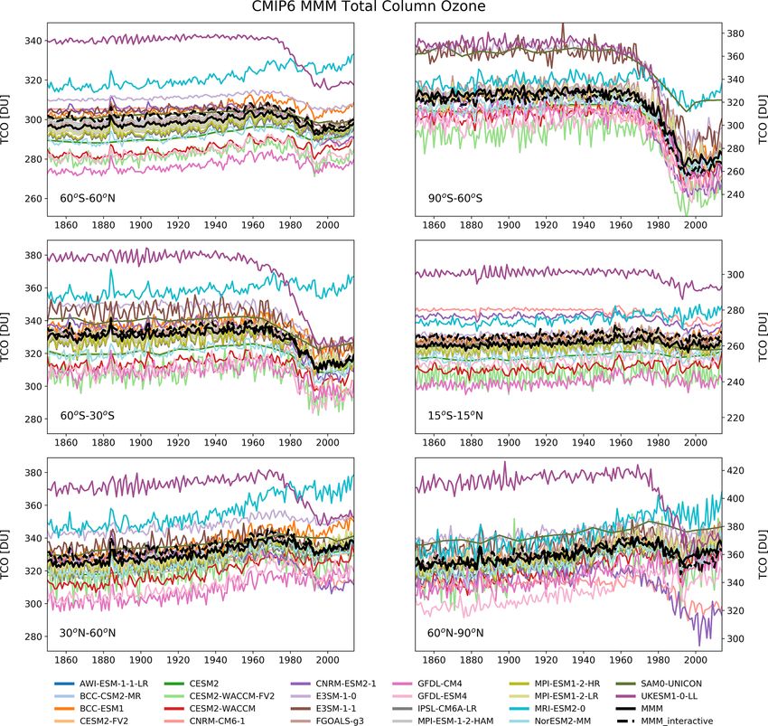
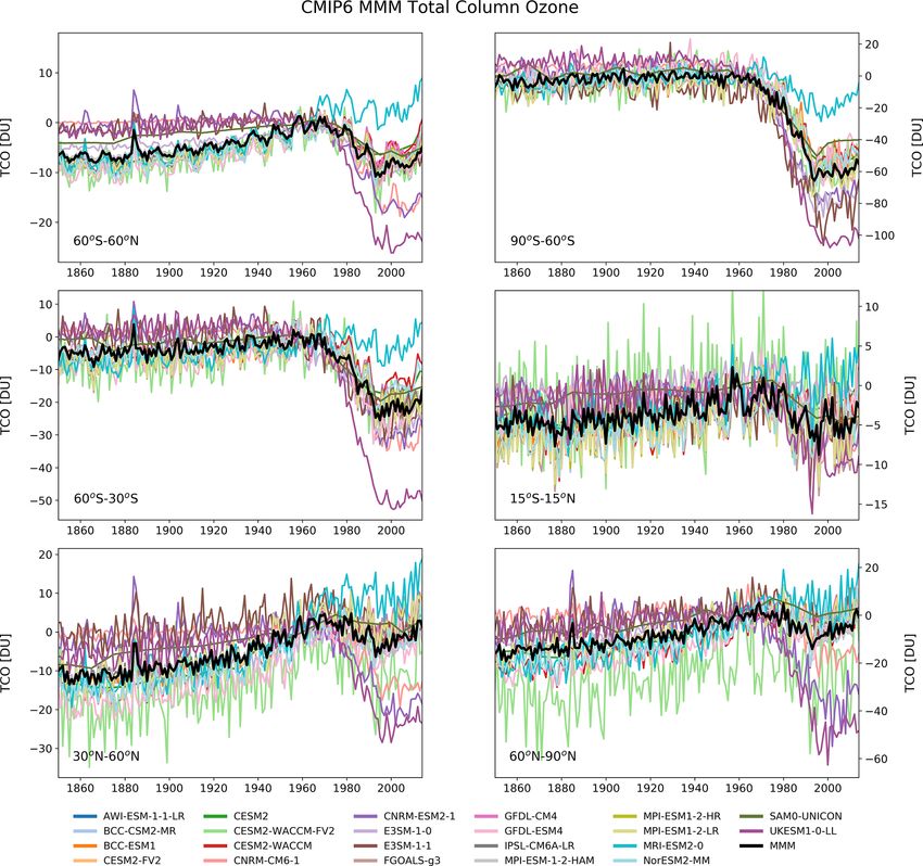
global mean TCO has increased from ∼ 300 DU in 1850 to expansion of the Hadley cell during the SH summer season
∼ 305 DU in 1960, before rapidly declining in the 1970s and (e.g. Thompson and Solomon, 2002; Gillett and Thompson,
1980s following the use and emission of halogenated ozone- 2003; McLandress et al., 2010; Son et al., 2010; Polvani
depleting substances (ODSs). TCO is projected to return to et al., 2011; Braesicke et al.; 2013, Keeble et al., 2014; Mor-
1960s values by the middle of the 21st century under the genstern et al., 2018). In contrast, while no long-term trend
SSP2-4.5, SSP3-7.0, SSP4-3.4, SSP4-6.0, and SSP5-8.5 sce- in stratospheric water vapour has been established (Scherer
narios, and under the SSP3-7.0 and SSP5-8.5 scenarios TCO et al., 2008; Hurst et al., 2011; Hegglin et al., 2014), large
values are projected to be ∼ 10 DU higher than the 1960s decadal variations have been suggested to affect surface tem-
values by 2100. However, under the SSP1-1.9 and SSP1-1.6 peratures (e.g. Solomon et al., 2010). Given these climate
scenarios, TCO is not projected to return to the 1960s values impacts, it is important to understand the drivers of strato-
despite reductions in halogenated ODSs due to decreases in spheric ozone and water vapour and to distinguish long-term
tropospheric ozone mixing ratios. This global pattern is sim- trends from interannual and decadal variability.
ilar to regional patterns, except in the tropics where TCO un- The Intergovernmental Panel on Climate Change (IPCC)
der most scenarios is not projected to return to 1960s values, Fifth Assessment Report (AR5) highlights tropospheric
either through reductions in tropospheric ozone under SSP1- ozone as the third most important anthropogenic green-
1.9 and SSP1-2.6, or through reductions in lower strato- house gas (GHG) with a global mean radiative forcing of
spheric ozone resulting from an acceleration of the Brewer– 0.35 ± 0.2 W m−2 , while stratospheric water vapour changes
Dobson circulation under other Shared Socioeconomic Path- resulting from CH4 oxidation exert a global mean radia-
ways (SSPs). In contrast to TCO, there is poorer agreement tive forcing of 0.07 ± 0.05 W m−2 (Hansen et al., 2005;
between the CMIP6 multi-model mean and observed lower IPCC, 2007, 2013). The primary contributor to the radiative
stratospheric water vapour mixing ratios, with the CMIP6 forcing estimate for ozone is increased tropospheric ozone
multi-model mean underestimating observed water vapour (0.4 ± 0.2 W m−2 ), while recent depletion of stratospheric
mixing ratios by ∼ 0.5 ppmv at 70 hPa. CMIP6 multi-model ozone due to the use and emission of halogenated ODSs,
mean stratospheric water vapour mixing ratios in the tropical compounded with impacts on ozone of increasing CO2 , CH4 ,
lower stratosphere have increased by ∼ 0.5 ppmv from the and N2 O, has resulted in a weakly negative radiative forcing
pre-industrial to the present-day period and are projected to (−0.05 ± 0.1 W m−2 ). Recently, Checa-Garcia et al. (2018a)
increase further by the end of the 21st century. The largest in- estimated ozone radiative forcing using the ozone forcing
creases (∼ 2 ppmv) are simulated under the future scenarios dataset that was developed for the Coupled Model Inter-
with the highest assumed forcing pathway (e.g. SSP5-8.5). comparison Project phase 6 (CMIP6; Eyring et al., 2016)
Tropical lower stratospheric water vapour, and to a lesser and calculated values of 0.28 W m−2 , which, while consistent
extent TCO, shows large variations following explosive vol- with the IPCC-AR5 estimate calculated using model sim-
canic eruptions. ulations, represents an increase of ∼ 80 % compared to the
CMIP5 ozone forcing dataset (Cionni et al., 2011; Stevenson
et al., 2013). The relative uncertainties in radiative forcing
estimates for both stratospheric ozone and water vapour are
1 Introduction large due to the challenges in constraining the concentrations
of both during the pre-satellite era. As a result, the current
Stratospheric ozone and water vapour are key components of radiative forcing estimates rely on ozone and water vapour
the Earth system, and past changes in both have had impor- fields derived from simulations performed by global climate
Atmos. Chem. Phys., 21, 5015–5061, 2021 https://doi.org/10.5194/acp-21-5015-2021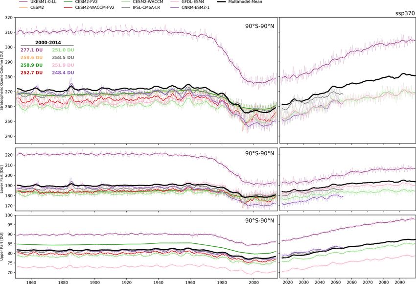
J. Keeble et al.: Evaluating stratospheric ozone and water vapour changes                                                     5017

models and Earth system models. However, models use dif-             Stratospheric water vapour concentrations are determined
ferent radiation schemes and model (in the case of models        predominantly through a combination of the dehydration
with interactive chemistry scheme) or prescribe (in the case     air masses experience as they pass through the tropi-
of models without interactive chemistry schemes) ozone dif-      cal tropopause cold point (Brewer, 1949; Fueglistaler and
ferently, further contributing to the uncertainty estimates.     Haynes, 2005) and in situ production from CH4 oxidation
   Stratospheric ozone concentrations are determined by          (Brasseur and Solomon, 1984; Jones et al., 1986; LeTexier
a balance between production and destruction of ozone            et al., 1988). Direct injections by convective overshooting
through gas-phase chemical reactions and transport (e.g.         (Dessler et al., 2016) or following volcanic eruptions (Mur-
Brewer and Wilson, 1968). Gas-phase ozone chemistry con-         cray et al., 1981; Sioris et al., 2016) are also sources of strato-
sists of sets of oxygen only photochemical reactions first       spheric water vapour.
described by Chapman (1930), alongside ozone destroy-                Observations of stratospheric water vapour show an in-
ing catalytic cycles involving chlorine, nitrogen, hydrogen,     crease during the late 20th century (e.g. Rosenlof et al., 2001;
and bromine radical species (e.g. Bates and Nicolet, 1950;       Scherer et al., 2008; Hurst et al., 2011), followed by a sudden
Crutzen, 1970; Johnston, 1971; Molina and Rowland, 1974;         decrease of ∼ 10 % after 2000 (e.g. Solomon et al., 2010).
Stolarski and Cicerone, 1974). Heterogeneous processes play      Virtually all models project increases in stratospheric wa-
a major role in determining ozone abundances in the polar        ter vapour concentrations under increased CO2 (e.g. Get-
lower stratosphere (e.g. Solomon, 1999) and following large      telman et al., 2010; Banerjee et al., 2019). Projected in-
volcanic eruptions (e.g. Solomon et al., 1996; Telford et al.,   creases over the course of the 21st century occur due to the
2009).                                                           predominant effect of increases in upper tropospheric tem-
   Changes in anthropogenic emissions of halogenated             peratures, offset in part by the effects of a strengthening
ODSs, N2 O, CH4 , CO2 , and other GHGs during the 21st           BDC (Dessler et al., 2013; Smalley et al., 2017), with ad-
century are expected to perturb these chemical cycles either     ditional impacts from future CH4 emissions (Eyring et al.,
directly through their role as source gases or by changing       2010; Gettelman et al., 2010). Eyring et al. (2010) calculate
stratospheric temperatures and dynamics (Eyring et al., 2010;    a mean increase of 0.5–1 ppmv per century in stratospheric
Keeble et al., 2017). Following the implementation of the        water vapour concentrations for models contributing to the
Montreal Protocol and its subsequent amendments, strato-         Chemistry-Climate Model Validation (CCMVal) intercom-
spheric concentrations of inorganic chlorine and bromine         parison project, although agreement between models on the
levelled off in the mid-1990s and are now in decline (Mäder      absolute increase is poor.
et al., 2010; WMO, 2018), which has led to early signs of            To advance our understanding of long-term changes to a
recovery of stratospheric ozone (Keeble et al., 2018; Weber      number of components of the Earth system, including strato-
et al., 2018; WMO 2018) and the detection of statistically ro-   spheric ozone and water vapour, the CMIP panel, operating
bust positive trends in September Antarctic ozone (Solomon       under the auspices of the Working Group on Coupled Mod-
et al., 2016). Total column ozone in the midlatitudes and high   elling (WGCM) of the World Climate Research Programme
latitudes is projected to return to pre-1980 values during the   (WCRP), has defined a suite of climate model experiments,
coming decades (Eyring et al., 2013; Dhomse et al., 2018;        which together form CMIP6 (Eyring et al., 2016). Between
WMO, 2018). Future emissions of CH4 and N2 O, which              the previous phase (CMIP5; Taylor et al., 2012) and CMIP6,
are not regulated in the same way as halogenated ODSs,           there has been further development of existing models, new
are associated with greater uncertainty and future concen-       models have joined and a new set of future scenarios, the
trations of HOx (H, OH, HO2 ), and NOx (NO, NO2 ) rad-           Shared Socioeconomic Pathways (SSPs; Riahi et al., 2017)
icals are highly sensitive to assumptions made about their       that are used in climate projections by CMIP6 models as
future emissions. Additionally, increases in GHG concentra-      part of the Scenario Model Intercomparison Project (Scenar-
tions are expected to lead to an acceleration of the Brewer–     ioMIP; O’Neill et al., 2014), have been established. Earth
Dobson circulation (BDC; Butchart et al., 2006, 2010; Shep-      system models have been further developed with improved
herd and McLandress, 2011; Hardiman et al., 2014; Palmeiro       physical parameterizations and some have added additional
et al., 2014), which may affect ozone concentrations directly    Earth system components (e.g. atmospheric chemistry, nitro-
through transport (e.g. Plumb, 1996; Avallone and Prather,       gen cycle, ice sheets). As a result of this advancement in
1996) and by influencing the chemical lifetimes of Cly , NOy ,   model complexity, the CMIP6 multi-model ensemble pro-
and HOx source gases (e.g. Revell et al., 2012; Meul et al.,     vides an opportunity to re-assess past and projected future
2014). However, recent research (Polvani et al., 2018, 2019)     stratospheric ozone and water vapour changes. In this study,
has shown, using model simulations, that stratospheric ozone     we evaluate these changes against observations over the last
depletion caused by increasing ODSs may have accounted           three decades and examine long-term changes in these quan-
for around half of the acceleration of the BDC in recent         tities from 1850 to 2100 under the SSP scenarios. Section 2
decades. As concentrations of ODSs decline, stratospheric        describes the simulations and models used in this study, with
ozone recovery may offset, at least in part, future changes to   a focus on the treatment of stratospheric ozone and water
the speed of the BDC resulting from GHG changes.                 vapour. Long-term changes in ozone and water vapour are

https://doi.org/10.5194/acp-21-5015-2021                                           Atmos. Chem. Phys., 21, 5015–5061, 2021
5018                                             J. Keeble et al.: Evaluating stratospheric ozone and water vapour changes

evaluated in Sects. 3 and 4, respectively, and implications are    dataset (except in the case of CESM2, CESM2-FV2, and
discussed in Sect. 5. Our results inform future studies that use   NorESM2, which prescribe ozone values from simulations
CMIP6 simulations to investigate stratospheric composition         performed with the CESM2-WACCM model). Relevant
changes and associated impacts.                                    details of each model are provided below, and a summary is
                                                                   provided in Table 1.
                                                                      The CMIP6 ozone dataset (Checa-Garcia, 2018b) is de-
2     Models and simulations                                       signed to be used by those models without interactive chem-
                                                                   istry and was created using a different approach from the
This study evaluates long-term ozone and water vapour              previous CMIP5 ozone database (Cionni et al., 2011). The
changes in 22 models which have performed the CMIP his-            CMIP5 dataset was based on stratospheric ozone values from
torical simulation and a subset of which have performed Sce-       a combination of model and observational datasets between
narioMIP simulations. The treatment of stratospheric chem-         the 1970s and 2011, and extended into the past and future
istry varies significantly across the models evaluated in this     based on assumptions of changes to stratospheric chlorine
study. We evaluate all models which have produced ozone            and the 11-year solar cycle. Tropospheric ozone values were
and water vapour output, regardless of the complexity of the       based on a mean field of two models with interactive chem-
stratospheric chemistry used, as these models may be used in       istry. In contrast, the CMIP6 ozone dataset was created us-
other studies to diagnose the impacts of stratospheric com-        ing simulations from the CMAM and CESM-WACCM mod-
position changes on radiative forcing and/or regional climate      els, which both performed the REF-C2 simulation as part of
change. In this section, the models and simulations used in        the Chemistry-Climate Model Initiative (Eyring, et al., 2013;
the subsequent analysis sections are described, along with the     Morgenstern et al., 2017). As a result, the CMIP6 dataset
observational datasets used for evaluation. Several of the fig-    provides a full three-dimensional field of ozone mixing ra-
ures were created with the Earth System Model Evaluation           tios created using a single, consistent approach for both the
Tool (ESMValTool) version 2.0 (Eyring et al., 2020; Righi          stratosphere and troposphere, extending from pre-industrial
et al., 2020), a diagnostic and performance metric tool for        times to the present day, and until the end of the 21st century
enhanced and more comprehensive Earth system model eval-           following the different SSP scenarios (O’Neill et al., 2014).
uation in CMIP.                                                    However, as the CMIP6 dataset uses values from model sim-
                                                                   ulations, it has biases with respect to observations and uncer-
2.1    Models                                                      tainties associated with the projections of stratospheric ozone
                                                                   beyond the period observations exist for, both from the pre-
At the time of the preparation of this paper, 22 models (AWI-      industrial period to the start of the observational record and
ESM-1-1-LR, BCC-CSM2-MR, BCC-ESM1, CESM2,                          from the present day to the end of the 21st century under the
CESM2-FV2, CESM2-WACCM, CESM2-WACCM-FV2,                           different SSP scenarios. More details on the CMIP6 ozone
CNRM-CM6-1, CNRM-ESM2-1, E3SM-1-0, E3SM-1-1,                       dataset can be found in Checa-Garcia (2018b).
FGOALS-g3, GFDL-CM4, GFDL-ESM4, IPSL-CM6A-LR,                         AWI-ESM-1-1-LR. The Alfred Wegener Institute
MPI-ESM-1-2-HAM, MPI-ESM1-2-HR, MPI-ESM1-2-                        Earth System Model (AWI-ESM) is the global coupled
LR, MRI-ESM2-0, NorESM2-MM, SAM0-UNICON,                           atmosphere–land–ocean–sea ice model AWI Climate Model
and UKESM1-0-LL) have provided ozone mixing ratios                 (AWI-CM; Semmler et al., 2020) extended by a dynamic
and 18 models (AWI-ESM-1-1-LR, BCC-CSM2-MR,                        land cover change model. Atmosphere and land are repre-
BCC-ESM1, CESM2, CESM2-FV2, CESM2-WACCM,                           sented by a 1.85◦ × 1.85◦ horizontal resolution configuration
CESM2-WACCM-FV2, CNRM-CM6-1, CNRM-ESM2-1,                          of ECHAM6 (47 vertical levels up to 0.01 hPa ∼ 80 km;
E3SM-1-1, GFDL-CM4, IPSL-CM6A-LR, MPI-ESM-1-2-                     Stevens et al., 2013), which includes a land component (JS-
HAM, MPI-ESM1-2-HR, MPI-ESM1-2-LR, MRI-ESM2-0,                     BACH; Reick et al., 2013). The ocean is represented by the
NorESM2-MM, and UKESM1-0-LL) have provided wa-                     sea ice–ocean model FESOM1.4 (Wang et al., 2014), which
ter vapour as diagnostics. Of the 22 models analysed               runs on an irregular grid with a nominal resolution of 150 km
in this study, six (CESM2-WACCM, CESM2-WACCM-                      (smallest grid size 25 km). Tropospheric and stratospheric
FV2, CNRM-ESM2-1, GFDL-ESM4, MRI-ESM2-0, and                       ozone is prescribed from the CMIP6 dataset (Checa-Garcia
UKESM1-0-LL) use interactive stratospheric chemistry               et al., 2018a). GHG concentrations including CO2 , CH4 ,
schemes, while three (CNRM-CM6-1, E3SM-1-0, and                    N2 O, and chlorofluorocarbons (CFCs) are prescribed after
E3SM-1-1) use a simple chemistry scheme. The remaining             Meinshausen et al. (2017). Methane oxidation and photolysis
13 (AWI-ESM-1-1-LR, BCC-CSM2-MR, BCC-ESM1,                         of water vapour are parameterized for the stratosphere and
CESM2, CESM2-FV2, FGOALS-g3, GFDL-CM4, IPSL-                       mesosphere (further information in Sect. 2.1.2 of Schmidt
CM6A-LR,         MPI-ESM-1-2-HAM,           MPI-ESM1-2-HR,         et al., 2013, and references therein).
MPI-ESM1-2-LR, NorESM2-MM, and SAM0-UNICON)                           BCC-CSM2-MR. The BCC-CSM2-MR model, devel-
do not include an interactive chemistry scheme and instead         oped by the Beijing Climate Center, is a coupled ocean–
prescribe stratospheric ozone according to the CMIP6 ozone         atmosphere model. Ozone in the stratosphere and tropo-

Atmos. Chem. Phys., 21, 5015–5061, 2021                                             https://doi.org/10.5194/acp-21-5015-2021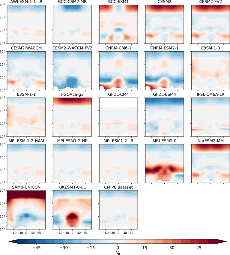
J. Keeble et al.: Evaluating stratospheric ozone and water vapour changes                                                                                      5019

Table 1. Overview of models and data available at the time this paper was prepared, providing model name, horizontal and vertical resolution,
the stratospheric chemistry scheme used, the simulations each model performed, and the Earth System Grid Federation (ESGF) reference
for the model datasets. For the stratospheric chemistry scheme, models use either interactive chemistry (denoting fully coupled, complex
chemistry schemes), simplified online schemes (denoting simple, linear schemes), or prescribed stratospheric ozone fields. Most models
prescribing stratospheric ozone use the CMIP6 dataset (Checa-Garcia, 2018b), except CESM2, CESM2-FV2, and NorESM2, which prescribe
ozone values from simulations performed with the CESM2-WACCM model. Numbers in parentheses in the ozone and water vapour columns
give the number of ensemble members that performed each of the listed simulations.

  Model              Resolution                                                 Stratospheric       Ozone             Water vapour      Datasets
                                                                                chemistry
  AWI-ESM-1-1-LR     192 × 96 longitude–latitude; 47 levels; top level 80 km    Prescribed          Historical (1)    Historical (1)    Danek et al. (2020)
                                                                                (CMIP6 dataset)
  BCC-CSM2-MR        320 × 160 longitude–latitude; 46 levels; top level         Prescribed          Historical (3)    Historical (3)    Wu et al. (2019a)
                     1.46 hPa                                                   (CMIP6 dataset)     SSP1-2.6 (1)      SSP1-2.6 (1)      Xin et al. (2019)
                                                                                                    SSP2-4.5 (1)      SSP2-4.5 (1)
                                                                                                    SSP3-7.0 (1)      SSP3-7.0 (1)
                                                                                                    SSP5-8.5 (1)      SSP5-8.5 (1)
  BCC-ESM1           128 × 64 longitude–latitude; 26 levels; top level          Prescribed          Historical (3)    Historical (3)    Zhang et al. (2018)
                     2.19 hPa                                                   (CMIP6 dataset)
  CESM2              288 × 192 longitude–latitude; 32 levels; top level         Prescribed          Historical (11)   Historical (11)   Danabasoglu (2019a)
                     2.25 hPa                                                   (other)             SSP1-2.6 (1)      –                 Danabasoglu (2019b)
                                                                                                    SSP2-4.5 (1)      SSP2-4.5 (1)
                                                                                                    SSP3-7.0 (2)      –
                                                                                                    SSP5-8.5 (2)      –
  CESM2-FV2          144 × 96 longitude–latitude; 32 levels; top level          Prescribed          Historical (1)    Historical (1)    Danabasoglu (2019c)
                     2.25 hPa                                                   (other)

  CESM2-WACCM        144 × 96 longitude–latitude; 70 levels; top level          Interactive         Historical (3)    Historical (3)    Danabasoglu (2019d)
                     4.5 × 10⁻⁶ hPa                                             chemistry           SSP1-2.6 (1)      –                 Danabasoglu (2019e)
                                                                                                    SSP2-4.5 (1)      SSP2-4.5 (1)
                                                                                                    SSP3-7.0 (3)      –
                                                                                                    SSP5-8.5 (1)      –
  CESM2-WACCM-       144 × 96 longitude–latitude; 70 levels; top level          Interactive         Historical (1)    Historical (1)    Danabasoglu (2019f)
  FV2                4.5 × 10⁻⁶ hPa                                             chemistry
  CNRM-CM6-1         T127; Gaussian reduced with 24 572 grid points in to-      Simplified online   Historical (19)   Historical (19)   Voldoire (2018)
                     tal distributed over 128 latitude circles (with 256 grid   scheme              SSP1-2.6 (6)      SSP1-2.6 (6)      Voldoire (2019)
                     points per latitude circle between 30◦ N and 30◦ S re-                         SSP2-4.5 (6)      SSP2-4.5 (6)
                     ducing to 20 grid points per latitude circle at 88.9◦ N                        SSP3-7.0 (6)      SSP3-7.0 (6)
                     and 88.9◦ S); 91 levels; top level 78.4 km                                     SSP5-8.5 (6)      SSP5-8.5 (6)
  CNRM-ESM2-1        T127; Gaussian reduced with 24 572 grid points in to-      Interactive         Historical (5)    Historical (5)    Séférian (2018)
                     tal distributed over 128 latitude circles (with 256 grid   chemistry           SSP1-1.9 (5)      SSP1-1.9 (5)      Séférian (2019)
                     points per latitude circle between 30◦ N and 30◦ S re-                         SSP1-2.6 (5)      –
                     ducing to 20 grid points per latitude circle at 88.9◦ N                        SSP2-4.5 (5)      SSP2-4.5 (5)
                     and 88.9◦ S); 91 levels; top level 78.4 km                                     SSP3-7.0 (5)      SSP3-7.0 (5)
                                                                                                    SSP4-3.4 (5)      SSP4-3.4 (5)
                                                                                                    SSP4-6.0 (5)      SSP4-6.0 (5)
                                                                                                    SSP5-8.5 (5)      SSP5-8.5 (5)
  E3SM-1-0           Cubed-sphere spectral-element grid; 5400 elements          Simplified online   Historical (5)    –                 Bader et al. (2019a)
                     with p = 3; 1◦ average grid spacing; 90 × 90 × 6           scheme
                     longitude–latitude–cube face; 72 levels; top level
                     0.1 hPa
  E3SM-1-1           Cubed-sphere spectral-element grid; 5400 elements          Simplified online   Historical (1)    Historical (1)    Bader et al. (2019b)
                     with p = 3; 1◦ average grid spacing; 90 × 90 × 6           scheme
                     longitude–latitude–cube face; 72 levels; top level
                     0.1 hPa
  FGOALS-g3          180 × 80 longitude–latitude; 26 levels; top level          Prescribed          Historical (3)    –                 Li (2019)
                     2.19 hPa                                                   (CMIP6 dataset)     SSP1-2.6 (1)
                                                                                                    SSP3-7.0 (1)
                                                                                                    SSP5-8.5 (1)
  GFDL-CM4           360 × 180 longitude–latitude; 33 levels; top level 1 hPa   Prescribed          Historical (1)    Historical (1)    Guo et al. (2018a)
                                                                                (CMIP6 dataset)     SSP2-4.5 (1)      SSP2-4.5 (1)      Guo et al. (2018b)
                                                                                                    SSP5-8.5 (1)      SSP5-8.5 (1)

https://doi.org/10.5194/acp-21-5015-2021                                                                 Atmos. Chem. Phys., 21, 5015–5061, 2021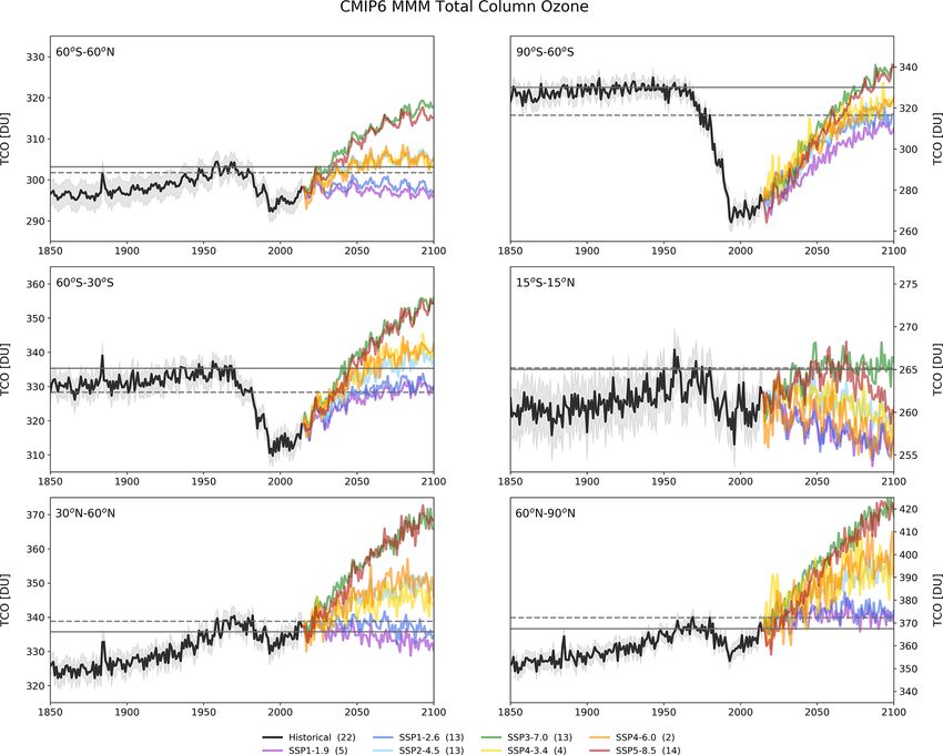
5020                                                          J. Keeble et al.: Evaluating stratospheric ozone and water vapour changes

Table 1. Continued.

  Model               Resolution                                                 Stratospheric     Ozone             Water vapour      Datasets
                                                                                 chemistry
  GFDL-ESM4           360 × 180 longitude–latitude; 49 levels; top level 1 Pa    Interactive       Historical (1)    Historical (1)    Krasting et al. (2018)
                                                                                 chemistry         SSP1-1.9 (1)      –                 John et al. (2018)
                                                                                                   SSP1-2.6 (1)      SSP1-2.6 (1)
                                                                                                   SSP2-4.5 (1)      –
                                                                                                   SSP3-7.0 (1)      SSP3-7.0 (1)
                                                                                                   SSP5-8.5 (1)      –
  IPSL-CM6A-LR        144 × 143 longitude–latitude; 79 levels; top level 80 km   Prescribed        Historical (20)   Historical (20)   Boucher et al. (2018)
                                                                                 (CMIP6 dataset)   SSP1-1.9 (1)      SSP1-1.9 (1)      Boucher et al. (2019)
                                                                                                   SSP1-2.6 (3)      SSP1-2.6 (3)
                                                                                                   SSP2-4.5 (2)      SSP2-4.5 (2)
                                                                                                   SSP3-7.0 (10)     SSP3-7.0 (10)
                                                                                                   SSP4-3.4 (1)      SSP4-3.4 (1)
                                                                                                   –                 SSP4-6.0 (1)
                                                                                                   SSP5-8.5 (1)      SSP5-8.5 (1)
  MPI-ESM-1-2-        192 × 96 longitude–latitude; 47 levels; top level          Prescribed        Historical (2)    Historical (2)    Neubauer et al. (2019a)
  HAM                 0.01 hPa                                                   (CMIP6 dataset)
  MPI-ESM1-2-HR       384 × 192 longitude–latitude; 95 levels; top level         Prescribed        Historical (10)   Historical (10)   Jungclaus et al. (2019)
                      0.01 hPa                                                   (CMIP6 dataset)   SSP1-2.6 (2)      –
                                                                                                   SSP2-4.5 (2)      SSP2-4.5 (2)
                                                                                                   SSP3-7.0 (10)     –
                                                                                                   SSP5-8.5 (2)      –
  MPI-ESM1-2-LR       192 × 96 longitude–latitude; 47 levels; top level          Prescribed        Historical (10)   Historical (10)   Wieners et al. (2019)
                      0.01 hPa                                                   (CMIP6 dataset)   SSP1-2.6 (3)      –
                                                                                                   SSP2-4.5 (3)      SSP2-4.5 (3)
                                                                                                   SSP3-7.0 (3)      –
                                                                                                   SSP5-8.5 (3)      –
  MRI-ESM2-0          192 × 96 longitude–latitude; 80 levels; top level          Interactive       Historical (5)    Historical (5)    Yukimoto et al. (2019a)
                      0.01 hPa                                                   chemistry         SSP1-1.9 (1)      SSP1-1.9 (1)      Yukimoto et al. (2019b)
                                                                                                   SSP1-2.6 (1)      SSP1-2.6 (1)
                                                                                                   SSP2-4.5 (5)      SSP2-4.5 (5)
                                                                                                   SSP3-7.0 (5)      SSP3-7.0 (5)
                                                                                                   SSP4-3.4 (1)      SSP4-3.4 (1)
                                                                                                   SSP4-6.0 (1)      SSP4-6.0 (1)
                                                                                                   SSP5-8.5 (1)      SSP5-8.5 (1)
  NorESM2-MM          288 × 192; 32 levels; top level 3 hPa                      Prescribed        Historical (1)    Historical (1)    Bentsen et al. (2019)
                                                                                 (other)           SSP1-2.6 (1)      –
                                                                                                   SSP2-4.5 (1)      SSP2-4.5 (1)
                                                                                                   SSP3-7.0 (1)      –
                                                                                                   SSP5-8.5 (1)      –
  SAM0-UNICON         288 × 192 longitude–latitude; 30 levels; top level         Prescribed        Historical (1)    –                 Park and Shin (2019)
                      ∼ 2 hPa                                                    (CMIP6 dataset)
  UKESM1-0-LL         192 × 144 longitude–latitude; 85 levels; top level 85 km   Interactive       Historical (9)    Historical (9)    Tang et al. (2019)
                                                                                 chemistry         SSP1-1.9 (5)      SSP1-1.9 (5)      Good et al. (2019)
                                                                                                   SSP1-2.6 (5)      SSP1-2.6 (5)
                                                                                                   SSP2-4.5 (5)      SSP2-4.5 (5)
                                                                                                   SSP3-7.0 (5)      SSP3-7.0 (5)
                                                                                                   SSP4-3.4 (5)      SSP4-3.4 (5)
                                                                                                   SSP5-8.5 (5)      SSP5-8.5 (5)

sphere is prescribed using monthly mean time-varying grid-                               BCC-ESM1. The BCC-ESM1 model, developed by the
ded data from the CMIP6 dataset. Other GHG concentra-                                 Beijing Climate Center, is a fully coupled global climate–
tions including CO2 , N2 O, CH4 , CFC-11, and CFC-12 are                              chemistry–aerosol model. Tropospheric ozone is modelled
monthly zonal mean values using the CMIP6 datasets (Mein-                             interactively using the Model for OZone and Related chemi-
shausen et al., 2017, 2020). Stratospheric water vapour con-                          cal Tracers version 2 (MOZART2) chemistry scheme, while
centrations are prognostic values calculated in a similar way                         stratospheric ozone is prescribed to the zonally averaged,
to those in the troposphere. A full description and evalua-                           monthly mean values from 1850 to 2014 derived from the
tion of the BCC-CSM2-MR model are provided by Wu et al.                               CMIP6 data package in the top two model layers and re-
(2020).                                                                               laxed towards the CMIP6 dataset between these layers and
                                                                                      the tropopause. GHG concentrations including CH4 , N2 O,

Atmos. Chem. Phys., 21, 5015–5061, 2021                                                                  https://doi.org/10.5194/acp-21-5015-2021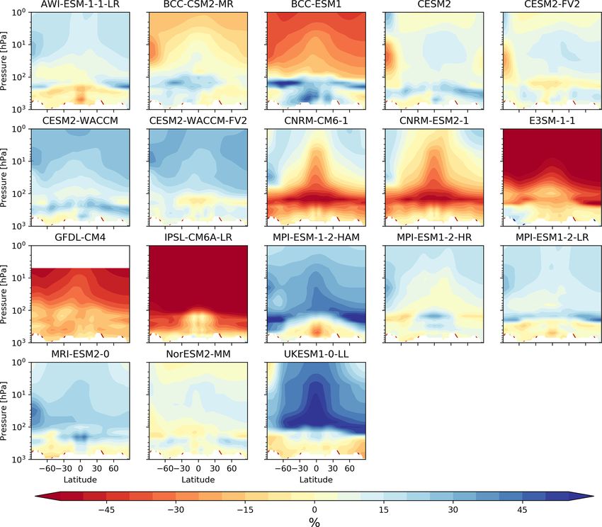
J. Keeble et al.: Evaluating stratospheric ozone and water vapour changes                                                5021

CO2 , CFC-11, and CFC-12 are prescribed using CMIP6 his-         ClOx , and BrOx chemical families, CH4 and its degradation
torical forcing data as suggested in the AerChemMIP pro-         products, N2 O (major source of NOx ), H2 O (major source
tocol (Collins et al., 2017). Stratospheric water vapour is a    of HOx ), plus various natural and anthropogenic precursors
prognostic variable without any special treatment of CH4 ox-     of the ClOx and BrOx families. The TSMLT mechanism
idation. A full description and evaluation of the BCC-ESM1       also includes primary non-methane hydrocarbons and re-
model are provided by Wu et al. (2020b).                         lated oxygenated organic compounds, and two very short-
   CESM2. The Community Earth System Model version 2             lived halogens (CHBr3 and CH2 Br2 ) which add an additional
(CESM2) is the latest generation of the coupled climate–         ∼ 5 ppt of inorganic bromine to the stratosphere. WACCM6
Earth system models developed as a collaborative effort be-      features a new prognostic representation of stratospheric
tween scientists, software engineers, and students from the      aerosols based on sulfur emissions from volcanoes and other
National Center for Atmospheric Research (NCAR), univer-         sources, and a new detailed representation of secondary or-
sities, and other research institutions. CESM2(CAM6) uses        ganic aerosols (SOAs) based on the volatility basis set ap-
the Community Atmosphere Model version 6 as its atmo-            proach from major anthropogenic and biogenic volatile or-
sphere component, which has 32 vertical levels from the          ganic compound precursors. A full description of WACCM6
surface to 3.6 hPa (about 40 km) and a horizontal resolution     is provided by Gettelman et al. (2019).
of 1.25◦ longitude by 0.95◦ latitude, and limited interactive       CESM2-WACCM-FV2. The CESM2-WACCM-FV2
chemistry for tropospheric aerosols. GHG concentrations in-      model is based on CESM2-WACCM but with a reduced
cluding CH4 , N2 O, CO2 , CFC-11eq, and CFC-12 are pre-          horizontal resolution for the atmosphere and land compo-
scribed using CMIP6 historical forcing data. CESM2 uses          nents of 2.5◦ longitude by 1.8◦ latitude. The three tuning
datasets derived from previous runs of CESM2-WACCM6,             parameters adjusted for CESM2-FV2 were set consistently
which includes interactive chemistry, for tropospheric oxi-      for CESM2-WACCM-FV2. The dust emission factor was
dants (O3 , OH, NO3 , and HO2 ; 3-D monthly means), strato-      also changed from 0.7 to 0.26. In addition, several WACCM-
spheric water vapour production from CH4 oxidation (3-           specific adjustments were made for model consistency at
D monthly means), stratospheric aerosol (zonal 5 d means),       FV2 resolution. The efficiency associated with convective
and O3 for use in radiative transfer calculations (zonal 5 d     gravity waves from the Beres scheme for deep convection
means). A full description and evaluation of the CESM2           (effgw_beres_dp) was changed from 0.5 to 0.1. The fron-
model are provided by Danabasoglu et al. (2020).                 togenesis function critical threshold (frontgfc) was changed
   CESM2-FV2. The Community Earth System Model ver-              from 3.0 to 1.25. The background source strength used for
sion 2 – finite volume 2◦ (CESM2-FV2) is based on CESM2          waves from frontogenesis (taubgnd) was changed from 2.5
but with a reduced horizontal resolution for the atmosphere      to 1.5. The multiplication factor applied to the lightning
and land components of 2.5◦ longitude by 1.8◦ latitude.          NOx production (lght_no_prd_factor) was changed from
CESM2-FV2 uses the same finite volume (FV) dynamical             1.5 to 1.0. Finally, the quasi-biennial oscillation (QBO) is
core as CESM2. Three tuning parameters were adjusted to          nudged in CESM2-WACCM-FV2, while it is self-generating
maintain consistency with CESM2. To maintain the top-of-         in CESM2-WACCM.
atmosphere energy balance, the clubb_gamma_coef param-              CNRM-CM6-1. The CNRM-CM6-1 model, developed by
eter, described in Danabasoglu et al. (2020), was reduced        the Centre National de Recherches Météorologiques, is a
from 0.308 to 0.280, and the autoconversion size threshold       global climate model which uses a linearized scheme to
from cloud ice to snow (micro_mg_dcs) was decreased from         model stratospheric ozone, in which ozone mixing ratios are
500 to 200 µm. To maintain sea salt aerosol burdens consis-      treated as a prognostic variable with photochemical produc-
tent with observations, the emission factor for sea salt was     tion and loss rates computed from its associated Earth system
changed from 1.0 to 1.1.                                         model (CNRM-ESM2-1). The model does not include inter-
   CESM2-WACCM. The CESM2-WACCM model uses the                   active tropospheric ozone chemistry. Details of the lineariza-
Whole Atmosphere Community Climate Model version 6               tion of the net photochemical production in the ozone conti-
(WACCM6) as its atmosphere component. WACCM6 has                 nuity equation are provided by Michou et al. (2020). Tropo-
70 vertical levels from the surface to 6 × 0−6 hPa (about        spheric ozone mixing ratios are not calculated interactively
140 km), a horizontal resolution of 1.25◦ longitude by           and are instead prescribed from the CMIP6 dataset. Methane
0.95◦ latitude. WACCM6 features a comprehensive chem-            oxidation is parameterized throughout the model domain by
istry mechanism with a description of the troposphere, strato-   the introduction of a simple relaxation of the upper strato-
sphere, mesosphere, and lower thermosphere (TSMLT), in-          spheric moisture source due to methane oxidation (Untch
cluding 231 species, 150 photolysis reactions, 403 gas-          and Simmons, 1999). A sink representing photolysis in the
phase reactions, 13 tropospheric heterogeneous reactions,        mesosphere is also included. A full description and evalua-
and 17 stratospheric heterogeneous reactions. The photolytic     tion of the CNRM-CM6-1 model are provided by Voldoire
calculations are based on both inline chemical modules and       et al. (2019).
a lookup table approach. The chemical species within the            CNRM-ESM2-1. The CNRM-ESM2-1 model, developed
TSMLT mechanism include the extended Ox , NOx , HOx ,            by the Centre National de Recherches Météorologiques, is

https://doi.org/10.5194/acp-21-5015-2021                                         Atmos. Chem. Phys., 21, 5015–5061, 2021
5022                                             J. Keeble et al.: Evaluating stratospheric ozone and water vapour changes

a coupled Earth system model. The chemistry scheme of              description and evaluation of the GFDL-CM4 model are pro-
CNRM-ESM2-1 is an online scheme in which the chem-                 vided by Held et al. (2019).
istry routines are part of the physics of the atmospheric cli-        GFDL-ESM4. The GFDL-ESM4 model, developed by the
mate model and are called at each time step (Michou et al.,        National Oceanic and Atmospheric Administration’s Geo-
2011). The scheme considers 168 chemical reactions, among          physical Fluid Dynamics Laboratory, is a fully coupled
which 39 are photolysis reactions and 9 represent the hetero-      chemistry–climate model. Stratospheric ozone is calculated
geneous chemistry. This scheme is applied in the whole at-         using an interactive tropospheric and stratospheric gas-phase
mosphere above 560 hPa but does not include tropospheric           and aerosol chemistry scheme. The atmospheric component
ozone non-methane hydrocarbon chemistry. The 3-D con-              (AM4.1) includes 56 prognostic (transported) tracers and 36
centrations of several trace gases interact with the atmo-         diagnostic (non-transported) chemical tracers, with 43 pho-
spheric radiative code at each call of the radiation scheme.       tolysis reactions, 190 gas-phase kinetic reactions, and 15 het-
In addition to the non-orographic gravity wave drag param-         erogeneous reactions. The tropospheric chemistry includes
eterization, a sponge layer is also used in the upper levels to    reactions for the NOx –HOx –Ox –CO–CH4 system and oxida-
reduce spurious reflections of vertically propagating waves        tion schemes for other non-methane volatile organic com-
from the model top. This parameterization consists simply of       pounds. The stratospheric chemistry accounts for the ma-
a linear relaxation of the wind towards zero. The linear relax-    jor ozone loss cycles (Ox , HOx , NOx , ClOx , and BrOx ) and
ation is active above 0.03 hPa. A full description and evalua-     heterogeneous reactions on liquid and solid stratospheric
tion of the CNRM-ESM2-1 model are provided by Séférian             aerosols (Austin et al., 2013). Photolysis rates are calcu-
et al. (2019), while an evaluation of the ozone radiative forc-    lated interactively using the FAST-JX version 7.1 code, ac-
ing is detailed in Michou et al. (2020).                           counting for the radiative effects of simulated aerosols and
   E3SM-1-0 and E3SM-1-1. The E3SM-1-0 and E3SM-1-                 clouds. Details on the chemical mechanism will be included
1 models, developed by the US Department of Energy, are            in Horowitz et al. (2020). A full description and evaluation of
coupled Earth system models. They both use a simplified,           the GFDL-ESM4 model are provided by Dunne et al. (2020).
linearized ozone photochemistry scheme to predict strato-             IPSL-CM6A-LR. The IPSL-CM6A-LR model, devel-
spheric ozone changes (Linoz v2; Hsu and Prather, 2009).           oped by the Institut Pierre-Simon Laplace, is a coupled
Stratospheric water vapour does not include a source from          atmosphere–land–ocean–sea ice model. Stratospheric and
methane oxidation. The E3SM-1-1 model simulations dif-             tropospheric ozone is prescribed using the CMIP6 dataset
fer from those of the E3SM-1-0 model primarily by includ-          but implemented so that profiles are stretched in a thin re-
ing active prediction of land and ocean biogeochemistry re-        gion (few kilometres only) around the tropopause, ensuring
sponses to historical increases in atmospheric CO2 . This is       that the tropopause of the ozone climatology and that of the
in contrast to the E3SM-1-0 simulations, which used a pre-         model match. Differences in tropopause heights would lead
scribed phenology for land vegetation and did not simulate         to spurious ozone transport between the upper troposphere
ocean biogeochemistry. The ocean biogeochemistry has no            and lower stratosphere, a region where the corresponding
physical feedbacks in E3SM-1-1, but the land biogeochem-           non-physical radiative impact would be particularly high
istry impacts surface water and energy fluxes, leading to mi-      (e.g. Hardiman et al., 2019). Stratospheric methane oxidation
nor changes in the atmospheric circulation. A full description     is not included in the version of the model evaluated here. A
of the E3SM-1-0 model is provided by Golaz et al. (2019),          full description and evaluation of the IPSL-CM6A-LR model
while a complete description of E3SM-1-1 is provided in            are provided by Boucher et al. (2020).
Burrows et al. (2020).                                                MPI-ESM-1-2-HAM. The MPI-ESM-1-2-HAM model,
   FGOALS-g3. The FGOALS-g3 model, developed by                    developed by the HAMMOZ consortium involving re-
the Chinese Academy of Sciences, is a coupled ocean–               searchers from ETH Zurich (Switzerland), the Center for
atmosphere model. FGOALS-g3 does not include an interac-           Climate Systems Modeling Zurich (Switzerland), the Uni-
tive chemistry module, and ozone is prescribed in the strato-      versity of Oxford (United Kingdom), the Finish Meteoro-
sphere and troposphere following the recommendations by            logical Institute Kuopio (Finland), the Max Planck Institute
CMIP6. Stratospheric water vapour concentrations are prog-         for Meteorology Hamburg (Germany), Forschungszentrum
nostic values calculated in a similar way to those in the tropo-   Jülich (Germany), GEOMAR Helmholtz-Centre for Ocean
sphere. A full description and evaluation of the FGOALS-g3         Research Kiel (Germany), and the Leibniz Institute for Tro-
model are provided by Li et al. (2020).                            pospheric Research (TROPOS) Leipzig (Germany), uses the
   GFDL-CM4. The GFDL-CM4 model, developed by the                  Max Planck Institute (MPI) Earth System Model version 1.2
National Oceanic and Atmospheric Administration’s Geo-             (Mauritsen et al., 2019) as the basic ESM which is coupled to
physical Fluid Dynamics Laboratory, is a coupled ocean–            the aerosol microphysics package Hamburg Aerosol Model
atmosphere model. Ozone is prescribed using the recom-             (HAM) including parameterizations for aerosol–cloud in-
mended CMIP6 dataset throughout the troposphere and                teractions. In ECHAM6-HAM, the atmospheric part of the
stratosphere, while stratospheric water vapour is interactive      model has a spectral core and is run at a horizontal resolu-
but does not include a source from methane oxidation. A full       tion of T63 (approximately 1.875◦ latitude × 1.875◦ longi-

Atmos. Chem. Phys., 21, 5015–5061, 2021                                             https://doi.org/10.5194/acp-21-5015-2021
J. Keeble et al.: Evaluating stratospheric ozone and water vapour changes                                                 5023

tude) and with 47 levels in the vertical domain up to 0.01 hPa   of CESM2-WACCM6. A full description of the NorESM2-
(approximately 80 km). The abundance of ozone in the at-         MM model is provided by Seland et al. (2020).
mosphere is prescribed following the CMIP6 dataset. Water           SAM0-UNICON. The SAM0-UNICON, developed by the
vapour is a prognostic variable including a parameterization     Seoul National University, is a general circulation model
of methane oxidation and photolysis in the stratosphere and      based on the CESM1 model with a unified convection
mesosphere. A full description of the model is provided by       scheme (Park 2014a, b) that replaces shallow and deep con-
Tegen et al. (2019) and Neubauer et al. (2019b).                 vection schemes in CESM1. Stratospheric and tropospheric
   MPI-ESM1-2-HR and MPI-ESM1-2-LR. The MPI Earth                ozone is prescribed as a monthly mean 3-D field, taken
System Model (MPI-ESM) version 1.2, developed by the             from the CMIP6 ozone dataset, with a specified annual cy-
Max Planck Institute for Meteorology in Germany, is a global     cle. Stratospheric water vapour does not include a source
coupled atmosphere–land–ocean–sea ice biogeochemistry            from methane oxidation. A full description of the SAM0-
model. The atmosphere component, ECHAM6, uses spectral           UNICON model is provided by Park et al. (2019).
dynamics with a model top at 0.01 hPa. MPI-ESM is pro-              UKESM1-0-LL. The UKESM1-0-LL model, developed
vided for two configurations (Müller et al., 2018; Maurit-       jointly by the United Kingdom’s Met Office and Natural En-
sen et al., 2019). In the HR configuration, the atmospheric      vironment Research Council, is a fully coupled Earth sys-
longitude–latitude resolution is 0.9375◦ × 0.9375◦ (T127)        tem model. UKESM1-0-LL uses a combined troposphere–
with 95 levels in the vertical; in LR, it is 1.875◦ × 1.875◦     stratosphere chemistry scheme (Archibald et al., 2019),
(T63) with 47 levels. For LR, the land surface uses dynamic      which includes 84 tracers, 199 bimolecular reactions, 25 uni-
land cover change instead of prescribed vegetation maps. For     and termolecular reactions, 59 photolytic reactions, 5 hetero-
both configurations, ozone is prescribed on all levels follow-   geneous reactions, and 3 aqueous-phase reactions for the sul-
ing the CMIP6 recommendations. CH4 , N2 O, CO2 , CFC-11,         fur cycle. As a result, stratospheric ozone and water vapour
and CFC-12 are prescribed using annual global means pro-         are fully interactive. A full description and evaluation of the
vided by CMIP6. Methane oxidation and photolysis of wa-          UKESM1-0-LL model are provided by Sellar et al. (2019).
ter vapour are parameterized for the stratosphere and meso-
sphere (Schmidt et al., 2013, cf. Sect. 2.1.2).                  2.2   Simulations
   MRI-ESM2-0. The MRI-ESM2-0 model, developed by
the Meteorological Research Institute, Japan Meteorological      To evaluate changes in stratospheric ozone and water vapour
Agency, is a fully coupled global climate model which in-        from 1850 to 2100, this study makes use of two types of
cludes interactive chemistry. MRI-ESM2-0’s chemistry com-        simulations performed as part of the wider CMIP6 activity:
ponent is the MRI-CCM2.1 module, which simulates the dis-        the CMIP6 historical simulation (Eyring et al., 2016) and the
tribution and evolution of ozone and other trace gases in the    ScenarioMIP future simulations (O’Neill et al., 2014).
troposphere and middle atmosphere. MRI-CCM2.1 is an up-             The CMIP6 historical simulation runs from 1850 to 2014,
dated version of MRI-CCM2 (Deushi and Shibata, 2011),            in which the models are forced by common datasets based on
which calculates a total of 90 chemical species and 259          observations which include historical changes in short-lived
chemical reactions. MRI-ESM2-0 simulates the stratospheric       species (e.g. NOx , CO, and VOCs) and long-lived GHGs
water vapour interactively with consideration for production     and ODSs (e.g. CO2 , CH4 , N2 O, CFC-11, and CFC-12),
of water vapour from CH4 oxidation. A full description and       global land use, solar forcing, stratospheric aerosols from
evaluation of the MRI-ESM2-0 model are provided by Yuki-         volcanic eruptions, and, for models without ozone chemistry,
moto et al. (2019c).                                             prescribed time-varying ozone concentrations. These simu-
   NorESM2-MM. The second version of the Norwegian               lations are initialized from the pre-industrial control (piCon-
Earth System Model (NorESM2-MM) developed by the                 trol) simulation, a time-slice simulation run with perpetual
Norwegian Climate Center (NCC) is based on CESM2.                1850 pre-industrial conditions performed by each model.
However, NorESM2-MM uses a different ocean and ocean                The ScenarioMIP future simulations run from 2015 to
biogeochemistry model, and the atmosphere component of           2100 and follow the newly developed SSPs, which pro-
NorESM2-MM, CAM-Nor, employs a different module for              vide future emissions and land use changes based on sce-
aerosol physics (including interactions with clouds and radi-    narios directly relevant to societal concerns regarding cli-
ation) and includes improvements in the formulation of local     mate change impacts, adaptation, and mitigation (Riahi et al.,
dry and moist energy conservation, in the local and global       2017). Broadly, the SSPs follow five categories: sustain-
angular momentum conservation, and in the computation for        ability (SSP1), middle of the road (SSP2), regional rivalry
deep convection and air–sea fluxes. The surface components       (SSP3), inequality (SSP4), and fossil-fuelled development
of NorESM2-MM have also minor changes in the albedo cal-         (SSP5). Further, each scenario has an associated forcing
culations and to land and sea ice models. Similar to CESM2,      pathway (i.e. the forcing reached by 2100 relative to the pre-
NorESM2 prescribes ozone (zonally averaged fields, 5 d fre-      industrial period), and each specific scenario is referred to
quency) and stratospheric water vapour production from CH4       as SSPx–y, where x is the SSP and y is the radiative forc-
oxidation (3-D fields, monthly frequency) derived from runs      ing pathway (the radiative forcing at the end of the century,

https://doi.org/10.5194/acp-21-5015-2021                                          Atmos. Chem. Phys., 21, 5015–5061, 2021
5024                                            J. Keeble et al.: Evaluating stratospheric ozone and water vapour changes

in W m−2 ). For example, SSP3-7.0 follows SSP3 (regional         ded (1.25◦ longitude × 1.0◦ latitude) TCO data record (see
rivalry) and has a 2100 global mean forcing of 7.0 W m−2         Bodeker et al., 2020). First, overpass data from the Total
relative to the pre-industrial period.                           Ozone Mapping Spectrometer (TOMS) instruments flown
   The SSP scenarios span a broad range of future emis-          aboard Nimbus-7, Meteor-3, Earth Probe, and Adeos, and
sions and land use changes, both of which have the poten-        from the Ozone Monitoring Instrument (OMI) instrument
tial to change total column ozone (TCO) through changes in       on Aura are bias corrected against the ground-based TCO
both the troposphere and/or stratosphere, and stratospheric      measurements. Those five bias-corrected datasets then pro-
water vapour through changes in tropical tropopause layer        vide the basis for correcting the remaining datasets, i.e. those
(TTL) temperatures or CH4 . In general, low-numbered SSPs        from the Global Ozone Monitoring Experiment (GOME),
(i.e. SSP1 and SSP2) assume lower abundances of long-lived       GOME-2, and SCanning Imaging Absorption SpectroMe-
GHGs (CO2 , CH4 , N2 O; Meinshausen et al., 2020) and lower      ter for Atmospheric CHartographY (SCIAMACHY) instru-
emissions of ozone precursors (Hoesly et al., 2018). All SSPs    ments, the Solar Backscatter Ultraviolet Radiometer (SBUV)
follow the same emissions scenario for ozone-depleting sub-      instrument flown on Nimbus-7, and the SBUV-2 instruments
stances, based on continued compliance with the Montreal         flown on NOAA-9, 11, 14, 16, 17, 18, and 19. The bias-
Protocol (Velders and Daniel, 2014), but the concentrations      corrected measurements are then combined in a way that
of ODSs vary slightly between scenarios due to changes in        traces uncertainties from the source data to the final merged
the lifetimes of each species associated with climate change     data product.
(Meinshausen et al., 2020). It should be noted that recent          The Stratospheric Water and OzOne Satellite Homoge-
studies have identified unreported emissions of CFC-11 (e.g.     nized (SWOOSH) dataset is a merged record of stratospheric
Montzka et al., 2018), and that the trajectory of ozone recov-   ozone and water vapour measurements collected by a sub-
ery is sensitive to the magnitude and duration of these emis-    set of limb sounding and solar occultation satellites span-
sions (e.g. Dhomse et al., 2019; Keeble et al., 2020), which     ning 1984 to the present (see Davis et al., 2016, for details).
are not included in the emission assumptions of Velders          Specifically, SWOOSH comprises data from the Strato-
and Daniel (2014). In this study, we use ozone and water         spheric Aerosol and Gas Experiment instruments (SAGE-II
vapour output for the SSP1-1.9, SSP1-2.6, SSP2-4.5, SSP3-        and SAGE-III/Meteor-3M), the Upper Atmosphere Research
7.0, SSP4-3.4, SSP4-6.0, and SSP5-8.5 scenarios. Details of      Satellite HAlogen Occultation Experiment (UARS HALOE),
which simulations were performed by each model are pro-          the UARS Microwave Limb Sounder (MLS), and Aura MLS.
vided in Table 1.                                                   The source satellite measurements are homogenized by
   Note that several models have performed a number of en-       applying corrections that are calculated from data taken
semble members for each of the simulations used in this          during time periods of instrument overlap. The primary
study. In the analysis presented here, an ensemble mean is       SWOOSH product is a merged multi-instrument monthly
created for each model, and this ensemble mean is evaluated      mean zonal mean (10◦ latitudinal resolution) dataset on
in this study and shown in each of the figures. The CMIP6        the pressure grid of the Aura MLS satellite (12 levels per
multi-model mean (MMM) is created by averaging across            decade). Because the merged product contains missing data,
the individual CMIP6 model ensemble means, so that each          a merged and filled product is also provided for studies re-
model is weighted equally towards the CMIP6 MMM, pre-            quiring a continuous dataset. These merged and filled prod-
venting a model which has performed many ensemble mem-           ucts for ozone and water vapour (combinedanomfillo3q and
bers from dominating the MMM. The only area in which in-         combineanomfillh2oq, respectively) from SWOOSH ver-
dividual ensemble members are considered separately is in        sion 2.6 are used in this study for comparison with CMIP6
the calculation of the TCO trends presented in Sect. 3.1.2, in   model fields.
which the individual ensemble members are used when cal-
culating the statistical significance of the TCO trends.
                                                                 3     Ozone
2.3    Observation datasets
                                                                 3.1    Evaluation over recent decades
The evaluation of stratospheric ozone and water vapour           Before investigating long-term changes in stratospheric
makes use of two datasets: the NIWA-BS combined TCO              ozone, we evaluate each model’s performance, and the per-
database and SWOOSH zonal mean ozone and water vapour            formance of the CMIP6 MMM, against observations. In the
datasets.                                                        following sections, we evaluate the 2000–2014 climatologi-
   Version 3.4 of the National Institute of Water and Atmo-      cal zonal mean distribution of ozone and the seasonal evolu-
spheric Research – Bodeker Scientific (NIWA-BS) combined         tion of zonal mean total column ozone against observations,
TCO database takes daily gridded TCO fields from 17 dif-         in the form of the combined zonal mean ozone dataset from
ferent satellite-based instruments, bias corrects them against   SWOOSH and the TCO dataset from NIWA-BS.
the global Dobson and Brewer spectrophotometer network,
and merges them into a seamless homogeneous daily grid-

Atmos. Chem. Phys., 21, 5015–5061, 2021                                            https://doi.org/10.5194/acp-21-5015-2021
J. Keeble et al.: Evaluating stratospheric ozone and water vapour changes 5025
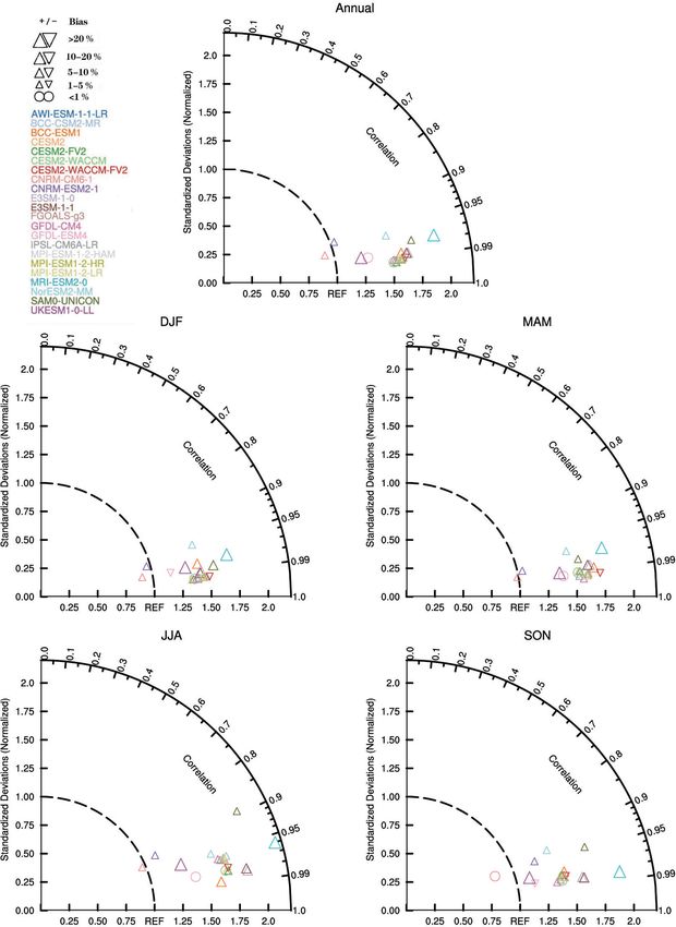
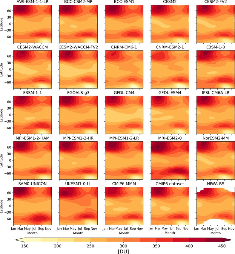
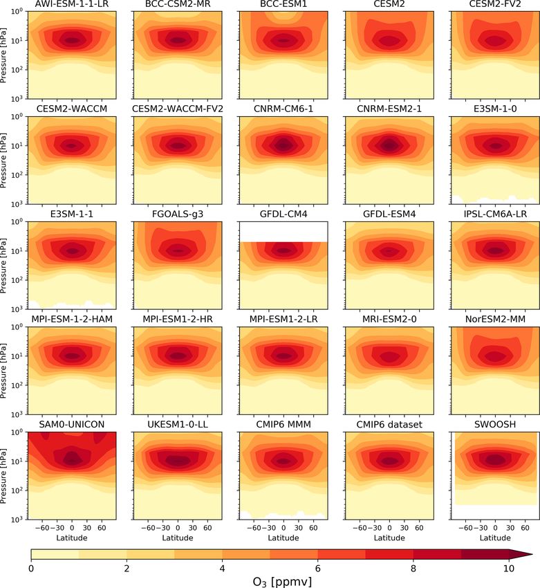
Figure 1. Latitude vs. altitude annual mean, zonal mean ozone mixing ratios (ppmv), averaged from 2000 to 2014, for each CMIP6 model, the
CMIP6 MMM, the CMIP6 ozone dataset used by models prescribing stratospheric ozone, and the SWOOSH combined dataset. GFDL-CM4
did not provide ozone output in the upper stratosphere, while the SWOOSH combined dataset only extends from ∼ 300 to 1 hPa.
3.1.1 The 2000–2014 climatological zonal mean and the quasi-equilibrated photochemical regime (e.g. Haigh and
total column ozone Pyle, 1982; Meul et al., 2014; Chiodo et al., 2018; Nowack
et al., 2018).
Notable differences between the models occur in the up-
Latitude–height cross sections of zonal mean ozone volume permost stratosphere and around the tropopause (Appendix
mixing ratios for each CMIP6 model, the CMIP6 MMM, Fig. A1). In the upper stratosphere, the BCC-ESM1, CESM2,
the CMIP6 ozone dataset used by models prescribing ozone CESM2-FV2, FGOALS-g3, NorESM2-MM, and SAM0-
mixing ratios, and the SWOOSH dataset, averaged over the UNICON models all simulate much higher ozone mixing ra-
years 2000–2014, are shown in Fig. 1. There is generally tios than the CMIP6 MMM (see Fig. A1). Additionally, the
good agreement between the individual CMIP6 models and BCC-ESM1 and SAM0-UNICON models also have a dif-
the SWOOSH dataset. All models broadly capture tropo- ferent spatial structure in the distribution of ozone at these
spheric and stratospheric ozone gradients, with a clear peak levels, with maxima in the midlatitudes at 1 hPa (see Fig. 1).
in ozone mixing ratios in the tropical stratosphere at around However, note that these models have lower model tops than
10 hPa, the downwards bending of the contour lines towards the 1 hPa maximum altitude of the CMIP6 data request, and
high latitudes in the lower stratosphere (e.g. Plumb, 2002)
and flat contour lines in the tropical upper stratosphere in
https://doi.org/10.5194/acp-21-5015-2021 Atmos. Chem. Phys., 21, 5015–5061, 20215026 J. Keeble et al.: Evaluating stratospheric ozone and water vapour changes
cal tropopause region. Both MRI-ESM2-0 and UKESM1-0-
LL are high biased, while BCC-ESM1 and SAM0-UNICON
are biased low compared to the observations and the CMIP6
MMM.
TCO climatologies (latitude vs. month), averaged over
the years 2000–2014, for the individual CMIP6 models, the
CMIP6 MMM, the CMIP6 ozone dataset, and the NIWA-
BS dataset are shown in Fig. 3. Overall, the observed clima-
tology patterns and annual cycle amplitudes, compared here
against the NIWA-BS dataset, are well represented in the
CMIP6 MMM and the individual models: lower values and
smallest amplitude in the tropics that increase to the poles,
with the highest TCO values around 60◦ S between August
and November, and in the NH polar regions between Jan-
uary and May, and the smallest TCO values in the SH po-
lar regions during the ozone hole period. However, despite
this good qualitative agreement between the CMIP6 models
and the NIWA-BS observational dataset, there is significant
variation between individual CMIP6 models with respect to
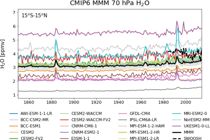
Figure 2. Climatological (2000–2014) seasonal cycle of ozone the CMIP6 MMM (Fig. A2). CNRM-CM6-1 and CNRM-
(in ppmv) at 70 hPa (15◦ S–15◦ N average) for CMIP6 models, the ESM2-1 underestimate TCO in the polar regions, while over-
CMIP6 MMM (solid black line), and SWOOSH combined ozone estimate TCO in the tropics, while the MRI-ESM2-0 and
dataset (dashed black line). The light grey envelope indicates the UKESM1-0-LL models overestimate TCO globally. Of par-
model spread about the MMM, calculated as the standard error of ticular note are the MRI-ESM2-0 and SAM0-UNICON mod-
the mean. els, which have large positive TCO anomalies with respect to
the CMIP6 MMM at high southern latitudes in the spring, in-
dicating they underestimate Antarctic polar ozone depletion.
so these differences arise from interpolation to the pressure Despite the differences between the individual CMIP6
levels of the CMIP6 data request. models, there is generally good agreement between the
In the tropical tropopause region, the MRI-ESM2-0 and zonal mean distribution of ozone in the CMIP6 MMM and
UKESM1-0-LL models significantly overestimate ozone the SWOOSH dataset throughout much of the stratosphere
mixing ratios, while the SAM0-UNICON model has much (Fig. 4), with differences between 70 and 3 hPa typically
lower mixing ratios in this region with respect to the less than ± 15 %. Maximum ozone mixing ratios at ∼ 10 hPa
CMIP6 MMM. The tropical tropopause is a region in which are slightly underestimated by the CMIP6 MMM, while
chemistry–climate models have typically performed poorly, ozone mixing ratios in the lower tropical stratosphere, and
due to the fact that ozone mixing ratios in this region are at ∼ 1 hPa in the midlatitudes, are overestimated (consistent
controlled by a combination of chemical production, vertical with the analysis shown in Fig. 2). The CMIP6 MMM also
transport of ozone poor air from the troposphere and mix- overestimates ozone mixing ratios at all latitudes in the upper
ing of ozone-rich stratospheric air. Gettelman et al. (2010) troposphere between 200–100 hPa by ∼ 20 %–40 %. Since
documented the seasonal cycle of ozone at 100 hPa from 18 upper tropospheric ozone is a particularly important climate
models involved in the CCMVal-2 intercomparison project forcing agent (Lacis et al., 1990; Stevenson et al., 2013;
and showed that while there is good agreement between Young et al., 2013; Nowack et al., 2015; Banerjee et al.,
the MMM and the observations, there is a large spread in 2018), this has important implications for the ozone radiative
ozone mixing ratios between individual models, and many forcing estimated from climate model simulations. However,
models do not accurately capture the observed seasonal cy- it should be noted that the uncertainties in the SWOOSH
cle. For the CMIP6 models investigated here, there is also dataset are likely to be relatively large in the upper tropo-
good agreement between the climatological (2000–2014), sphere.
tropical (15◦ S–15◦ N) MMM ozone mixing ratios at 70 hPa, The lower row of Fig. 4 shows the TCO differences be-
and the SWOOSH dataset (Fig. 2), both for the absolute tween the CMIP6 MMM and the NIWA-BS dataset. In the
ozone mixing ratios and the amplitude of the seasonal cy- tropics and the NH midlatitudes, the differences are smaller
cle. Many CMIP6 models accurately capture the seasonal cy- than ± 10 DU (< 5 % of the climatological value in these re-
cle of ozone, with lower ozone mixing ratios simulated be- gions). The differences get slightly larger in the NH polar re-
tween February and April, and higher values in August and gions but are largest in the SH midlatitudes and high latitudes
September. However, as with CCMVal-2 models, there is a where the MMM overestimates the observed TCO by up to
large spread in modelled ozone mixing ratios in the tropi- 25 DU throughout much of the year, except during late spring
Atmos. Chem. Phys., 21, 5015–5061, 2021 https://doi.org/10.5194/acp-21-5015-2021You can also read