The State of Climate Modeling in the Great Lakes Basin - A Synthesis in Support of a Workshop held on June 27, 2019 in Ann Arbor, MI
←
→
Page content transcription
If your browser does not render page correctly, please read the page content below
The State of Climate
Modeling in the Great
Lakes Basin
A Synthesis in Support of a Workshop
held on June 27, 2019 in Ann Arbor, MI

                                         Report By: Ontario Climate
                                         Consortium

                                         Date: September 13, 2019
Acknowledgements:
This synthesis report has been prepared in partnership by the Ontario Climate Consortium (OCC), and
Environment and Climate Change Canada. The authors wish to acknowledge the following individuals for
their contributions to this project:

Kristina Dokoska, Ontario Climate Consortium
Nishal Shah, Ontario Climate Consortium
Greg Mayne, Environment and Climate Change Canada
Wendy Leger, Environment and Climate Change Canada
Frank Seglenieks, Environment and Climate Change Canada
Armin Dehghan, Environment and Climate Change Canada
Shaffina Kassam, Environment and Climate Change Canada
Heather Arnold, Environment and Climate Change Canada
Shivani Vigneswaran, Environment and Climate Change Canada

Recommended Citation:
Delaney, F. and Milner, G. 2019. The State of Climate Modeling in the Great Lakes Basin - A Synthesis in
      Support of a Workshop held on June 27, 2019 in Ann Arbor, MI. Toronto, Canada.

                                                                      www.climateconnections.com |     2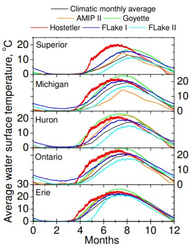
Table of Contents
Executive Summary .......................................................................................................................................................................... 4
1. Introduction ................................................................................................................................................................................... 7
      1.1 The Great Lakes Basin ........................................................................................................................................................ 7
      1.2 Climate Change Impacts and the Need for Climate Modeling in the Great Lakes Basin ..................................................... 7
      1.3 Objectives of this Report and Workshop .............................................................................................................................. 8
2. Background................................................................................................................................................................................... 8
      2.1 Global Circulation Models (GCMs) and Regional Climate Models (RCMs) ......................................................................... 8
      2.2 Downscaling Methods ........................................................................................................................................................ 10
      2.3 Ensemble Approach .......................................................................................................................................................... 11
      2.4 Climate Change Scenarios ................................................................................................................................................ 12
3. An Overview of Climate Models that Incorporate Great Lakes Conditions.................................................................................. 14
      3.1 Taking Stock of Models in the Great Lakes: An Inventory ................................................................................................. 14
        3.1.1 Global Circulation Models (GCMs) ................................................................................................................................ 14
        3.1.2. Regional Climate Models (RCMs) ................................................................................................................................ 16
        3.1.2.1.Ensembles Available for Use in the Great Lakes Basin ............................................................................................. 19
        3.1.3. Hydrodynamic Models .................................................................................................................................................. 29
      3.2 Limitations, Gaps and Uncertainties .................................................................................................................................. 32
4. Applying Climate Model Information across the Great Lakes Basin ........................................................................................... 35
      4.1 Users of Climate Model Information................................................................................................................................... 35
      4.2 Climate Service Providers across the Great Lakes Basin.................................................................................................. 37
      4.3 Common Approaches Applied in Great Lakes Basin ......................................................................................................... 38
5. Recommendations for Climate Modelers, Translators, and Users .............................................................................................. 41
6. Conclusions and Next Steps ....................................................................................................................................................... 45
7. References ................................................................................................................................................................................. 46
Appendix A: Stakeholder Workshop Agenda .................................................................................................................................. 58
Appendix B: Overview of Climate Change Modeling Experts Workshop, June 27, 2019 ................................................................ 60
Appendix C: Detailed Inventory of 1-Dimensional Climate Models in the Great Lakes ................................................................... 70
Appendix D: Detailed Inventory of 3-Dimensional Climate Models in the Great Lakes ................................................................... 72
Appendix E: List of 41 Studies Reviewed for Analysis of Climate Models Uses by Practitioners in the Great Lakes Basin ........... 73
Appendix F: Comparison of Projected Changes in the Great Lakes Basin for RCP8.5 - representative of Southwestern, ON,
Canada* .......................................................................................................................................................................................... 78

                                                                                                                                     www.climateconnections.com |                                  3
Executive Summary
The Great Lakes Basin (GLB) is one of the planet's largest freshwater ecosystems and is a vital source of
drinking water for over 20 million people. In recent decades, the GLB has felt the impacts of climate
change. These changes include higher temperatures, increased precipitation, reduced snow cover, abrupt
lake warming, decreased annual lake ice coverage, increased wind speeds and waves, fluctuating lake
levels, changes in timing and quantity of precipitation events, and an increased number of extreme
weather events (Wang et al., 2017). These changes are and will continue to have a significant impact on
the GLB’s natural assets and population including but not limited to increased flooding, erosion of
shorelines, contamination of water, and/or the loss and alterations of habitats for a variety of aquatic
species (Mortsch, 1998). It is thus important that sound scientific projections of these climatic changes
exist to assess the extent of the impacts of climate change within the GLB, and to communicate these
impacts with GLB communities and residents. This report provides a summary of the state of climate
modeling in the GLB and assesses model strengths and limitations, the knowledge gaps climate modelers
face, the state of climate model users and translators, and recommendations for modelers, users, and
translators moving forward.
The state of climate modeling in the Great Lakes has enhanced significantly in the past few decades.
Global Climate Models (GCMs) have traditionally been used to characterize the Earth's climate through
the modeling of the ocean-atmosphere circulation. The coarse spatial resolution that these models
operate on creates challenges for the GLB. Most climatological studies in the GLB now use Regional
Climate Models (RCMs) which offer higher resolution, dynamically downscaled GCM output under a more
regional climate context. This increased resolution allows for a more accurate representation of
climatological variables across hydrological features, which are typically represented as land surfaces on
GCMs.

Efforts have been made in creating one- and three-dimensional hydrodynamic models for specific
phenomena of the Great Lakes, and many modelers have started to couple these models with RCMs or
GCMs to better predict climate impacts across the GLB. While there have been significant strides in
climate change projections for the GLB, there exist numerous gaps in data collection, model
development, and in the general understanding of the Great Lakes and their interactions from outside
influences, such as large teleconnection patterns from the Gulf of Mexico and the Atlantic Ocean.

                                                                       www.climateconnections.com |      4
Current State of Knowledge Gaps in Data and Monitoring, Model Development, and of the Great
Lakes themselves:
The following provides a summary of the gaps identified in the literature review undertaken on climate
modeling for the Great Lakes:
1. Data and Monitoring Gaps
➢ Urban and agricultural land use
➢ Lake surface and profile temperatures
➢ Ice cover and ice thickness (e.g., areas of ridging and rafting)
➢ Energy exchanges and interfaces of land, lakes, ice, atmosphere, and hydrologic system
➢ Over-lake precipitation
➢ Over-lake evaporation
➢ Evapotranspiration
➢ Lake depth and opacity
➢ Eddy flux evaporation Lake circulation patterns
➢ Lake-effect snow (e.g., gridded products on snowfall and snow depth)
2. Gaps in Global, Regional, and Hydrodynamic Models in the Great Lakes Basin
➢ Teleconnections from large scale storms are not well captured over the Great Lakes because
atmospheric dynamics are poorly represented
➢ Groundwater, base flow, and rivers are not represented in models
➢ Snowbelt zones are often underestimated
➢ Ice cover can be overestimated in 1D lake models
➢ Seasonal stratification in lakes is not always well predicted, and the water temperatures near the
bottom of the Great Lakes are often misrepresented
➢ Thermal stratification beneath ice cover and radiative warming and mixing of near-surface water in
the spring is not well represented
➢ Turbulence models tend to over-predict mixing in smaller lakes
➢ Lake surface temperature (LST) boundary conditions are usually poorly estimated.
➢ Models lack the resolution required to incorporate realistic lake-effect morphology
➢ Most models lack the ability to model historical climate patterns over the Great Lakes
➢ Lack of seasonal predictions of climate; often models predict annual conditions
3. Knowledge Gaps in Understanding the Great Lakes in General
➢ Lack of understanding on the impacts of reduced ice cover and warmer LSTs on lake effect
precipitation
www.climateconnections.com | 5➢ Lack of understanding on temporal variations in the occurrences of harmful algal blooms and their
relationships to climate change
➢ Lack of understanding of the impacts of teleconnections (e.g., Polar vortex) and their impact on
the Great Lakes, and the lack of understanding on how teleconnection patterns will change with
climate change
➢ Lack of understanding on the water quality impacts on rivers and Great Lakes from storm
dynamics as well as nutrients and chemicals from urban and agricultural land use changes.
➢ Lack of understanding of the future of Great Lakes water levels and how these will change with
climate change.
➢ Lack of understanding the causes and effects of rapid warming the GLB has experienced in recent
years.
➢ Lack of understanding of lake-effect morphology on the Great Lakes and inter-lake differences in
warming trends and sensitivity.
Recommendations
From the knowledge gaps listed above, a set of recommendations have been provided for climate
modelers, information translators, and practitioners moving forward, these include:
1. Increase two-way coupling of models that incorporate the atmosphere, land, and lakes and
increase research and funds to 3D modeling.
2. Enhance data collection and conduct targeted field studies on lake climatology to feed into and
validate climate models, and enhance spatial-temporal data coverage.
3. Develop a shared set of data collection tools for operational users, climate modelers, and weather
forecasters to project socio-economic impacts to residents of the GLB.
4. Conduct continuous diverse stakeholder engagement between climate modelers, users,
translators, and funding agencies.
5. Continue to emphasize the connections between climate projections and local impacts.
6. Increase communication on the comparison of various climate model ensembles to practitioners.
7. Promote the importance of consistent approaches, where possible, being applied across similar
regions in the GLB.
8. Build emerging climate information into existing portals and tailor its output, where possible, for
different user groups.
9. Bolster available resources and opportunities to focus funding, specifically for Great Lakes scale
climate modeling initiatives.
www.climateconnections.com | 61. Introduction
1.1 The Great Lakes Basin
The five Laurentian Great Lakes are part of one of the world’s largest surface freshwater ecosystems,
spanning two Canadian provinces and eight states in the United States. Together, the Great Lakes
contain nearly 20% of the planet’s freshwater, providing drinking water to over 30 million people. The
Great Lakes Basin (GLB) provides opportunities for hydro generation, shipping, agriculture, fishing,
tourism, and recreation industries, and is part of the region’s physical and cultural heritage. However, the
impacts of industrialization, invasive species, toxic contaminants, agricultural runoff, and climate change
pose significant threats to the GLB’s well-being.
1.2 Climate Change Impacts and the Need for Climate Modeling in the Great Lakes
Basin
The Great Lakes play an important role in local weather patterns and climate processes due to their vast
sizes, depths, and degrees of thermal inertia. The Lakes produce many benefits to the GLB, as they
provide optimal environments for certain species to thrive due to the mild and cool breezes from the
Lakes. However, the Lakes also have the ability to cause infrastructure damage and disrupt critical
services from harsh lake-effect snow and ice storms (Sharma et al., 2018). The effects the Lakes have on
the climate have been studied for decades; however, there remain many knowledge gaps on the full
extent of services the Lakes provide to the region. In addition, as the climate continues to change
globally, the physical behaviour of the Great Lakes will also evolve over time, making it increasingly
difficult to project and predict future climates for the area. Limitations in climate modeling in the GLB can
inhibit our abilities to predict and communicate localized climate hazards and impacts, which increases
the vulnerability of people, ecosystems and infrastructure within the GLB.
In recent decades, the GLB has felt the impacts of climate change, generally consisting of higher
temperatures, increased precipitation, reduced snow cover, decreased annual lake ice coverage,
increased wind speeds and waves, fluctuating lake levels, changes in timing and quantity of precipitation
events, and an increased number of extreme weather events (e.g. snowstorms, ice storms,
thunderstorms, hailstorms, high wind speed events) (Wang et al. 2017). These changes in climate can
cause many cascading impacts, for example, variations in lake levels may lead to increased flooding
events, erosion of shorelines, contamination of water, and/or the loss and alterations of habitats for a
variety of aquatic species (Mortsch, 1998).
It is extremely important to plan for anticipated climatic changes and to reduce the negative impacts they
may cause. By enhancing the way we examine current conditions, projecting future climates in the GLB,
and communicating this information, decision-makers and resource managers will have the necessary
information to develop climate change adaptation policies to help residents of the GLB withstand the
negative impacts of climate change.
www.climateconnections.com | 71.3 Objectives of this Report and Workshop
Environment and Climate Change Canada (ECCC) initiated a collaborative workshop on climate modeling
in the Great Lakes Basin to be held in Ann Arbor, Michigan on June 27, 2019 to fulfill the objectives of
both Annex 7 (Habitats and Species) and Annex 9 (Climate Change Impacts) of the Great Lakes Water
Quality Agreement (GLWQA). Both annexes are working to bridge the gap between climate modelers and
decision makers, and to enhance collaboration and communication within the climate modeling
community.
Specifically, the objectives of the workshop and this report are to:
1. Review the existing Great Lakes regional climate modeling efforts, including the strengths,
limitations and credibility of climate change projections and their applicability to the Great Lakes
Basin;
2. Share preliminary results from relevant studies in Canada and the U.S.;
3. Identify gaps and areas of greatest uncertainty; and
4. Develop recommendations for future work.
By identifying the current gaps in climate modeling in the GLB, climate modelers and practitioners can
work together to improve these models through funding, collaboration, and engagement activities.
Appendix A provides an agenda of the day on June 27, 2019, and Appendix B provides an overview of
the entire workshop.
2. Background
To ensure all participants at the workshop had a foundational understanding of climate modeling, the
following section provides a brief background on climate modeling and key terminologies that will be used
throughout the rest of the report and during the workshop. This section discusses the differences between
Global Circulation Models and Regional Climate Models, various downscaling methods, ensemble
approaches, and the different climate change scenarios used in climate modeling.
2.1 Global Circulation Models (GCMs) and Regional Climate Models (RCMs)
Global Climate Models (GCMs) are coupled ocean-atmospheric models that project future changes in
climate over the entire Earth surface under alternative GHG emissions scenarios (Charron, 2016;
EBNFLO, 2010). These models develop climate projections with a horizontal resolution usually ranging
between 150 – 300 km, on continental scales (Wang et al., 2016) and are designed to characterize future
climate on an annual, seasonal and monthly basis (EBNFLO, 2010). In general, three different types of
GCMs exist: Atmospheric General Models (AGCMs), Atmospheric-Ocean General Circulation Models
(AOGCMs), and Earth System Models (ESMs) (Charron, 2016). AGMs were the first GCMs to be
developed. These models examine the atmospheric portion of the climate and its interaction with the land
www.climateconnections.com | 8surface. AOGCMs examine how the atmosphere and land interact with physical ocean models (Charron,
2016). Lastly, ESMs are the latest generation of models and include biogeochemical interactions and
cycles, as well as changes in land cover (e.g., vegetation types) (Charron, 2016). Since GCMs provide
projections over larger spatial scales, limitations exist. Some of the most prominent limitations to GCMs
are that GCMs cannot simulate smaller scale convective storms (i.e., thunderstorms), and as a result
cannot account for some extreme events at the local scale (EBNFLO, 2010). They also have deficient
land-atmosphere feedbacks; they lack the integration of lakes in the models; most are deficient in the
resolution of the planetary boundary layer (PBL) and do not include cloud processes; they have
insufficient surface heterogeneity; and they have dampened extreme weather conditions compared to
historical observations (Notaro, in person).
RCMs have emerged as an increasingly valuable climate model. RCMs are high resolution models that
are used to downscale the lower (or “coarser”) resolution GCM outputs, providing a physically realistic
simulation of climate projections over a smaller geographical area (ECCC, 2017; Charron, 2016). RCMs
produce climate projections on a much finer scale (ranging from 10 – 50 km, some even have resolutions
of 4km) and produce more regionally-relevant climate information (e.g., the effects of the Great Lakes)
than GCMs that can be evaluated against historical climate observations (Whan and Zwiers, 2015;
Charron, 2016). As a result, RCMs allow for a more precise representation of land features such as lakes
and rivers and ensures that consistency is maintained among different climate variables (Charron, 2016).
Unlike GCMs, RCMs can project smaller scale storms (e.g., finer resolution RCMs can project
thunderstorms), allowing the models to incorporate future storms and extreme events (EBNFLO, 2010).
As a physical model, RCMs also provide the benefit of linking the interaction of GHG emissions with other
components of the climate system (Charron, 2016). Given that RCMs are dynamically downscaled
models, ensuring a range of projections are used will be necessary to ensure GCM biases and errors are
not amplified.
www.climateconnections.com | 92.2 Downscaling Methods
Downscaling is the process of generating climate information from a GCM with coarse spatial resolution to
a finer spatial resolution (Wilby et al., 2004; Flint and Flint, 2012). The two types of approaches, statistical
downscaling and dynamical downscaling have been established to achieve detailed regional and local
atmospheric data (Castro et al., 2005).
Statistical downscaling is based on a statistical model that compares large-scale climate variables from
GCMs to smaller scale regional or local climate variables (Wilby et al., 2004). It relies on historical
relationships (also referred to as “stationary assumption”) among climate variables at different scales
(Auld et al., 2016). There are three types of statistically downscaled approaches that can be applied,
including weather classification schemes, regression models, and weather generators (Wilby et al., 2004).
As the impacts of climate change become more significant, using a stationary assumption (i.e. relying on
historical forcing conditions) will result in greater uncertainty among the statistically downscaled data, as
important feedback cycles in the climate are not accounted for in these projections (e.g., the impact of
warming temperatures and lake ice will exponentially increase the rate of lake effect snow and
evaporation). Thus, using a stationary assumption is not necessarily a recommended approach to be
taken to account for future changes in climate, particularly for extreme weather events, and processes
that are dependent on other climate forces. The approach taken in statistical downscaling is therefore not
physically verifiable (Wilby et al., 2004). Since statistical downscaling relies on historic relationships
among climate variables at various scales, using a statistical relationship based on present-day conditions
may not hold up under different forcing conditions in future climate projections, where the principle of
stationarity no longer applies (Wilby et al., 2004). In addition, it is commonly understood that most
statistical downscaling methods underestimate observed extremes, however, there are some statistical
techniques (e.g., the probability density function) that have been used (e.g., by the Wisconsin Initiative on
Climate Change Impacts – WICCI) that reproduce observed extremes and allows for probabilistic
assessments. Therefore, the type of statistical downscaling impacts the robustness of historical (and
future) climates.
Dynamical downscaling is based on a spatial-scale numerical atmospheric model, commonly referred to
as a RCM (Castro et al., 2005). Traditional dynamical downscaling incorporates GCM data to provide the
initial conditions, lateral boundary conditions, sea surface temperatures, and initial land surface conditions
(e.g., general topography, large bodies of water) (Xu and Yang, 2012). It then continuously integrates
RCMs using the initial data and the boundary conditions from the GCM to develop the projections (Xu and
Yang, 2012). Depending on the purpose of the dynamic downscaling, RCMs are able to develop four
types of downscaling including short-term weather simulations, seasonal predictions, regional weather
simulations, seasonal predictions, and climate prediction.
Both statistical and dynamical downscaling techniques rely on GCMs to drive local-scale modeling and
analysis, and ideally the uncertainty associated with GCMs should be transparent through the
downscaling process (Wilby et al., 2004). A summary of the key advantages and disadvantages of both
statistical and dynamical downscaling are provided in Table 1.
www.climateconnections.com | 10Table 1: Key advantages and disadvantages of downscaling techniques. (adapted from Hostetler et al.,
2011).
Statistical Dynamical
+ fast and inexpensive (relatively) + true simulation of high resolution forcing and
climate
+ high resolution (e.g., 4 km or less) + large, internally consistent set of atmospheric
and surface variable
+ multiple GCMs for ensembles and different + avoids stationary assumption (i.e. uses trends
emissions scenarios into the future that differ from the historical rates of
change, and incorporates feedback cycles)
- limited ability to account for finer scale - time consuming (e.g., requires debiasing)
topography (reducing ability to account for
features like orographic precipitation over
mountain ranges, or evaporation over lakes)
- may not conserve mass and heat - limited number of GCMs used
- uses stationary assumption (uses historical rates - added model biases
of change to model the future), and mostly only
models for precipitation and temperature
In addition, the Great Lakes Integrated Sciences and Assessments (GLISA) team at the University of
Michigan have been working to develop a downscaled climate data guide for the Great Lakes Region.
This short guidance document was initiated to aid practitioners in choosing or using downscaled data for
various different projects. For example, the guide explains the limitations of statistical downscaling for the
Great Lakes region, it recommends dynamical downscaling when an interactive lake model is included,
and it discusses spatial resolution misconceptions and techniques of how to downscale projections
further. For more information on this document, please contact GLISA.
2.3 Ensemble Approach
Previous research using AOGCMs to project future changes in climate has shown that no single model
exists that can determine all possible future climates (Tebaldi et al., 2004). Research has shown that the
use of a single model to project climate trends increases the number of errors within the climate modeling
and can result in a misinterpretation of climate trends (Auld et al., 2016). Each individual model
represents specific climatological processes and comes with its own set of biases (Sheffield et al., 2013).
The ensemble, or multi-model approach uses multiple models together to produce a full range of possible
climate scenarios and represents those projections using statistical distribution. Statistical distribution
allows the users to interpret trends probabilistically and address the uncertainties associated with the
climate modeling (Auld et al., 2016). Using a multi-model approach provides better predictions and
compares more favourably to observations than a single model (Auld et al., 2016). With the ensemble
www.climateconnections.com | 11approach, individual biases present in a single model tend to be reduced while the uncertainty associated
with the overall process is maintained and can be disseminated through further analysis and local-scale
modeling. Ensembles can consist of multiple GCMs coupled with a single or multiple RCMs, one GCM
coupled with multiple RCMs, or simply running one single model with an ensemble of “runs” (running the
model to multiple climate scenarios). An ensemble of RCMs requires that users first select the GCM(s)
that they wish to use followed by the selection of RCMs that they would like to downscale the GCM data
from (Evans et al., 2013). While there is no best future scenario that can be applied for any given
situation, the use of an ensemble approach allows for a more plausible approach to capture what the
future may represent (Charron, 2016).
GLISA has also created a Great Lakes Ensemble of future climate projections and guidance for
practitioners in the Great Lakes region, to increase the capacity of practitioners to be informed consumers
of climate information. Click here for more information on GLISA’s Great Lakes Ensemble.
2.4 Climate Change Scenarios
Another uncertainty associated with modeling and projecting climate is the future of human behaviour,
technology, and of the amount of carbon in the atmosphere. Therefore, in climate modeling, there exists a
series of plausible pathways, otherwise referred to as “scenarios”, or targets that embody the
relationships between human behaviour, emissions, greenhouse gas (GHG) concentrations, and
temperature change. The most recently produced climate change scenarios are called Representation
Concentration Pathways (RCPs), which have been endorsed by the Intergovernmental Panel on Climate
Change (IPCC). RCP scenarios consider the impacts of policies that may reduce GHG emissions
significantly (e.g., RCP 2.6), as well as the impact of the continued heavy reliance on fossil fuels (e.g.,
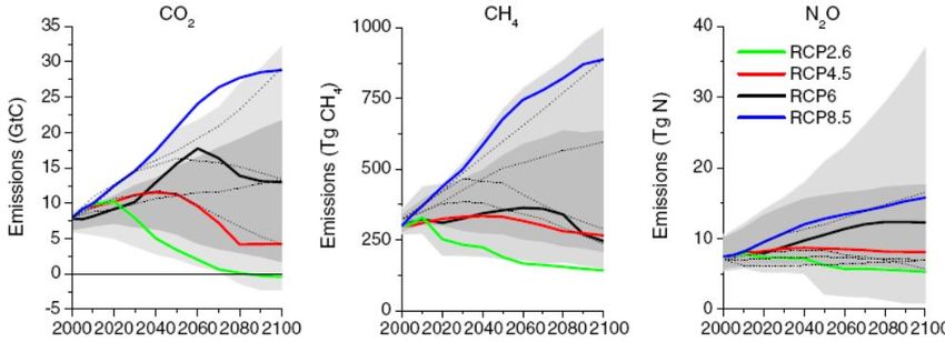
RCP 8.5). Figure 1 demonstrates the four RCP scenario projections through time, for three different
greenhouse gases.
Figure 1: Graphs demonstrating the four Representative Concentration Pathways (RCPs) for carbon dioxide (CO2)
methane (CH4), and nitrous dioxide (N2O) (Van Vuuren et al., 2011).
www.climateconnections.com | 12Prior to the development of the RCP climate scenarios, climate modelers across the globe used (and
some may still use) the SRES (Special Report on Emission Scenarios) climate scenarios, which do not
account for all of the different mitigative futures available in the RCP climate scenarios. One of the main
differences between the RCP and SRES climate scenarios is that RCP scenarios consider GHG
concentrations, while SRES scenarios consider GHG emissions; this is due to the fact that carbon
concentration in the atmosphere is not solely reliant on human-induced emissions, as the carbon cycle is
much more complex than this (e.g., the carbon emitted from trees, the amount of carbon absorbed by
oceans). Therefore, RCP climate scenarios are more commonly used, to account for the complexity of the
carbon cycle into the climate models and the SRES scenarios are not generally used in the latest climate
modeling exercises. Table 2 provides an overview of RCP concentration scenarios, with the comparative
SRES emissions scenarios for reference throughout this report.
Table 2: The four Representative Concentration Pathways that have been used in the Fifth Intergovernmental Panel
on Climate Change (IPCC) Assessment, with comparative SRES scenarios (IPCC, 2014).
SRES
Representative Temperature
Concentration Definition
Anomaly
Pathway (RCP)
Equivalent
The lowest emission scenario, where peak radiative forcing is 3
Wm-2 and declines before 2100 (IPCC, 2014). This scenario would
RCP 2.6 None require all the main GHG emitting countries, including developing
countries, to participate in climate change mitigation initiatives and
policies.
The second lowest emission scenario, where stabilization without
RCP 4.5 SRES B1 overshoot pathway to 4.5 Wm-2 and stabilization after 2100 (IPCC,
2014).
The second highest emission scenario, where stabilization without
RCP 6.0 SRES B2 overshoot pathway to 6 Wm-2 and stabilization after 2100 (IPCC,
2014).
The highest emission scenario, where rising radiative forcing
pathway leading to 8.5 Wm-2 in 2100, and continues to rise for some
RCP 8.5 SRES A1F1
amount of time (IPCC, 2014). GHG concentrations are up to
seven times higher than preindustrial levels.
In addition, GLISA is also developing a climate scenarios guide for practitioners, which frames SRES and
RCPs as one type of scenario in a larger chain of information used to create climate change and climate
impact scenarios (produced by climate impact assessment models and expert guidance). Please contact
GLISA for more information on their climate scenarios guidance document.
www.climateconnections.com | 133. An Overview of Climate Models that Incorporate Great Lakes
Conditions
3.1 Taking Stock of Models in the Great Lakes: An Inventory
One of the key drawbacks that practitioners and planners come across when developing adaptation
actions is the breadth of climate models that exist, and the complex language surrounding these. It is
often difficult to choose appropriate climate models or methods to predict the future climate for a given
area within the GLB. This section of the report will outline some of the GCMs, RCMs, and the more
complex hydrodynamic models that have been used in the GLB to date, followed by their limitations,
gaps, and uncertainties.
3.1.1 Global Circulation Models (GCMs)
Most GCMs were not designed with emphasis on lake-land-atmosphere interactions, despite the Great
Lakes’ influence on regional climate. As previously mentioned, GCMs usually have a horizontal resolution
that varies between 150 to 300 km, limiting the ability for GCMs to appropriately account for the Great
Lakes to a certain extent (e.g., the length of Lake Ontario is about 310 km). A study by GLISA (currently in
review) evaluates how all 55 GCMs within the Coupled Model Intercomparison Project Phase 5 (CMIP5)
models (models used in the latest IPCC report) incorporate the Great Lakes, if at all. The study showed
that 18 of the GCMs simulate all five of the Great Lakes as "dynamic lakes” (i.e. models that account for
certain lake-atmosphere feedbacks within the resolution of a GCM, in one-dimension), one simulates all
the Great Lakes as oceans, three GCMs treat the Great Lakes as a water surface, but do not treat them
as “dynamic” (i.e. do not account for lake temperature and lake ice cover feedbacks), four GCMs over
simplify the geography of the Great Lakes, and treat them as low-resolution oceans, four GCMs do not
have any form of lake representation, and nine had conflicts in the geographic representation of the Great
Lakes and were not clear on how fluxes between land, ocean, and atmosphere were integrated (see
Table 3 for more specific details). It should be noted that while this study shows which GCMs incorporate
the Great Lakes, there is still uncertainty around how effective some of these models model climate in the
area (e.g., some GCMs simulate all five Great Lakes as dynamic lakes, however, they may treat the lakes
as shallow lakes that freeze over completely in the winter).
www.climateconnections.com | 14Table 3: Summary of Great Lakes representation in each of the Global Circulation Models in the CMIP5
Ensemble (GLISA, in review).
www.climateconnections.com | 15It is important to consider the GCMs that incorporate the Great Lakes when developing a method for
climate modeling for a specific area in the GLB. GLISA therefore recommends using the GCMs that treat
all of the Great Lakes as dynamic lakes for climate analyses in the GLB. From these GCMs, RCMs can
be derived and the large grid cells can be downscaled to a more appropriate scale to evaluate climate at
the local level.
3.1.2. Regional Climate Models (RCMs)
RCMs are models derived and downscaled or reanalyzed from GCMs to a finer horizontal resolution,
usually varying from 10 to 50 km grids. This section provides an overview of the most common RCMs that
have been used in the GLB, and ensemble approaches that have been made available or used in
climatological studies.
Firstly, there are four RCMs that appear to be more commonly used in the GLB. These are:
1. Canadian Regional Climate Model 5 (CRCM5) (or an earlier version of the model)
2. Regional Climate Model 4 (RegCM4) (or an earlier version of the model)
3. Weather Research and Forecasting model (WRF)
4. Canadian Regional Climate Model 4 (CanRCM4) (or an earlier version of the model)
The following table (Table 4) delves into more detail on each of these RCMs, such as their spatial
resolutions, developers, and institutions they are hosted at. Please note that the spatial resolution of
these models may vary depending on the study; the table therefore notes different studies that the models
have been used in.
Table 4: Detailed descriptions of the most commonly used RCMs in the Great Lakes Basin.
Regional Studies where
Spatial Develo Institutio
Climate Description ensemble is used
Resolution per n
Model
CRCM5 The first CRCM was developed in 1991 50 km by 50 K. Universit Modeling in the Great
at the University of Quebec at Montreal km grids, Winger é du Lakes Basin:
(UQAM). This version of the RCM is centered on Québec Goyette et al., 2000
driven by the GCM Global the Great a
Environmental Multiscale model (GEM). Lakes, with a Montréal Martynov et al., 2012
This RCM is an example of a horizontal (UQAM)
collaborative effort between a modern resolution of
global operational forecast provider and 0.5° Model itself:
a university-based organization. Martynov et al., 2013
In 2002, Ouranos was created and its Scinocca and McFarlane,
Climate Simulations Team (CST) 2004
became responsible for the
development of the operational versions Šeparović et al., 2013
of the CRCM and to carry out the
www.climateconnections.com | 16climate-change projections. The S.
Ouranos CST got strongly involved in Biner OURAN
the development of later versions of the OS
model (CRCM4 and CRCM5)
RegCM4 The Regional Climate Model system 10 km by 10 Dickins Iowa Modeling in the Great
RegCM was originally developed at the km grid on et State Lakes:
National Center for Atmospheric al., National Bryan et al., 2015
Research (NCAR) in 1989 (Dickinson et 1989, Center
al., 1989, Giorgi and Bates, 1989). for Notaro et al., 2015
Since then it has undergone major Giorgi, Atmosph Bennington et al., 2014
updates in 1993 (RegCM2), 1999 1990 eric
(RegCM2.5), 2006 (RegCM3) and most Researc Hostetler et al., 1993
recently 2010 (RegCM4),and is now h
controlled by the International Centre (NCAR) Bates et al., 1995
for Theoretical Physics (ITCP).
The RegCM was the first RCM to be Martynov et al., 2010
documented in literature, and was the
first model used to create the first Holman et al., 2012
month-long, or “climate mode”
simulation (Giorgi 1990). Notaro et al., 2013
The model is a community model, and Model itself:
has been designed for use by a variety Giorgi et al., 2012
of scientists in both industrialized and
developing nations (Giorig et al., 2012). Elguindi et al., 2011
It is therefore public, open source, user-
friendly, and has a portable code that
can be applied to any region of the
world. The model can also be
interactively coupled to a 1D lake
model, a simplified aerosol scheme,
and a gas phase chemistry module.
Model improvements include the
development of a new microphysical
cloud scheme, coupling with a regional
ocean model, inclusion of full gas-phase
chemistry, upgrades of some physics
schemes (convection, planet boundary
layer (PBL), cloud microphysics) and
development of a non-hydrostatic
dynamical core.
www.climateconnections.com | 17WRF This is a mesoscale numerical weather Varying Skamar U Modeling in the Great
prediction system designed for both resolutions for ock et Arizona Lakes Basin:
atmospheric research and operational different al., National
forecasting applications. It features two applications 2008 Center Anderson et al., 2018
dynamical cores, a data assimilation (e.g., sea for
system, and a software architecture surface Atmosph d’Orgeville et al., 2014
supporting parallel computation and temperature eric
system extensibility. The model serves simulations Researc Gula and Peltier, 2012
a wide range of meteorological can have a h
applications across scales from tens of resolution of 5 (NCAR) Xiao et al., 2018
meters to thousands of kilometers. km by 1 km,
WRF can produce simulations based on eddy- Model itself:
actual atmospheric conditions (i.e., from simulations Skamarock et al., 2008
observations and analyses) or idealized can have a
conditions. WRF offers operational resolution of Powers et al., 2017
forecasting a flexible and 50 –100 m,
computationally-efficient platform, while fire Liang et al., 2012
reflecting recent advances in physics, simulations
numerics, and data assimilation can have a
contributed by developers from the resolution of
expansive research community. The 200 by 800 m)
model can provide a range of
predictions of phenomena such as air
chemistry, hydrology, wildland fires,
hurricanes, and regional climate. While
the WRF Model has a centralized
support effort, it has become a
community model, driven by the
developments and contributions of an
active worldwide user base.
www.climateconnections.com | 18CanRCM4 CanRCM4 was developed by employing 50 km by 25 Scinoc Canadia Modeling in the Great
a new approach of "coordinated" global km, or by ca et n Centre Lakes Basin:
and regional climate modeling. This 0.22° by 0.22° al., for Kerr et al., 2018
allows the model to incorporate or 0.44°by 2016 Climate
dynamical driving parameters (e.g., 0.44° Modeling
wind, temperature, moisture), and and Model itself:
allows for interpretation beyond the Analysis Scinocca et al., 2015
RCM’s lateral boundaries, as it is (CCCma)
coupled tightly with its GCM. CanRCM4 Scinocca et al., 2016
employs sea surface temperature and
sea ice distributions. The RCM is paired
with, and driven exclusively by, a global
parent model (GCM) for all of its
applications. CanRCM4's parent model
is CanAM4, which forms the
atmospheric component of the second
generation earth system model
CanESM2.
There are numerous RCMs that exist that offer detailed data on certain climate parameters; though it is
important to note that not all have detail on all parameters. Therefore, climate modelers have begun to
use ensembles of multiple RCMs or multiple RCM runs driven by different GCM boundary conditions, to
capture reduce bias in the projections they want to study, and to provide more robust and reliable
predictions (i.e. the more climate models that are used, the more likely the correct range of the future
climate will be predicted).
3.1.2.1 RCM Ensembles Available for use in the Great Lakes Basin
The following section delves into six ensembles of RCMs that are commonly used in the GLB
(NARCCAP, NA-CORDEX, Peltier Ensemble, Notaro Ensemble, USGS RCCV, University of Regina’s
Climate Portal, and York University’s LAMPS Climate Data Portal). The section discusses the strengths
and weaknesses of each of the RCM ensembles, and lists the various RCMs and GCMs used in each
one. This section aims to synthesize and summarize the state of the use of climate ensembles within the
GLB, to help practitioners choose a climate portal/ensemble in future climate modeling projects.
A) North American Regional Climate Change Assessment Program (NARCCAP) (this website
provides additional information)
www.climateconnections.com | 19The NARCCAP dataset contains high-resolution climate change scenario simulation outputs from multiple
RCMs derived from multiple Atmosphere-Ocean General Circulation Models (AOGCMs) for a 30-year
current and future periods. The RCMs are run at 50 km spatial resolution over a domain covering the
conterminous United States and most of Canada and results are recorded at 3-hourly intervals. The
driving AOGCMs are forced with the SRES A2 emissions scenario in the future period. This RCM
ensemble was created to examine the combined uncertainty in future climate projections from global to
regional models for North America.
NARCCAP uses five RCMs, which include:
• CRCM4 (Canadian Regional Climate Model Version 4)
• ECPC/ECP2 (Experimental Climate Prediction Center Regional Spectral Model)
• HRM3 (Hadley Regional Model Version 3)
• MM5I (Fifth Generation Pennsylvania State University – National Center for Atmospheric
Research (NCAR) Mesoscale Model)
• RCM34 (International Centre for Theoretical Physics – ITCP Regional Climate Model Version 3)
• WRFP/WRFG (Two versions of the Weather Research and Forecasting Model)
NARCCAP also uses four AOGCMs to drive each of the RCMs listed above. These include:
• CCSM3 (US National Centre for Atmospheric Research CCSM)
• MRI-CGCM3 (Meteorological Research Institute CGCM Version 3)
• GFDL CM2.1 (NOAA Geophysical Fluid Dynamics Laboratory Climate Model Version 2.1)
• HadCM3 (UK Met Office Hadley Centre Climate Model Version 3)
Strengths:
• One of the GCMs used in the ensemble simulates all five Great Lakes as dynamic lakes (e.g.,
MRI-CGCM3), while another treats part of the Great Lakes as oceans (e.g., HadCM3) (GLISA, in
review)
• Uses multiple RCMs and GCMs to strengthen overall results
•
• Consistent with historical observations in certain aspects (Wehner, 2012):
o Demonstrated that the western US had higher temperatures in coastal regions (except in
summer months) from 1971-2000, which is consistent with observations
o Demonstrated that temperatures were lower over mountainous regions and the Great
Plains, with a seasonal minimum in the winter, consistent with observations
Limitations:
• Some of the GCMs included in the ensemble do not show any form of representation of the Great
Lakes (e.g., GFDL CM2.1) (GLISA, in review), which may impact results
• There is great variation between the models (resolution, seasonality) (Wehner, 2012)
www.climateconnections.com | 20• Comparisons between observations and model outputs showed large east-west gradients, where
the eastern US had the greatest variation between the models
• Uses the previous version of CCSM (the latest model is CCSM2)
• Spatial resolution of 50 km square grid cells are too large to capture lake-effect patterns and for
decision makers interested in data at a local scale (e.g., across a watershed, municipality, region,
etc.)
• Uses the older climate change scenario of SRES A2
For more information on the evaluation of the NARCCAP climate ensemble with historical and future
predictions, see the following resources:
• Bukovsky, 2012: Temperature trends in the NARCCAP regional climate models
• Bukovsky et al., 2013: Towards assessing NARCCAP regional climate model credibility for
the North American Monsoon: Current climate simulations
• Horton et al., 2015: Projected changes in extreme temperature events based on the
NARCCAP model suite
• Karmalkar (2018): Interpreting results from the NARCCAP and NA-CORDEX ensembles
in the context of uncertainty in regional climate change projections
• Mearns et al., 2015: Uses of results of regional climate model experiments for impacts and
adaptation studies: The example of NARCCAP
• Mesinger et al., 2006: North American regional reanalysis
• Sobolowski and Pavelsky (2012): Evaluation of present and future North American
Regional Climate Change Assessment Program (NARCCAP) regional climate simulations
over the southeast United States
• Wehner, 2012: Very extreme seasonal precipitation in the NARCCAP ensemble: model
performance and projections
North American Coordinated Regional Climate Downscaling Experiment (NA-CORDEX) Ensemble
(refer to this website for more information):
This is an ensemble of six dynamically downscaled RCMs, which include:
• CRCM5 (Canadian Regional Climate Model 5)
• RCA4 (Rossby Centre Regional Atmospheric Model 4)
• RegCM4 (Regional Climate Model 4)
• WRF (Weather Research Forecasting model)
• CanRCM4 (Canadian Regional Climate Model 4)
• HIRHAM5 (Based on a subset of HIRLAM (High Resolution Limited Area Model) RCM and the
ECHAM ( European Centre developed at Hamburg) atmospheric general circulation model)
The RCMs listed above are run with six different GCMs, which include:
www.climateconnections.com | 21• HadGEM2-ES (U.K. Met Office Hadley Centre Earth System Model)
• CanESM2 (Second Generation Canadian Center for Climate Modeling and Analysis Earth System
Model)
• MPI-ESM-LR (Max Planck Institute for Meteorology Earth System Model LR)
• MPI-ESM-MR (Max Planck Institute for Meteorology Earth System Model MR)
• EC-EARTH (Irish Centre for High-End Computing EC-EARTH Model)
• GFDL-ESM2M (NOAA Geophysical Fluid Dynamics Laboratory Earth System Model Version 2M)
The ensemble is run for two different climate scenarios (RCP 4.5 and RCP 8.5) and the spatial resolution
varies from 12km to 25-km grids (depending on the different RCMs used and the different driving GCMs).
Strengths:
• Uses a wide range of GCMs to test and validate RCM projections across North America
• One of the GCMs treats all of the Great Lakes as dynamic lakes (e.g., GFDL-ESM2M), and
another treats the Lakes as a non-dynamic water surface (e.g., HadGEM2-ES) (GLISA, in review)
• All six RCMs are dynamically downscaled
• Freely accessible and accessible data portal
• Guidance documents on the use of the ensemble is provided on website
• Provides high resolution climate scenarios
Studies have shown the ensemble reproduces observed near-surface temperature and precipitation
over most of North America well, and represents the Great Plains Low-Level Jet stream well
(Martynov et al., 2013)
Limitations:
• Some of the GCMs included in the ensemble misrepresent the Great Lakes geographically in the
models (e.g., MPI-ESM-LR, CanESM2, EC-Earth) (GLISA, in review)
• Some climate variables are not yet available for download or are in development
• Practitioners may find downloading time longer given the size of the dataset available
• Studies have shown NA-CORDEX to misrepresent precipitation in the eastern half of the U.S. in
the winter, and the Great Plains in the summer (Karmalkar, 2018)
• Studies have shown the ensemble to show large variations in its ability to simulate observed
temperature trends (Karmalkar, 2018)
For more information on the evaluation of the NA-CORDEX climate ensemble with historical and future
predictions, see the following resources:
• Karmalkar (2018): Interpreting results from the NARCCAP and NA-CORDEX ensembles in the
context of uncertainty in regional climate change projection
www.climateconnections.com | 22• Diaconescu et al., (2017): Evaluation of CORDEX-Arctic daily precipitation and temperature-based
climate indices over Canadian Arctic land areas
• Giorgi et al. (2009): Addressing climate information needs at the regional level: the CORDEX
framework
• Lucas-Picher et al., (2013): Evaluation of the regional climate model ALADIN to simulate the
climate over North America in the CORDEX framework.
• Martynov et al., (2013): Reanalysis-driven climate simulation over CORDEX North America
domain using the Canadian Regional Climate Model, version 5: Model performance evaluation
Peltier Ensemble (refer to this report for more information):
This ensemble was initiated out of the University of Toronto. The ensemble is composed of physics-based
mini ensemble of five different physics configurations, using the U.S. Weather Research and Forecasting
(WRF) Model simulations dynamically downscaled from the National Center for Atmospheric Research
(NCAR) Community Earth System Model, version 1 (CESM1) GCM. The ensemble also uses the
freshwater lake model (FLake) (section 3.1.3 provides additional details on this model). The spatial
resolution of this ensemble is of 10-km grids, and all model runs are for the RCP 8.5 climate scenario.
Strengths:
• Incorporates the Great Lakes into models, using FLake
• Uses five physics components of the WRF to enhance climate projections
• Spatial resolution is very detailed at 10-km square grids
• Small biases in spatially-averaged temperature and precipitation (Peltier et al., 2017)
Limitations:
• Uses an outdated CCSM model (the latest version is CESM2)
• Uses one RCM and one GCM to drive climate projections
• Data is not available online as a standalone ensemble, but has been integrated into other portals
and other ensembles of models (e.g., York University’s LAMPS portal, which is described on page
17)
• Strong biases in areas of higher topography (Peltier et al., 2017)
• Does not include the influence of sulfate aerosol forcing (which can further exacerbate the cold
biases seen in the ensemble) (Peltier et al., 2017)
For more information on the evaluation of the Peltier climate ensemble with historical and future
predictions, see the following resources:
• Peltier et al., (2017): Uncertainty in Future Summer Precipitation in the Laurentian Great Lakes
Basin: Dynamical Downscaling and the Influence of Continental-Scale Processes on Regional
Climate Change
www.climateconnections.com | 23• Gula and Peltier (2012): Dynamical downscaling over the Great Lakes basin of North America
using the WRF regional climate model: The impact of the Great Lakes system on regional
greenhouse warming
• D’Orgeville et al., (2014): Climate change impacts on Great Lakes Basin precipitation extremes
• Erler et al., (2015): Dynamically downscaled high resolution hydroclimate projections for western
Canada
• Erler and Peltier (2016): Projected changes in precipitation extremes for western Canada based
upon high-resolution regional climate simulations
• Erler and Peltier (2017): Projected hydroclimate changes in two major river basins at the Canadian
west coast based upon high-resolution regional climate simulations
Notaro Ensemble (this website provides additional information):
This ensemble consists of one RCM, RegCM4, that downscales historical and future model output from
six different GCMs listed below:
• ACCESS1-0 (Australian Community Climate and Earth System Simulator)
• CNRM-CM5 (Centre National de Recherches Météorologiques)
• IPSL-CM5-MR (Institut Pierre Simon Laplace)
• MRI-CGCM3 (Meteorological Research Institute)
• MIROC5 (Model for Interdisciplinary Research on Climate Version Five)
• GFDL-ESM2M (National Oceanic and Atmospheric Administration Geophysical Fluid Dynamics
Laboratory)
The models chosen for the ensemble were based on statistical measures, resolution (e.g., the ratio
between parent and child models), bias magnitude in the Great Lakes region compared to observations
and climatology, range of future projections of regional temperature and precipitation, .
and representation of physical processes in the Great Lakes (e.g., hot/cold days, freeze-thaw cycles,
growing season length). The ensemble has been coupled with three one-dimensional models to
incorporate a lake, atmosphere, and land component (the Hostetler 1D lake model, the Pennsylvania
State University National Center for Atmospheric Research Mesoscale Model (MM5), and the Biosphere-
Atmosphere Transfer Scheme (BATS) – section 3.1.3 provides more information on these). The spatial
resolution of this ensemble is grids of 25-km and this ensemble provides data for 30 different climate
variables. All the models are run for the RCP 8.5 climate scenario, and all the GCMs that RegCM4 are ran
at incorporate the effects of the Great Lakes (GLISA, in review).
Strengths:
• Three GCMs used in this ensemble treat all Great Lakes as dynamic lakes (e.g., MRI-CGCM3,
MIROC5, GFDL-ESM2M), one that treats the Lakes as a non-dynamic water surface (e.g.,
ACCESS 1-0), and one that treats part of the Lakes as oceans (IPSL-CM5-MR) (GLISA, in review)
www.climateconnections.com | 24• 30 climate variables are available for download
• Freely accessible data and easy-to-use and interactive mapping website
• RegCM4 can reproduce the broad temporal and spatial patterns of lake ice and lake-effect
snowfall in the Great Lakes Basin (Notaro et al., 2013).
• RegCM4 accurately represents historical observed lake features (e.g., maximum and minimum
LSTs, ice cover, etc.) (Notaro et al., 2013).
• Thorough historical evaluations of the simulated climate and lake conditions were conducted and
compared to climate observations, giving the ensemble credibility.
Limitations:
• One GCM misrepresents the Great Lakes geographically (e.g., CNRM-CM5)
• Longer downloading time (e.g., each variable for each timeframe is about 670 NetCDF files in
total), however, access may can be granted to the server.
• RegCM4 is unable to simulate for remote climatic responses to the Great Lakes (e.g., beyond the
eastern U.S. and southeastern Canada), and the GCMs that do simulate these have inaccurate
representations of these phenomena due to their coarse grid sizes (Notaro et al., 2013).
• RegCM4 does not capture interannual variability in nlake ice and temperature (Bennington et al.,
2014).
For more information on the evaluation of the Notaro climate ensemble with historical and future
predictions, see the following resources:
• Bennington et al., (2014): Improving climate sensitivity of deep lakes within a Regional Climate
Model and its impact on simulated climate
• Holman et al. (2012): Improving historical precipitation estimates over the Lake Superior basin
• Notaro et al. (2013): Influence of the Laurentian Great Lakes on Regional Climate
USGS Regional Climate Change Viewer (RCCV) (refer to this report for more information):
The USGS has completed an array of high-resolution simulations of present and future climate over
Western and Eastern North America by dynamically downscaling four GCMs, using the RCM RegCM3,
and using PRISM (Parameter-elevation Relationships on Independent Slopes Model) data sets (which
calculates climate-elevation regressions for different elevations – gridded historical climate averages).
The four GCMs used in this ensemble include:
• NCEP (National Centers for Environmental Prediction)
• MPI ECHAM5 (Max Planck Institute for Meteorology (MPI) ECHAM5)
• GENMOM (combination of the GENESIS V3.0 and the MOM V2.0 oceanic GCM)
• GFDL CM 2.0 (NOAA Geophysical Fluid Dynamics Laboratory Climate Model Version 2)
www.climateconnections.com | 25You can also read