Interpreting Deep Learning Models in Natural Language Processing: A Review
←
→
Page content transcription
If your browser does not render page correctly, please read the page content below
Interpreting Deep Learning Models in Natural Language Processing:
                                                                            A Review

                                                                        Xiaofei Sun1 , Diyi Yang2 , Xiaoya Li1 , Tianwei Zhang3 ,
                                                                  Yuxian Meng1 , Han Qiu4 , Guoyin Wang5 , Eduard Hovy6 , Jiwei Li1,7
                                                                                 1
                                                                            Shannon.AI, 2 Georgia Institute of Technology
                                                                      3
                                                                        Nanyang Technological University, 4 Tsinghua University
arXiv:2110.10470v2 [cs.CL] 25 Oct 2021

                                                                5
                                                                  Amazon Alexa AI, 6 Carnegie Mellon University, 7 Zhejiang University

                                                                                                             Abstract
                                                     Neural network models have achieved state-of-the-art performances in a wide range of natural language processing (NLP)
                                                 tasks. However, a long-standing criticism against neural network models is the lack of interpretability, which not only reduces
                                                 the reliability of neural NLP systems but also limits the scope of their applications in areas where interpretability is essential
                                                 (e.g., health care applications). In response, the increasing interest in interpreting neural NLP models has spurred a diverse array
                                                 of interpretation methods over recent years. In this survey, we provide a comprehensive review of various interpretation methods
                                                 for neural models in NLP. We first stretch out a high-level taxonomy for interpretation methods in NLP, i.e., training-based
                                                 approaches, test-based approaches and hybrid approaches. Next, we describe sub-categories in each category in detail, e.g.,
                                                 influence-function based methods, KNN-based methods, attention-based models, saliency-based methods, perturbation-based
                                                 methods, etc. We point out deficiencies of current methods and suggest some avenues for future research. 1

                                         1       Introduction
                                         Deep learning based models have achieved state-of-the-art results on a variety of natural language processing (NLP) tasks
                                         such as tagging [127, 165, 217, 120], text classification [100, 221, 144, 121, 32, 199], machine translation [194, 59, 222, 187],
                                         natural language understanding [210, 110, 181, 200], dialog [4, 207, 16], and question answering [93, 97, 218, 208]. By
                                         first transforming each word (or each token in the general sense) into its word vector and then mapping these vectors into
                                         higher-level representations through layer-wise interactions such as recursive nets [175, 82, 117, 27], LSTMs [77], CNNs
                                         [95, 100], Transformers [194], deep neural networks are able to encode rich linguistic and semantic knowledge in the latent
                                         vector space [130, 41, 78, 71], capture contextual patterns and make accurate predictions on downstream tasks. However, a
                                         long-standing criticism against deep learning models is the lack of interpretability: in NLP, it is unclear how neural models deal
                                         with composition in language, such as implementing affirmation, negation, disambiguation and semantic combination from
                                         different constituents of the sentence [86, 203, 188]. The uninterpretability of deep neural NLP models limits their scope of
                                         applications which require strong controllability and interpretability.
                                         Designing methods to interpret neural networks has gained increasing attentions. in the field of computer vision, interpreting
                                         neural models involves identifying the part of the input that contributes most to the model predictions, and this paradigm has
                                         been widely studied (CV), using saliency maps [172, 211], layer-wise relevance propagation [13, 132, 102], model-agnostic
                                         interpreting methods [152] and back-propagation [171]. These methods have improved neural model interpretability and
                                         reliability from various perspectives, and raised the community’s awareness of the necessity of neural model interpretability
                                         when we want to build trustworthy and controllable systems [2, 191, 131]. Different from computer vision, the basic input units
                                         in NLP for neural models are discrete language tokens rather than continuous pixels in images [20, 38, 15]. This discrete nature
                                         of language poses a challenge for interpreting neural NLP models, making the interpreting methods in CV hard to be directly
                                         applied to NLP domain [22, 114]. To accommodate the discrete nature of texts, a great variety of works have rapidly emerged
                                         over the past a few years for neural model interpretability. A systematic review is thus needed to sort out and compare different
                                           1 E-mail addresses: xiaofei_sun@shannonai.com (X. Sun), diyi.yang@cc.gatech.edu (D. Yang), xiaoya_li@
                                         shannonai.com (X. Li), tianwei.zhang@ntu.edu.sg (T. Zhang), yuxian_meng@shannonai.com (Y. Meng), qiuhan@
                                         tsinghua.edu.cn (H. Qiu), guoyiwan@amazon.com (G. Wang), hovy@cmu.edu (E. Hovy), jiwei_li@shannonai.com (J.
                                         Li).

                                                                                                                  1
Training-based methods        Identify training instances responsible for the prediction of the current
                                           test instance.
             Test-based methods            Identify which part(s) of a test instance responsible for the model predic-
                                           tion.
             Hybrid methods                Identify because of which training instances, the model attends to which
                                           part(s) of the test instance for its prediction.

               Table 1: Summary of the high-level categories of interpretation methods for neural NLP models.

Figure 1: Difference of training-based, test-based and hybrid interpreting methods. The figure is adapted from the Figure 1 in
the work of [129]. In a nutshell, test-based methods target finding the most salient part(s) of the input; training-based methods
find the most contributive training examples responsible for a model’s predictions; hybrid methods combine both worlds, by
first finding the most salient part(s) of the input and then identifying the training instances responsible for the salient part(s).

methods, providing a comprehensive understanding of from which perspective a neural NLP model can be interpreted and how
the model can be interpreted effectively.
In this survey, we aim to to provide a comprehensive review of existing interpreting methods for neural NLP models. We
propose taxonomies to categorize existing interpretation methods from the perspective of (1) training-focused v.s. test-focused;
and (2) joint v.s. post-hoc. Regarding training-focused v.s. test-focused, the former denotes identifying the training instances or
elements within training instances responsible for the model’s prediction on a specific test example, while the latter denotes
finding the most salient part of the input test-example responsible for a prediction. The two perspectives can be jointly
considered: aiming to identify because of which training instances, the model attends to which part(s) of the test example for its
prediction. Based on the specific types of algorithms used, training-based methods can be further divided into influence-function
based methods, KNN-based methods, kernel-based methods, etc. Test-based methods can be divided into saliency-based
methods, perturbation-based methods, attention-based methods, etc. Figure 1 depicts the difference of training-based, test-based
and hybrid interpreting methods. Regarding joint v.s. post-hoc, for the former joint appraoch, a joint interpreting model is
trained along with the main classification model and the interpreting tool is nested within the main model, such as attention;
for the latter post-hoc approach, an additional probing model, which is separately developed after the main model completes
training, is used for interpretation. Figure 2 depicts the difference between joint and post-hoc approaches. Categorization with
taxonomy framework naturally separates different methods and makes audience easy to locate the works of interest. Table 1
shows the high-level categories of explanations
We analyze the literature with respect to these dimensions and review some of the representative techniques regarding each of
these categories. In summary, this work:
    • Categorizes interpreting methods according to training-focused v.s. test-focused and joint v.s. post-hoc.
    • Provides an empirical review of up-to-date methods for interpreting neural NLP models.
    • Discusses deficiencies of current methods and suggest avenues for future research.
The rest of this survey is organized as follows: Section 2 clarifies the high-level taxonomy proposed in this work. Section 3, 4
and 5 review existing training-based methods, test-based methods and hybrid methods for interpreting neural NLP models.
Section 6 discusses some open problems and directions that may be intriguing for future works. Section 7 summarizes this
survey.

                                                                 2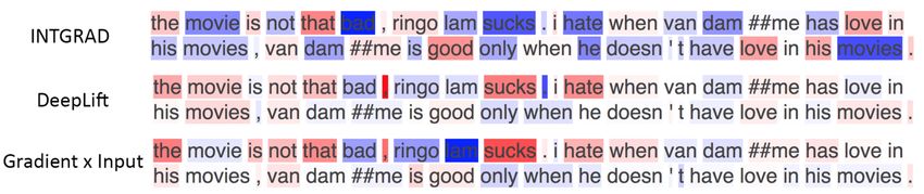
Figure 2: An illustrative comparison between joint interpreting methods and post-hoc interpreting methods.

1.1     Related Surveys
Related to this work, [216] conducted a survey of neural network interpretability methods used in computer vision, bioin-
formatics and NLP along several different dimensions such as using passive/active interpretation approaches or focusing
on local/global effect. However, our survey provides an in-depth overview for interpreting neural NLP models for NLP
tasks. Another line of work, AllenNLP Interpret [198], provides interpretation primitives (e.g., input gradients) for AllenNLP
model and task, a suite of built-in interpretation methods, and a library of front-end visualization components; the toolkit
mainly supports gradient-based saliency maps and adversarial attacks. In contrast, our review covers more comprehensive
interpretability methods.

2      High-level Taxonomy
In this section, we provide a high-level overview of the taxonomy used in this survey. As shown in Table 2, the topmost level
categorizes existing methods by whether they aim to interpret models from the training side, from the test side, or from both
sides.
Walking into the second level, this taxonomy categorizes literature based on the basic tools they use to interpret model behaviors.
For training-based methods, they are sub-categorized into influence functions (Section 3.1), KNNs for interpretation (Section
3.2) and kernel-based explanation (Section 3.3), which are respectively related to using influence functions, k nearest neighbors
and kernel-based models for interpretation in the training side. Test-based methods (Section 4) are sub-categorized into saliency
maps (Section 4.1), attention as explanation (Section 4.2.1), and explanation generation (Section 4.3), which respectively use
saliency maps, attention distributions and explainable contexts to interpret models in the test side. Hybrid methods interpret
model predictions by jointly examining training history and test stimuli, which can be viewed as a combination of training-based
and test-based methods (Section 5). Each category is paired with whether they belong to joint or post-hoc. In the following
section of this survey, we will expound on some of the representative works from each of the categories.

3      Training-Based Interpretation
The main purpose of training-based methods is to identify which training instances or units of training instances in the training
set are responsible for the model’s prediction at a specific test example. Existing training-based techniques fall into the following
three categories:
      • Influence function based interpretation: using influence functions to estimate the influence of each training point on
        an input test example. The training points with the highest influences are viewed as the most contributive instances.
      • Nearest Neighbor based interpretation: extracting the k nearest neighbor points in the training set that are close to an
        input test example. Extracted nearest neighbors are viewed as the most contributive instances
      • Landmark based interpretation: An input test sentence is fed to the classifier along with landmarks, which refer to
        a set of training examples used to compile the representation of any unseen test instance. The influence of training
        examples on an input test example is measured by the contribution of each landmark to the model’s decision on the

                                                                 3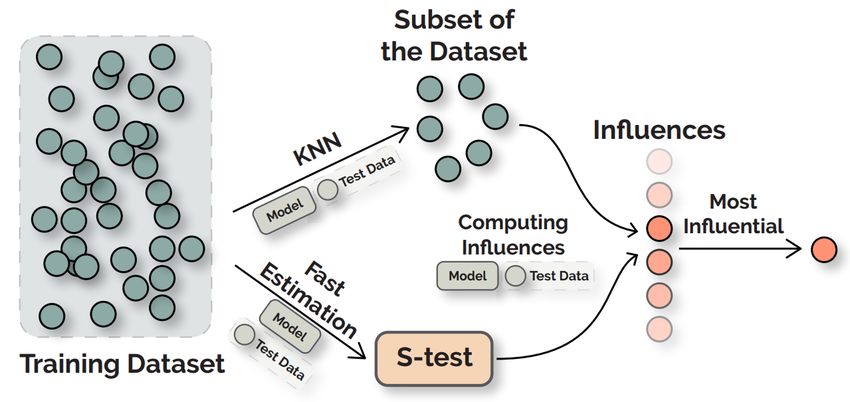
First Level       Second Level                Technique Description                                Joint/Post-   Representative Works
                                                                                                    hoc
                   Influence functions         Measuring the change in model parameters when        Post-hoc      [70, 103, 209, 69]
                                               a training point changes.
                   KNNs for interpretation     Searching k nearest neighbors over a model’s         Post-hoc      [197, 148]
 Training-based                                hidden representations to identify training exam-
                                               ples closest to a given evaluation example.
                   Kernel-based explanation    Within the kernel-based framework, selecting         Joint/Post-   [47, 48]
                                               landmarks that the Layer-wise Relevance Prop-        hoc
                                               agation algorithm highlights as the most active
                                               elements responsible for the model prediction.
                   Saliency maps               Computing the saliency score of each token or        Post-hoc      [116, 118, 184, 156, 6,
                                               span based on network gradient or feature attri-                   140, 61, 68, 99, 35]
                                               bution. The part of sentence with the highest
                                               salience score is viewed as the interpretable con-
                                               tent.
                   Attention as explanation    Leveraging attention distributions over tokens as    Joint         [182, 86, 164, 203, 193,
 Test-based                                    a tool of interpretation. The most attentive token                 154, 63, 41, 195, 190,
                                               or span is regarded as the most contributive to                    78, 30, 143, 71, 150]
                                               the model prediction.
                   Explanation generation      Generating or inducing explanations for the          Joint         [113, 134, 33, 185, 53,
                                               model’s prediction. The explanation may come                       87, 107, 149, 124, 56,
                                               from a subset of the input sentence, from exter-                   40, 79, 19, 161, 50, 153,
                                               nal knowledge or from a language model that                        147]
                                               generates explanations from scratch.
 Hybrid                                        Interpreting model behaviors by jointly examin-      Post-hoc      [129]
                                               ing training history and test stimuli.

Table 2: An overview of high-level taxonomy for interpretation methods in NLP. Column 1 denotes the topmost level of the
taxonomy. Column 2 denotes the second-level categorizations. Column 3 gives brief descriptions of the techniques grouped in
the second-level categorizations. Column 4 notifies whether the body of work is joint (the interpreting model is trained jointly
with the main model) or post-hoc (the interpreting method is applied to the trained main model). Column 5 contains a list of
representative references.

        test example based on the Layer-wise Relevance Propagation (LRP) [14] algorithm. As landmarks are organized via
        kernel-based deep architectures, this method is also referred to as Kernel-based Explanation.
We will describe these methods at length in the rest of this subsection.

3.1     Influence Functions Based Interpretation
3.1.1    Influence functions
The influence of a training point can be defined as the change in the model parameters when a specific training point is removed.
To measure the change of model parameters, an intuitive way is to retrain the model on the training set with the training example
left-out. However, this is prohibitively time-intensive as we need to retrain the model from scratch for every training example.
Alternatively, influence functions [45, 44, 104] provide an approximate but tractable way to track parameter change without the
need to repeatedly retrain the model.
Concisely speaking, the influence function estimates the impact on the model parameters when the loss of a particular training
point is up-weighted by a small perturbation . This can be done through first-order approximation. Let zi (i = 1, 2, · · · , n) be
a training point in the training set. The model parameters θ is learned to minimize a given loss function L:
                                                                       n
                                                                   1X
                                                   θ̂ = arg min          L(zi ; θ)                                                     (1)
                                                               θ   n i=1

Analogously, the optimal model parameters θz, when the loss of a training point z is weighted by a small perturbation can be

                                                                   4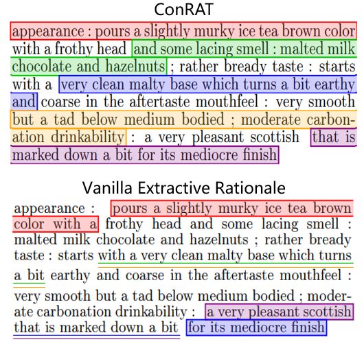
Figure 3: Efficient implementations of influence functions proposed in [103] (left) and [69] (right). The figures are borrowed
from the original literature.
derived by minimizing the following loss:
n
1X
θ̂z, = arg min L(zi ; θ) + L(z; θ) (2)
θ n i=1
By referring the audience to [104] for detailed proofs, the influence of a training point z on the model parameters θ, which is
denoted by I(z, θ), is given as follows:
dθ̂z,
I(z, θ) , = −Hθ−1 ∇θ L(z; θ̂) (3)
d
where Hθ , n1 zi ∇2θ L(zi ; θ̂) is the Hessian matrix over all training instances zi in the training set, and L(zi ; θ̂) is the loss of
P
z over model parameters θ. Equation 3 expresses the degree to which a small perturbation on a training point z influences the
model parameters θ. Based on Equation 3, [70] applied the chain rule to measure how this change in model parameters would
in turn affect the loss of the test input x:
dL(x; θ̂) dθ̂z,
I(z, x) , = ∇θ L(x; θ̂) · = ∇θ L(x; θ̂) · I(z, θ) = −∇θ L(x; θ̂)> Hθ−1 ∇θ L(z; θ̂) (4)
dz d
[70] defined the negative score −I(z, x) as the influence score. Equation 4 reveals that a positive influence score for a training
point z with respect to the input example x means that the removal of z from the training set would be expected to cause a drop
in the model’s confidence when making the prediction on x. By contrast, a negative influence score means that the removal of z
from the training set would be expected to give an increase in the model’s confidence when making this prediction. Experiments
and analysis from [70] validated the reliability of influence functions when applied to deep transformer-based [194] models.
3.1.2 Efficient influence functions
A closer look at Equation 4 reviews the disadvantage of influence functions: the computational cost of computing the inverse-
Hessian matrix Hθ−1 and iterating over all training points z to find the most (least) influential example is infeasible to bear
for large-scale models such as BERT [52]. Efficient estimates for influence functions are thus needed to improve runtime
efficiency while preserving the interpretability. [103] and [69] respectively address this issue from the model side and from
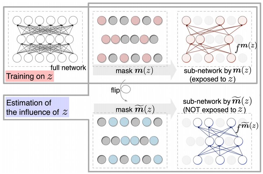
the algorithm side. Figure 3 illustrates how these two methods work. [103] proposed turn-over dropout, a variant of dropout
applied to the network for each individual training instance. After training the model on the entire training dataset, turn-over
dropout generates an individual-specific dropout mask scheme m(z) for each training point z, and then feeds z into the model
for training using the proposed mask scheme m(z). The mask scheme m(z) corresponds to a sub-network f m(z) , which is
updated when the model is trained on z, but the counter-part of the model f m̃(z) , is not at all affected. Therefore, the two
sub-networks, f m(z) and f m̃(z) , can be analogously perceived as two different networks trained on a dataset with or without z.
The influence of z on a test input example x can thus be computed as follows:
I(z, x) , L(x; f m(z) ) − L(x; f m̃(z) ) (5)
5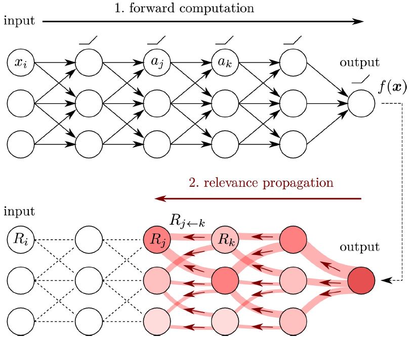
Figure 4: Overview of KNN-based (left, the figure is borrowed from the work of [148]) and kernel-based (right, the figure is
borrowed from the work of [48]) interpretation methods. KNN-based methods first cache high-dimensional representation of
training instances and search for the k nearest neighbors with respect to the test example in the latent space. Kernel-based
methods leverage landmark instances from the training set as part of the model input, providing linguistic evidence for
interpretation.

Experimenting on the Stanford Sentiment TreeBank (SST-2) [176] and the Yahoo Answers dataset [214] with the BERT model,
the turn-over dropout technique is able to interpret erroneously classified test examples by identifying the most influential
training instances, with a more efficient computation process. [69] tackled the computation issue of the original influence
functions from the algorithm perspective. Their optimization process can be divided into three aspects: (1) kNN constraint
on the search space; (2) the inverse Hessian computation speedup; and (3) parallelization. First, to avoid the global search
on the entire training dataset for the most influential data point, the search space is constrained within a small subset of the
training set. This can be achieved by selecting the top-k nearest neighbors to the test input instance x based on the l2 distance
between extracted features. Second, to speed up computation of the inverse Hessian matrix Hθ−1 , [69] carefully selected the
required hyperparameters used to compute the inverse Hessian matrix so that the inverse Hessian-vector product Hθ−1 ∇θ L(x; θ̂)
(Equation 4) can efficiently calculated. Third, [69] applied off-the-shelf multi-GPU parallelization tools to compute influence
scores in a parallel manner. The confluence of all three factors leads to a speedup rate of 80x while being highly correlated with
the original influence functions. With the new fast version of influence functions, a few applications that are concerned with
model interpretation but were previously intractable are demonstrated, including examining the “explainability” of influential
data-points, visualizing data influence-interactions, correcting model predictions using original training data, and correcting
model predictions using data from a new dataset. The efficient implementation of influence functions provide possibility for
new interpretable explorations that scale with the data size and model size.
The influence function based interpreting methods are along the post-hoc line, which means that they are applied for interpreta-
tion after the main model is fully trained.

3.2    KNNs Based Interpretation
KNN-based interpretation [197, 148] retrieves k nearest training instances that are the closest to a specific test input from
the training set. After the training process completes, each training point is passed to the trained model to derive its high-
dimensional representation z, which is cached for test-time retrieval. Then at test time, the model outputs the representation of
the input example x, uses it as the query to search for k nearest training instances in the cache store. In the meantime, the
distance between the query and each retrieved training point can be calculated, and the corresponding ground-truth labels for
the retrieved training points can also be extracted. The normalized distances are treated as the weight associated with each
training point the model retrieves to interpret its prediction for the test input example, and the percentage of nearest neighbors
belonging to the predicted class, which is called the conformity score [197], can be interpreted as how much the training data
supports a classification decision. [148] uses the conformity score to calibrate an uncertain model prediction, showing that KNN
interpretation is able to identify mislabeled examples. Figure 4 (left) provides an overview of the KNN-based interpretation
method proposed in [148].
KNN based interpretation works after the training process completes, and thus belongs to the post-hoc category.

                                                                6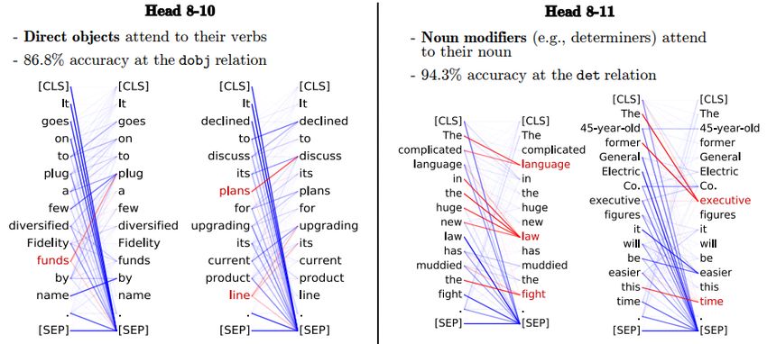
Figure 5: An overview of test-based methods. Left: The saliency score is the importance or relevance of a token or a span with
respect to the model prediction. A higher saliency score denotes greater importance. Middle: Attention scores over input tokens
reflects how the model distributes its attention to different parts of the input. Attention distributions can thus be viewed as a
tool for interpretation. Right: Given the input, the model gives its prediction as well as the evidence supporting its decision. A
judicious decision can be explained in a way of generating the corresponding explanations.

3.3    Landmark Based Interpretation
Landmark based interpreting methods [47, 48] use landmarks, which are a set of real reference training examples, to compile
the linguistic properties of an unseen test example. This line of methods combine the Layerwise Relevance Propagation (LRP)
[13] and Kernel-based Deep Architectures (KDAs) [46] to complete interpretation. An illustration is shown in Figure 4 (right).
More formally, given an input example x and d landmarks {l1 , l2 , · · · , ld } sampled from the training set, the model first
computes the similarity score K(x, li ) between x and each landmark li using a kernel function K(·, ·). Then, a Nyström layer
[204] is used to map the vector of similarity scores [K(x, l1 ), K(x, l2 ), . . . , K(x, ld )] to a high-dimensional representation.
Passing through multiple ordinary hidden layers, the model last makes its prediction at the classification layer. The expected
explanation is obtained from the network output by applying LRP to revert the propagation process, therefore linking the output
back to the similarity vector. Once LRP assigns a score to each of these landmarks (i.e., the corresponding similarity score
K(x, li )), we can select the positively active landmarks as evidence in favor of a class C. A template-based natural language
explanation is generated based on the activated landmarks. As an example given in [48], the generated explanation to the
input example “What is the capital of Zimbabwe?” that refers to Location is “since it recalls me of ‘What is the capital of
California?’, which also refers to Location”. In this example, “What is the capital of California?” is the activated landmark
used to trigger the template-based explanation, and Location is the class C the model predicts.
To decide whether the landmark–based model belonging to the joint or post-hoc category, we need to take into consideration its
two constituent components: (1) the kernel architecture component which involves the kernel function K(·, ·) and the Nyström
layer, and (2) the LRP scoring mechanism. For the former, the kernel architecture is trained together with the entire model and
therefore the landmark–based model can be viewed as along the joint interpretation line. For the latter, when computing the
importance of each landmark, LRP is a typical post-hoc interpreting method. The landmark–based model can thus be viewed as
both joint and post-hoc.

4     Test-Based Interpretation
Different from training-based methods that focus on interpreting neural NLP models by identifying the training points
responsible for the model’s prediction on a specific test input, the test-based methods, instead, aim at providing explanations
about which part(s) of the test example contribute most to the model prediction. This line of methods are rooted in the
intuition that not every token or span within the input sentence contributes equally to the prediction decision, and thus the most
contributive token or span can usually interpret the model behaviors. For example in Figure 1, the input test example “the movie
is fascinating” has a very typical adjective “fascinating” that would nudge the model to predict the class label Positive.
In this sense, the most contributive part is word “fascinating”. If we insert the negation “not” before “fascinating”, the most
contributive part would therefore be “not fascinating”, a span rather than a word in the input sentence.
Most of existing test-based methods fall into the following three categories: saliency maps, attention as explanation and
explanation generation. Saliency maps and attention provide very straightforward explanations in the form of visualized
heatmaps distributed to the input text, showing intuitive understandings of which part(s) of the input the model focuses most
on, and which part(s) of the input the model pays less attention to. The methods of textual explanation generation justify the
model prediction by generating causal evidence either from a part of the input sentence, from external knowledge resources or

                                                                 7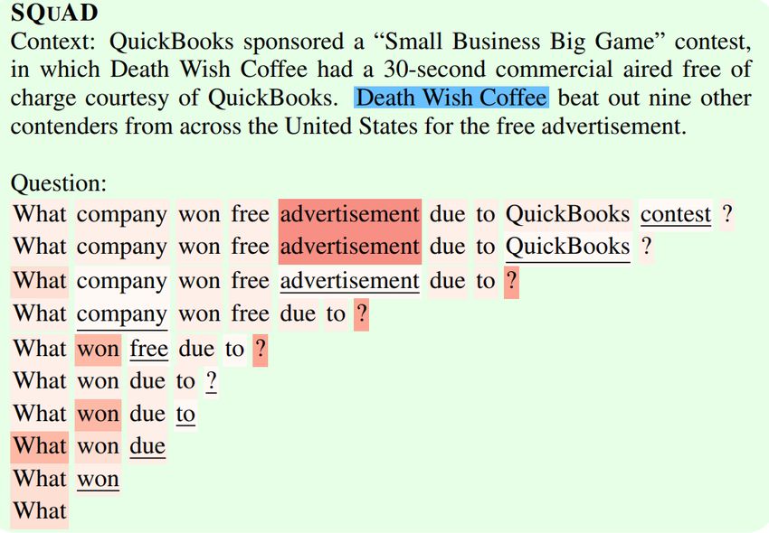
Method                                              Formulation
                                                                                       y       ∂S (x)
                       Vanilla Gradient                                 Score(xi ) = ∂x
                                                                                R 1 ∂Sy i(x̃)
                     Integrated Gradient              Score(xi ) = (xi − x̄i ) · α=0 ∂ x̃i x̃=x̄+α(x−x̄) dα
                         Perturbation                           Score(xi ) = Sy (x) − Sy (x\{xi })
                                                              (0)  (l)    P                   zji P                 (l+1)
                             LRP                Score(xi ) = ri , ri = j P 0 (z 0 +bj )+·sign(                    rj
                                                                                 i  ji             i0 (zji0 +bj ))
                                                                      (0)  (l)     P       z −z̄          (l+1)
                          DeepLIFT                     Score(xi ) = ri , ri = j P 0 z ji0 −Pji 0 z̄ 0 rj
                                                                                                 i   ji     i    ji

Table 3: Mathematical formulation of different saliency methods. LRP and DeepLIFT perform in a top-down recursive manner.

completely from scratch. This test-based framework of model interpretation, in contrast to training-based methods, is concerned
with one particular input example, and conveys useful and intuitive information to end-users even without any AI background.
Figure 5 shows a high-level overview for the three different strands of test-based methods. In the rest of this subsection, we will
describe each line of methods in detail.

4.1     Saliency-based Interpretation
In natural languages, some words are more important than other words in indicating the direction to which the model predicts.
In sentiment classification for example, the words associated with strong emotions such as “fantastic”, “scary” and “exciting”
would provide interpretable cues for the model prediction. If we could measure the importance of a word, or a span, and
examine the relationship of the most important part(s) with the model prediction, we will be able to interpret the model
behaviors through the lens of these important contents and their relationship with model predictions. The importance of each
token (or its corresponding input feature), which sometimes is also called the saliency or the attribution, defines the relevance
of that token with the model prediction. By visualizing the saliency maps, i.e., plotting the saliency scores in the form of
heatmaps, users can easily understand why model make decisions by examining the most salient part(s).
We describe four typical ways of computing the saliency score in the rest of this subsection. These methods include: gradient-
based, perturbation-based, LRP-based and DeepLIFT-based. Table 3 summarizes the mathematical formulations of these
methods.

4.1.1       Gradient-based saliency scores
Gradient-based saliency methods compute the importance of a specific input feature (e.g., vector dimension, word or span)
based on the first-order derivative with respect to that feature. Suppose that Sy (xi ) is output with respect to class label
y before applying the softmax function, and xi is the input feature, which is the ith dimension of the word embedding
x = {x1 , x2 , ..., xi , ..., xN } for word w in NLP tasks. We have:

                                                                                     ∂Sy (xi )
                                                  Sy (xi + ∆xi ) ≈ Sy (xi ) +                  ∆xi                                               (6)
                                                                                       ∂x
∂Sy (xi )                                                                                            ∂Sy (xi )
  ∂xi       can be viewed as the change of Sy (xi ) with respect to the change of xi . If              ∂xi       approaches 0, it means that Sy (xi )
                                                ∂Sy (xi )
is not at all sensitive to the change of xi .     ∂x        can thus be straightforwardly viewed as the importance of the word dimension
xi [116]:
                                                                              ∂Sy (x)
                                                               Score(xi ) =                                                                      (7)
                                                                               ∂xi
Equation 7 computes the importance of a single dimension for the word vector. To measure the importance of a word Score(w),
we can use the norm as follows:                           v
                                                          uX ∂Sy (xi ) 2
                                                          u
                                              Score(w) = t                                                              (8)
                                                               i
                                                                     ∂xi

or multiply the important vector with the input feature vector [51, 6]:

                                                                         X         ∂Sy (xi )
                                                            Score(w) =        xi                                                                 (9)
                                                                          i
                                                                                     ∂xi

                                                                         8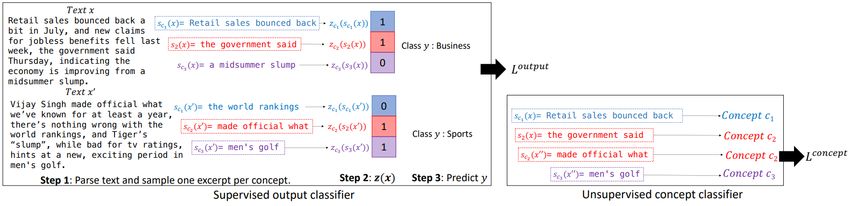
Figure 6: Diagram of the perturbation based method (left, the figure is brought from [61]) and LRP (right, the figure is brought
from [64]). Left: At each step, the least important word is removed by the saliency score using the leave-one-out technique. As
shown in the figure, the heatmaps generated with leave-one-out shift drastically: the word “advertisement” is the most salient in
step one and two, but becomes the least salient in step three. Right: LRP provides decomposition of the attribute scores from
the model prediction to the input features. It does not utilize partial derivatives but rather directly decomposes the activation
function to produce the attribute score.

Both methods work well for the interpretation purpose. Albeit simple and easy to implement, this kind of vanilla gradient
saliency score assumes a linear approximation of the relationship between the input feature and the model output, which is not
the case for deep neural networks. [184] proposed the integrated gradient (IG), a modification to the vanilla gradient saliency
score. IG computes the average gradient along the linear path of varying the input from a baseline value x̄ to itself x, which
produces a more reliable and stable result compared to the vanilla gradient approach. The baseline value is often set to zero. IG
can be formulated as the following equation:
                                                                 Z   1
                                                                         ∂Sy (x̃)
                                    Score(xi ) = (xi − x̄i ) ·                      x̃=x̄+α(x−x̄)
                                                                                                    dα                      (10)
                                                                 α=0      ∂ x̃i

4.1.2   Perturbation-based saliency scores
Perturbation-based methods compute the saliency score of an input feature by removing, masking or altering that feature,
passing the altered input again into the model and measuring the output change. This technique is straightforward to understand:
if a particular input token is important, then removing it will be more likely to causing drastic prediction change and flip the
model prediction.
One simple way to perturb an input is to erase a word from the input, and examine the change in the model’s prediction on the
target class label [118]. This technique is called the leave-one-out perturbation method. By iterating over all words, we can
find the most salient word that leads to the largest prediction change. The saliency score using leave-one-out can be given as
follows:
                                               Score(xi ) = Sy (x) − Sy (x\{xi })                                         (11)
The token-level removal can be extended to the span level or the phrase level [155, 206]. Based on the leave-one-out technique,
[61] uses input reduction, which iteratively removes the least salient word at a time, to induce the pathological behaviors of
neural NLP models. An example is shown in Figure 6 (left).
Another way to perturb the input is to inject learnable interpretable adversaries into an input feature [160, 68]. By conforming
to specific restrictions (e.g., the direction, the magnitude or the distribution) and learning to optimize predefined training
objectives, the adversarial perturbations are able to reveal some interpretable patterns within neural NLP models, such as the
word relationships, the information of each word discarded when words pass through layers, and how the model evolves during
training.

                                                                     9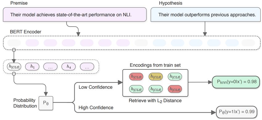
Figure 7: A visualization of saliency methods Integrated Gradient, DeepLIFT and Gradient×Input (the figure is borrowed from
[22]). Red denotes a positive saliency value while blue denotes negative values, and the greater the absolute value is, the darker
the color would be.

4.1.3   LRP-based saliency scores
Gradient-based and perturbation-based saliency methods directly compute influence of input layer features on the output in
an end-to-end fashion, and thus neglects the dynamic changes of word saliency in intermediate layers. Layerwise Relevance
Propagation [14], or LRP for short, provides full, layer-by-layer decomposition for the attribute values from the model prediction
backward to the input features in a recursive fashion. A sketch of the propagation flow of LRP is shown in Figure 6 (right).
LRP has been applied to interpret neural NLP models for various downstream tasks [9, 10, 11, 54]. LRP defines a quantify
 (l)
ri – the “relevance” of neuron i in layer l, and starts relevance decomposition from the output layer L to the input layer 0,
                               (l)                          (l−1)
redistributing each relevance ri down to all the neurons rj       at its successor layer l − 1. The relevance redistribution across
layers goes as follows:                  (
                                    (L)    Sy (x), i is the target unit of the gold class label
                                   ri =
                                           0,         otherwise
                                                                                                                               (12)
                                     (l)
                                         X                         zji                        (l+1)
                                    ri =      P                            P                 rj
                                                i0 (zji + bj ) +  · sign(   i0 (zji + bj ))
                                                       0                            0
                                          j

                (l+1,l) (l)
where zji = wji        xi is the weighted activation of neuron i in layer l onto neuron j in layer l + 1 and bj is the bias
term. A small  is used to circumvent numerical instabilities. The saliency scores at the input layer can thus be defined as
               (0)
Score(xi ) = ri . Equation 12 reveals that the more relevant an input feature is to the model prediction, the larger relevance
(saliency) score it will gain backward from the output layer. A merit LRP offers is that it allows users to understand how the
relevance of each input feature flows and changes across layers. This property enables interpretation from the inside of model
rather than the superficial operation of associating input features with the output.

4.1.4   DeepLIFT-based saliency scores
Similar to LRP, DeepLIFT [171, 8] proceeds in a progressive backward fashion, but the relevance score is calculated in a
relative view: instead of directly propagating and redistributing the relevance score from the upper layer to the lower layer,
DeepLIFT assigns each neuron a score that represents the relative effect of the neuron at the original input x relative to some
reference input x̄, taking the advantages of both Integrated Gradient and LRP. The mathematical formulation of DeepLIFT can
be expressed as follows:
                                      (
                                (L)     Sy (x) − Sy (x̄), i is the target unit of the gold class label
                               ri =
                                        0,                     otherwise
                                                                                                                            (13)
                                 (l)
                                      X          zji − z̄ji          (l+1)
                                ri =       P           P            rj
                                             i0 zji −      i0 z̄ji
                                                   0              0
                                       j

Using the baseline input x̄, the reference relevance values z̄ji can be computed by running with x̄ a forward pass through the
neural model. Ordinarily, the baseline is set to be zero. zji and z̄ji are computed in the same way but use different inputs:
        (l+1,l) (l)             (l+1,l) (l)
zji = wji      xi and z̄ji = wji       x̄i .
Figure 7 shows the saliency maps generated by three saliency methods: integrated gradient (IG), DeepLIFT and Gradient×Input,
with respect to the input sentence “the movie is not that bad, ringo lam sucks. i hate when van dam ##me has love in his movies,

                                                                10
Figure 8: A visualization of the attention mechanism. We show the three forms of attention proposed in [126].
van dam ##me is good only when he doesn ’ t have love in this movies.” As can be seen from the figure, the highlighted words
are very different across different methods. IG produces meaningful explanations as it correctly marks out the words “bad”,
“sucks” and “hate” that strongly guide the model prediction toward negative, whereas DeepLIFT and vanilla gradient struggle to
correctly detect the interpretable units. This is a case where IG works well while DeepLIFT and vanilla gradient do not, while
in other cases, the superiority of IG is not guaranteed. We thus should take multiple interpreting methods for full consideration.
Because saliency-based interpretation uses an independent probing model to interpret the behaviors of the main model, the
methods belong to the post-hoc category.
4.2 Attention-based Interpretation
4.2.1 Background
When humans read, they only pay attention to the key part. For example, to answer the question “What causes precipitation to
fall”, given the document context “In meteorology, precipitation is any product of the condensation of atmospheric water vapor
that falls under gravity.” humans could easily identify the correct phrase “falls under gravity” in which the answer “gravity”
resides, and other parts of the document are less attended.
The attention mechanism, grounded on the way how humans read, has been widely used in NLP [15, 126]. Take the neural
machine translation task as an example. Assume the hidden representations of the input document is s = {s1 , s2 , · · · , sn },
where each si is a d-dimensional vector and n is the input length, and the decoder sequentially generates one token per time
step:
p(yj |y
>
hj si ,
dot
score(hj , si ) = h>j Wa si , general (17)
>
va tanh(Wa [hj ; si ]), concat
[194] proposed self-attention, where attention is performed between different positions of a single sequence rather than two
separate sequences in order to compute a representation of the sequence. The expression of self-attention is very like to the dot
form of [126],√but with differences that each token has three representations – the query q, the key k and the value v, and a
scaled factor dk is used to avoid overlarge numbers:
√
exp(qj> ki / dk )
SelfAttention(qj , ki , vi ) = P > 0
√ vi (18)
i0 exp(qj ki / dk )
More importantly, self-attention works in conjunction with the multi-head mechanism. Each head represents a sub-network and
runs self-attention independently. The produces results are then collected and processed as input to the next layer.
Regardless of different forms of attention, the core idea is the same: paying attention to the most crucial part in the document.
Given attention weights, we can regard the weight as a measure of importance the model assigns to each part of the input. The
following questions arise regarding model interpretation through attention weights: (1) can the learned attention patterns indeed
capture the most crucial context? (2) How the attention mechanism can be leveraged to interpret model decisions? (3)Does
attention reflect some linguistic knowledge when it is applied to neural models? This section describes typical works that target
the above three questions.
4.2.2 Is attention interpretable?
There has been a growing debate on the question of whether attention is interpretable [164, 143, 86, 203, 193, 30]. The debate
centers around whether higher attention weights denote more influence on the the model prediction, which is sometimes unclear.
[164, 143, 86, 30] hold negative attitude towards attention’s interpretability. [86] empirically assessed the degree to which
attention weights provide meaningful explanations for model predictions. They raised two properties attention weights should
hold if they provide faithful explanations: (1) attention weights should correlate with feature importance-based methods such as
gradient-based methods (Section 4.1); (2) altering attention weights ought to yield corresponding changes in model predictions.
However, through extensive experiments in the context of text classification, question answer and natural language inference
using a BiLSTM model with a standard attention mechanism, they found neither property is consistently satisfied: for the first
property, they observed that attention weights do not provide strong agreements with the gradient-based approach [116] or the
leave-one-out approach [118], as measured by the Kendall τ correlation; for the second property, by randomly re-assigning
attention weights or generating adversarial attention distributions, [86] found that alternative attention weights do not essentially
change the model outputs, indicating that the learned attention patterns cannot consistently provide transparent and faithful
explanations. [164] reached a similar conclusion to [86] by examining intermediate representations to assess whether attention
weights can provide consistent explanations. They used two ways to measure attention interpretability: (1) calculating the
difference between two JS divergences – one coming from the model’s output distribution after zeroing out a set of the most
attended tokens, and the other coming from the distribution after zeroing out a random set of tokens; (2) computing the fraction
of decision flips caused by zeroing out the most attended tokens. Experiments demonstrate that higher attention weights has a
larger impact on neither of these two measures.
Positive opinions come from [203, 193]. [203] challenged the opinion of [86] and argued that testing the attention’s inter-
pretability needs to take into account all elements of the model, rather than solely the attention scores. To this end, [203]
proposed to assess attention’s interpretability from four perspectives (an illustration is shown in Figure 9): (1) freeze the
attention weights to be a uniform distribution and find that this variant performs as well as learned attention weights, indicating
that the adversarial attention distributions proposed in [86] are not evidence against attention as explanation in such cases; (2)
examine the expected variance induced by multiple training runs with different initialization seeds and find that the attention
distributions seem not to be distanced much; (3) use a simple diagnostic tool which tests attention distributions by applying
them as frozen weights in a non-contextual multi-layer perceptron model, and find that the model achieves better performance
compared to a self-learned counterpart, demonstrating that attention indeed provides meaning model-agnostic explanations; (4)
propose a model-consistent training protocol to produce adversarial attention weights and find that the resulting adversarial
attention does not perform well in the diagnostic MLP setting. These findings correct some of the flaws in [86] and suggest that
attention can provide plausible and faithful explanations.
[193] tested attention interpretability on a bulk of NLP tasks including text classification, pairwise text classification and text
generation. Besides vanilla attention, self-attention is also considered for comparison. Through automatic evaluation and human
12Figure 9: A schematic diagram of an LSTM model with attention (the figure is borrowed from [203]). [86] only manipulated
attention at the attention scores level, while [203] manipulated attention at various levels and components of the model.
evaluation, [193] concluded that for tasks involving two sequences, attention weights are consistent with feature importance
methods and human evaluation; but for single sequence tasks, attention weights do not provide faithful explanations regarding
the model performance.
Upon the time of this review, whether the attention mechanism can be straightforwardly used for model interpretation is still
debatable.
4.2.3 Attention for interpreting model decisions
Putting aside the ongoing debate, here we describe recently proposed attention-based interpretation methods. An early work
comes from [201], who learned aspect embeddings to guide the model to make aspect-specific decisions. When integrated with
different aspects, the learned attention shows different patterns for an input sentence. As an example shown in Figure 5 of the
original literature, given the input “the appetizers are ok, but the service is slow”, when the service aspect embedding is
integrated, the model attends to the content of “service is slow”, and when the food aspect embedding is integrated, the model
attends to “appetizers are ok”, displaying that the attention can, at least to some degree, learn the most essential part of the input
according to different aspects of interest.
For neural machine translation, during each decoding step, the model needs to attend to the most relevant part of the source
sentence, and then translates it into the target language [15, 126]. [62] investigated the word alignment induced by attention
and compared the similarity of the induced word alignment to traditional word alignment. They concluded that attention
agrees with traditional alignment to some extent: consistent in some cases while not in other cases. [112] built an interactive
visualization tool for manipulating attention in neural machine translation systems. This tool supports automatic and custom
attention weights and visualizes output probabilities in accordance with the attention weights. This helps users to understand
how attention affects model predictions. For natural language inference, [63] examined the attention weights and the attention
saliency, illustrating that attention heatmaps identify the alignment evidence supporting model predictions, and the attention
saliency shows how much such alignment impacts the decisions.
[123, 182] proposed self-interpreting structures that can improve model performance and interpretability at the same time. The
key idea is to learn an attention distribution over the input itself (and may be at different granularity, e.g., the word level or the
span level). Such attention distribution would be interpreted to some extend as evidence of how the model reasons about the
given input with respect to the output. The core idea behind [123] is to learn an attention distribution over the input word-level
features and average the input features according to the attention weights. They further extended the standalone attention
distribution to multiple ones, each focusing on a different aspect and leading to a specific sentence embedding. This enables
direct interpretation from the learned sentences embeddings. Suppose the input features are represented as a feature matrix
H ∈ Rn×d1 where n is input length and d1 is the feature dimensionality. Two matrices W1 ∈ Rd2 ×d1 and W2 ∈ Rr×d2 are
used to transform the feature matrix into attention logits, followed by a softmax operator to derive the final attention weights:
A = softmax(W2 tanh(W1 H > )) (19)
The resulting attention matrix A is of size r × n, where each row is a unique attention distribution adhering to a particular
13Figure 10: Diagrams of the self-attentive sentence embedding model [201] and attention-based self-explaining structure [182].
The figures are taken from the original literature.
aspect. Finally, the sentence embeddings M ∈ Rr×d1 are obtained by applying A to the original feature matrix H:
M = AH (20)
According to different output classes, the self-attentive model is able to capture different parts of the input responsible for the
model prediction.
[182] extended this idea to the span-level, rather than just the word-level. They first represent each span by considering the
start-index representation and the end-index representation of that span, forming a span-specific representation h(i, j); then
they treat these spans as basic units and compute an attention distribution in a way similar to [123]; last, the spans are averaged
according to the learned attention weights for final model decision. This span-level strategy provides better flexibility to model
interpretation. An overview of the self-interpreting structures proposed in [123] and [182] is shown in Figure 10.
4.2.4 BERT attention encoding linguistic notions
Built on top of the self-attention mechanism and Transformer blocks, BERT-style pretraining models [52, 210, 93, 125, 42,
39, 145, 29, 115, 177, 55, 183] have been used as the backbone across a wide range of downstream NLP tasks. The attention
pattern behind BERT encodes meaning linguistic knowledge [154], which cannot be easily observed in LSTM based models.
BERT attention reveals part-of-speech patterns
[195] observed that BERT encodes part-of-speech (POS) tags. POS is a category of words that have similar properties and
display similar syntactic behaviors. Commonly, English part-of-speeches include noun, verb, adjective, adverb, pronoun,
preposition, conjunction, etc. [195] observed that the attention heads that focus on a particular POS tag tend to cluster by layer
depth. For example, the top heads attending to proper nouns are all in the last three layers of the model, which may be due to
that deep layers focus more on named entities; the top heads attending to determiners are all in the first four layers of the model,
indicating that deeper layers focus on higher-level linguistic properties. [105] studied POS attention distributions on a variety
of natural language understanding tasks. They found that the nouns are the most attended except the special [SEP] token
used for classification (as shown in Figure 11). These discoveries reveal that BERT can encode POS patterns through attention
distributions, but may vary across layers and tasks.
BERT attention reveals dependency relation patterns
Dependency relation provides a principled way to structuralize a sentence’s syntactic properties. A dependency relation between
a pair of words is a head-dependent relation, where a labeled arc links from the head to the dependent, representing their syntactic
relationship. Dependency relations depict the fundamental syntax information of a sentence and are crucial for understanding
14Figure 11: Per-task attention weights to part-of-speeches and the special [SEP] token averaged over input length and over the
entire dataset. Except the [SEP], noun words are the most focused (the figure is brought from [105]).
Figure 12: Left: Two examples of BERT attention heads that encode dependency relations (the figure is brought from [41]).
Right: The functions of attention heads retrained after pruning (the figure is brought from [196]).
the semantics of that sentence. Extensive works show that BERT encodes dependency relations [66, 195, 41, 78, 122, 196, 150].
[66] found that BERT consistently assigns higher attention scores to the correct verb forms as opposed to the incorrect one in a
masked language modeling task, suggesting some ability to model subject-verb agreement. Similar phenomena are observed
by [122]. [41, 78] decoupled the “dependency relation encoding” ability from different heads and concluded that there is
no single attention head that does well at syntax across all types of relations, and that certain attention heads specialize to
specific dependency relations, achieving high accuracy than fixed-offset baselines. Figure 12 (left) shows several examples of
dependency relations encoded in specialized attention heads. [196] investigated in depth the linguistic roles different heads play
through attention patterns on the machine translation task. They found that only a small fraction of heads encode important
linguistic features including dependency relations, and after pruning unimportant heads, the model still captures dependency
relations in the rest heads and its performance does not significantly degrade. Figure 12 (right) shows the functions of heads
retrained after pruning. [150] proposed attention probe, in which a model-wide attention vector is formed by concatenating
the entries aij in every attention matrix from every attention head in every layer. Feeding this vector into a linear model
for dependency relation classification, we are able to understand whether the attention patterns indeed encode dependency
information. They had an accuracy of 85.8% for binary probe and an accuracy of 71.9% for multi-class probe, indicating that
syntactic information is in fact encoded in the attention vectors.
BERT attention reveals negation scope
BERT encodes is the negation scope [220]. Negation is a grammatical structure that reverses the truth value of a proposition.
The tokens that express the presence of negation are the negation cue such as word “no”, and the tokens that are covered in
syntax by the negation cue are within the negation scope. [220] studied whether BERT pays attention to negation scope, i.e., the
tokens within the negation scope are attending to the negation cue token. They found that before fine-tuning, several attention
heads consistently encode negation scope knowledge, and outperform a fixed-offset baseline. After fine-tuning on a negation
scope task, the average sensitivity of attention heads toward negation scope detection improves for all model variants. Their
experiment results provide evidence for BERT’s ability of encoding negation scope.
15Figure 13: An overview of explanation generation methods. First: extractive rationale generation identifies rationales in the
manner of extracting part(s) of the input. Second: abstractive rationale generation generates explanations in a sequence-to-
sequence form by leveraging language models. Third: Concept-based methods interpret neural models by finding the most
relevant concepts. Forth: Hierarchy-based methods produce semantic hierarchies of the input features.
BERT attention reveals coreference patterns
BERT attention encodes semantic patterns, such as patterns for coreference resolution. Coreference resolution is the task of
finding all mentions that refer to the same entity in text. For example, in the sentence “I voted for Nader because he was most
aligned with my values”, the mentions “I” and “my” refer to the same entity, which is the speaker, and the mentions “Nader”
and “he” both refer to the person “Nader”. Coreference resolution is a challenging semantic task because it usually requires
longer semantic dependencies than syntactic relations. [41] computed the percentage of the times the head word of a coreferent
mention attends to the head of one that mention’s antecedents. They find that attention achieves decent performances, attaining
an improvement by over 10 accuracy points compared to a string-matching baseline and performing on par with a rule-based
model. [122] explored the reflexive anaphora knowledge attention encodes. They defined a confusion score, which is the binary
cross entropy of the normalized attention distribution between the anaphor and its candidate antecedents. They find that BERT
attention does indeed encode some kind of coreference relationships that render the model to preferentially attend to the correct
antecedent, though attention does not necessarily correlate with the linguistic effects we find in natural language.
Since the attention mechanism is nested in and jointly trained with the main model, interpretation methods based on attentions
thus belong to the joint line.
4.3 Explanation Generation Based Interpretation
Saliency maps and attention distributions assign importance scores, which cannot be immediately transformed to human-
interpretable explanations. This issue is referred to as explanation indeterminacy. Explanation-based methods attempt to
address this problem by generating explanations in the form of texts.
Explanation-based methods fall into three major categories: rationale-based explanation generation, concept-based explanation
generation and hierarchical explanation generation. Rationale-based explanation generation is further sub-categorized into
extractive rationale generation and abstractive rationale generation, which respectively refer to generating rationales within
the input text in an extractive fashion, and generating rationales in a sequence-to-sequence model in a generative fashion.
Concept-based methods aim at identifying the most relevant concepts in the concept space, where each concept groups a
set of examples that share the same meaning as that concept: a concept represents a high-level common semantics over
various instances. Hierarchy-based methods construct a hierarchy of input features and provide interpretation by examining the
contribution of each identified phrase. Explanation-based methods directly produce human-interpretable explanations in the
form of texts, and thus are more straightforward to comprehend and easier to use.
Figure 13 provides a high-level overview for the four categories of generation-based methods.
4.3.1 Rationale-based explanation generation
A rationale is defined to be a short yet sufficient piece of text serving as justification for the model prediction [113]. A good
rationale should conceptually satisfy the following properties [212]:
• Sufficiency: If the original complete input x leads to the correct model prediction, then using only the rationale should
also induce the same prediction.
• Comprehensiveness: The non-rationale counterpart should not contain sufficient information to predict the correct label.
16You can also read