Integrated ecological monitoring in Wales: the Glastir Monitoring and Evaluation Programme field survey - ESSD
←
→
Page content transcription
If your browser does not render page correctly, please read the page content below
Earth Syst. Sci. Data, 13, 4155–4173, 2021
https://doi.org/10.5194/essd-13-4155-2021
© Author(s) 2021. This work is distributed under
the Creative Commons Attribution 4.0 License.

          Integrated ecological monitoring in Wales: the Glastir
            Monitoring and Evaluation Programme field survey
             Claire M. Wood1 , Jamie Alison2 , Marc S. Botham3 , Annette Burden2 , François Edwards3 ,
             R. Angus Garbutt2 , Paul B. L. George4 , Peter A. Henrys1 , Russel Hobson5 , Susan Jarvis1 ,
             Patrick Keenan1 , Aidan M. Keith1 , Inma Lebron2 , Lindsay C. Maskell1 , Lisa R. Norton1 ,
           David A. Robinson2 , Fiona M. Seaton1 , Peter Scarlett3 , Gavin M. Siriwardena6 , James Skates7 ,
                         Simon M. Smart1 , Bronwen Williams2 , and Bridget A. Emmett2
                          1 UK     Centre for Ecology & Hydrology, Lancaster Environment Centre,
                                       Library Avenue, Bailrigg, Lancaster, LA1 4AP, UK
                                2 UK Centre for Ecology & Hydrology, Environment Centre Wales,

                                        Deiniol Road, Bangor,Gwynedd, LL57 2UW, UK
                            3 UK Centre for Ecology & Hydrology, Maclean Building, Benson Lane,

                                  Crowmarsh Gifford, Wallingford, Oxfordshire, OX10 8BB, UK
            4 School of Natural Sciences, Bangor University, Deiniol Road, Bangor, Gwynedd, LL57 2UW, UK
                  5 Butterfly Conservation, Manor Yard, East Lulworth, Wareham, Dorset, BH20 5QP, UK
                    6 British Trust for Ornithology, BTO, The Nunnery, Thetford, Norfolk, IP24 2PU, UK
                              7 Welsh Government, Sarn Mynach, Llandudno Junction, Conwy, UK

                                 Correspondence: Claire M. Wood (clamw@ceh.ac.uk)

                                Received: 25 February 2021 – Discussion started: 26 March 2021
                           Revised: 9 July 2021 – Accepted: 12 July 2021 – Published: 26 August 2021

      Abstract. The Glastir Monitoring and Evaluation Programme (GMEP) ran from 2013 until 2016 and was prob-
      ably the most comprehensive programme of ecological study ever undertaken at a national scale in Wales. The
      programme aimed to (1) set up an evaluation of the environmental effects of the Glastir agri-environment scheme
      and (2) quantify environmental status and trends across the wider countryside of Wales. The focus was on out-
      comes for climate change mitigation, biodiversity, soil and water quality, woodland expansion, and cultural
      landscapes. As such, GMEP included a large field-survey component, collecting data on a range of elements in-
      cluding vegetation, land cover and use, soils, freshwaters, birds, and insect pollinators from up to three-hundred
      1 km survey squares throughout Wales. The field survey capitalised upon the UK Centre for Ecology & Hy-
      drology (UKCEH) Countryside Survey of Great Britain, which has provided an extensive set of repeated, stan-
      dardised ecological measurements since 1978. The design of both GMEP and the UKCEH Countryside Survey
      involved stratified-random sampling of squares from a 1 km grid, ensuring proportional representation from land
      classes with distinct climate, geology and physical geography. Data were collected from different land cover
      types and landscape features by trained professional surveyors, following standardised and published protocols.
      Thus, GMEP was designed so that surveys could be repeated at regular intervals to monitor the Welsh environ-
      ment, including the impacts of agri-environment interventions. One such repeat survey is scheduled for 2021
      under the Environment and Rural Affairs Monitoring & Modelling Programme (ERAMMP).
         Data from GMEP have been used to address many applied policy questions, but there is major potential
      for further analyses. The precise locations of data collection are not publicly available, largely for reasons of
      landowner confidentiality. However, the wide variety of available datasets can be (1) analysed at coarse spatial
      resolutions and (2) linked to each other based on square-level and plot-level identifiers, allowing exploration of
      relationships, trade-offs and synergies.
         This paper describes the key sets of raw data arising from the field survey at co-located sites (2013 to 2016).
      Data from each of these survey elements are available with the following digital object identifiers (DOIs):

Published by Copernicus Publications.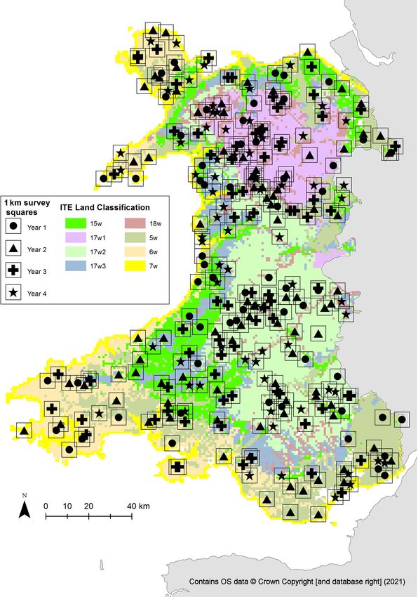
4156                                                             C. M. Wood et al.: Integrated ecological monitoring in Wales

          Landscape         features      (Maskell        et      al.,      2020a–c),     https://doi.org/10.5285/
       82c63533-529e-47b9-8e78-51b27028cc7f, https://doi.org/10.5285/9f8d9cc6-b552-4c8b-af09-e92743cdd3de,
       https://doi.org/10.5285/f481c6bf-5774-4df8-8776-c4d7bf059d40; Vegetation plots (Smart et al., 2020),
       https://doi.org/10.5285/71d3619c-4439-4c9e-84dc-3ca873d7f5cc; Topsoil physico-chemical properties
       (Robinson et al., 2019), https://doi.org/10.5285/0fa51dc6-1537-4ad6-9d06-e476c137ed09; Topsoil meso-
       fauna (Keith et al., 2019), https://doi.org/10.5285/1c5cf317-2f03-4fef-b060-9eccbb4d9c21; Topsoil particle
       size distribution (Lebron et al., 2020), https://doi.org/10.5285/d6c3cc3c-a7b7-48b2-9e61-d07454639656;
       Headwater       stream     quality   metrics     (Scarlett   et   al.,   2020a),   https://doi.org/10.5285/
       e305fa80-3d38-4576-beef-f6546fad5d45; Pond quality metrics (Scarlett et al., 2020b), https://doi.org/10.
       5285/687b38d3-2278-41a0-9317-2c7595d6b882; Insect pollinator and flower data (Botham et al., 2020),
       https://doi.org/10.5285/3c8f4e46-bf6c-4ea1-9340-571fede26ee8; and Bird counts (Siriwardena et al., 2020),
       https://doi.org/10.5285/31da0a94-62be-47b3-b76e-4bdef3037360.

1   Introduction                                                   1.1   Introduction to the GMEP survey design

The Welsh Government initiated the Glastir Monitoring and          While GMEP encompassed a range of different components,
Evaluation Programme (GMEP) in 2013 to evaluate the en-            including modelling and socio-economic surveys, a field
vironmental effects of the Glastir agri-environment scheme         survey formed the largest element of the monitoring pro-
at a national scale but also to monitor the wider country-         gramme. The field survey was designed in such a way as to
side of Wales (Emmett et al., 2015) in the longer term. In         capture multiple measures and metrics and to integrate across
Wales, funding from agri-environment schemes (AESs) has            these metrics. In order to do this, a full ecosystem-based ap-
been available since the early 1990s including Environmen-         proach was chosen such that data were captured across mul-
tally Sensitive Areas (ESAs), the Habitat Scheme, Wood-            tiple scales, where possible during a single field visit. A 4-
land Grant Scheme, Farm and Conservation grant scheme,             year cycle rolling survey was adopted in order to maximise
Tir Cymen, Tir Cynnal, Tir Gofal and most recently Gla-            the number of sites visited at the national scale, while also
stir. Currently, the Glastir scheme is the main method that        monitoring year on year. This would allow for cost-effective
the Welsh Government pays for environmental goods and              detection of both spatial variation and temporal trends (Em-
services (Emmett and GMEP team, 2014). The primary aim             mett and GMEP team, 2014). The first survey cycle dates
of GMEP monitoring was to collect evidence for the effec-          from 2013 to 2016, with the potential for, and intention of,
tiveness of bundles of management interventions in deliv-          regular repeat surveys.
ering outcomes of interest related to climate change mit-             Across GMEP monitoring, integration of survey data was
igation, biodiversity, soil and water quality, woodland ex-        a priority; therefore, a common spatial unit of 1 km for the
pansion, and cultural landscapes. Two additional objectives        survey square was adopted. A total of three-hundred 1 km
for reporting were added by the auditor general for Wales          survey squares (Fig. 1) were sampled over the 4-year cy-
in 2014: (1) to increase the level of investment in mea-           cle. The 1 km dimension was a conveniently sized unit for
sures for climate change adaptation, with the aim of build-        landscape monitoring, which has been adopted by previous
ing greater resilience to ongoing climate change into both         successful monitoring programmes. First tested for this type
farm and forest businesses and the wider Welsh economy,            of monitoring in a small scale survey in Cumbria (1975)
and (2) to use agri-environmental investment in a way that         (Bunce and Smith, 1978) and Shetland (1974) (Wood and
contributes towards farm and forest business profitability and     Bunce, 2016), the 1 km monitoring unit was later adopted for
the wider sustainability of the rural economy (Emmett and          the Countryside Survey of Great Britain from 1978 (Bunce,
GMEP team, 2017).                                                  1979) to present day and is used by other current monitor-
   The monitoring also collected evidence to quantify the          ing schemes, such as the Breeding Bird Survey (Harris et al.,
status and trends in the environment in general and con-           2018) and the Wider Countryside Butterfly Survey (Brereton
tributed to the The Second State of Natural Resources Report       et al., 2011). The 300 GMEP field-survey squares were split
(SoNaRR2020) (Natural Resources Wales, 2020). The data             evenly into two key components: the “Wider Wales Compo-
collected may be analysed in order to identify how drivers         nent”, used for baseline estimation, national trends and na-
of change, such as land use, climate and pollution affect the      tional reporting of Glastir, and the “Targeted Component”,
Welsh environment, beyond Glastir interventions (Emmett            which focussed on priority areas and aims of the Glastir
and GMEP team, 2014). This paper describes the key sets            scheme (Emmett and GMEP team, 2014).
of raw data arising from the field survey element of GMEP,            The Wider Wales Component of GMEP comprised one-
undertaken between 2013 and 2016.                                  hundred-and-fifty 1 km survey squares which were selected

Earth Syst. Sci. Data, 13, 4155–4173, 2021                                        https://doi.org/10.5194/essd-13-4155-2021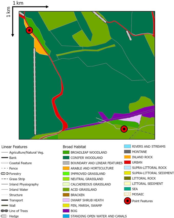
C. M. Wood et al.: Integrated ecological monitoring in Wales                                                                    4157

Figure 1. Map to show distribution of 1 km survey squares across different land classes in Wales (survey squares not shown to scale to
preserve data confidentiality).

following the same procedure as used for the UK Centre               mett and GMEP team, 2014). Land classes are derived from
for Ecology & Hydrology (UKCEH) Countryside Survey                   a statistical analysis of topographic, physiographic, geolog-
of Great Britain (Carey et al., 2008; Norton et al., 2012),          ical and climatic attributes. Environmental heterogeneity is
aiming to provide statistically robust estimates of indica-          minimised within each land class and is maximised between
tors from 1978 to 2016 at national and sub-national lev-             land classes. The number of 1 km survey squares randomly
els. Thus, “Wider Wales” squares were a stratified-random            sampled and sited from each land class was proportional to
sample of Wales, with proportional representation of strata          the area of that land class in Wales. This helped to optimise
defined according to the ITE Land Classification of Great            allocation of survey effort (Emmett et al., 2015).
Britain (henceforth “land classes”) (Bunce et al., 2007; Em-

https://doi.org/10.5194/essd-13-4155-2021                                            Earth Syst. Sci. Data, 13, 4155–4173, 2021
4158 C. M. Wood et al.: Integrated ecological monitoring in Wales
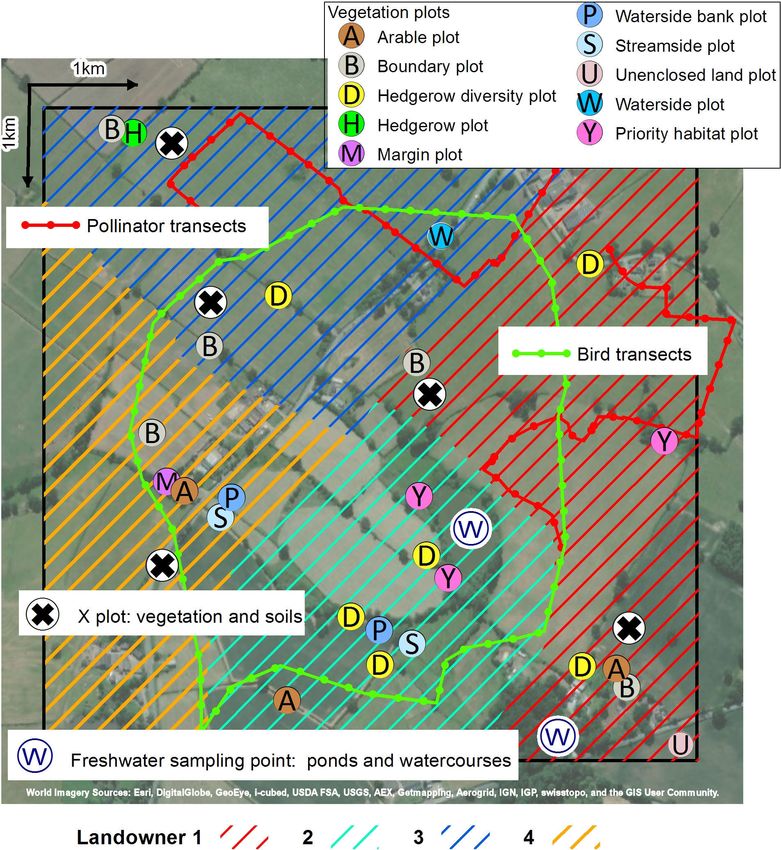
Figure 2. Type and distribution of published data collected in a
typical 1 km survey square (excluding the land cover and land use
mapping element; see Fig. 3) (Esri, 2021).
Figure 3. An example of a survey square, showing mapped point,
line and area features (the key includes the full range of possible
The other half of the sampled squares were targeted specif- broad habitats and linear features, not all shown on the map).
ically at Glastir priority areas (Welsh Government, 2020).
The squares were selected by calculating weights for each
1 km survey square across Wales that reflected the amount lished datasets, ancillary information was collected at survey
and diversity of Glastir uptake within the square (Emmett and sites regarding landscapes (photographs), footpath and his-
GMEP team, 2014). Squares were then randomly selected toric feature assessments.
with probability proportional to these assigned weights, such
that a square with twice the weight as another was twice as
likely to be selected. The weighting, and therefore selection 2.1 Land cover and land use
of Targeted Component squares, was repeated each year as The most geographically comprehensive element of the sur-
new information became available on Glastir uptake. Across vey is the mapping of land cover and ecologically relevant
both GMEP field-survey components, any square that con- landscape features (Fig. 3). The methods adopted were those
tained more than 75 % of urban land or that was more than of the UKCEH Countryside Survey, described in detail in
90 % sea (defined by the UK Land Cover Map 2007, Mor- Wood et al. (2018a). Across accessible areas of each 1 km
ton et al., 2011, and mean high tide data, Ordnance Survey, survey square, areal, linear and point features were mapped
2020) was excluded and replaced according to the above pro- digitally using Microsoft Windows 7-based electronic data
cedures (Emmett and GMEP team, 2014). capture equipment and electronic mapping software (“CS
Surveyor”) co-developed by the UK Centre for Ecology &
2 Data collected: field and laboratory collection Hydrology and software company, Esri UK (Maskell et al.,
methods 2008). With the aid of base maps, each feature was as-
signed a range of pre-determined coded attributes (Maskell
A wide range of data were collected during the field survey, et al., 2008; Wood et al., 2018a). For area features, at-
encompassing land use and cover, vegetation, soils, fresh- tributes for each mapped polygon included “biodiversity
waters, birds, and insect pollinators. Figure 2 illustrates the action plan” (BAP) broad/priority habitats (Jackson, 2000;
type and distribution of data collected in a typical 1 km sur- Maddock, 2008), land use and land management (for exam-
vey square, and a short summary of each of the elements ple, crop, grazing animals, recreation, timber, burning), dom-
is provided in this section. In addition to these key, pub- inant vegetation species, and a variety of other descriptors ac-
Earth Syst. Sci. Data, 13, 4155–4173, 2021 https://doi.org/10.5194/essd-13-4155-2021C. M. Wood et al.: Integrated ecological monitoring in Wales 4159
cording to the land use type (for example, road verge widths, were made to survey teams by managers, and difficult spec-
tree diameter at breast height, woodland structure, woodland imens could be collected and sent to experts for identifica-
features and sward descriptions) (Wood et al., 2018b). tion (Wood et al., 2017). A number of plots were repeated by
Linear features are landscape elements less than 5 m wide quality assessors to ensure consistency of quality within the
that form lines in the landscape (Wood et al., 2018b). Record- survey (Wood et al., 2017).
ing included the length and condition of a range of lin-
ear features predominantly, but not exclusively, describing 2.3 Soils
boundaries. These include managed woody linear features
(i.e. hedges), unmanaged woody linear features (i.e. lines Within each of the three-hundred 1 km sample squares, the
of trees), walls, fences, streams and a range of other linear key soil measurements described below were taken from a
features. Recorded linear features have a minimum length set of three volumetric topsoil samples (0–15 cm) sampled
of 20 m and may include gaps of up to 20 m (a rule agreed from each of five pre-determined randomly dispersed loca-
with hedgerow experts when compiling methods for UKCEH tions, using standard-sized plastic tubes and a metal cor-
Countryside Survey, Maskell, 2008). All linear features were ing implement. The sampling locations were coincident with
recorded unless they form part of a curtilage or they are the five large (“random”/“main”/“X”) vegetation plots (Ta-
within the woodland canopy. Woody linear features, includ- ble 1). Sampling started on the southern corner of the in-
ing hedges, remnant hedges and lines of trees were classified ner 2 × 2 m nest of the X plot in 2013 and then proceeded
using a key (Maskell et al., 2016a), following consultation west, north and east in the consecutive years. Soil samples
with the Hedgerow Steering Group of the UK BAP (Wood included one sample analysed for physico-chemical soil met-
et al., 2018b). rics, taken using a black plastic core (15 cm long × 5 cm di-
Point features are individual landscape elements that oc- ameter); a spare white core (15 cm long × 5 cm diameter);
cupy an area of less than 20 m × 20 m. Point features may and a sample for soil fauna (2013 and 2014), taken using a
be trees or groups of trees, ponds and other freshwater fea- shorter core (8 cm long). In 2013 and 2014, five bulked 0–
tures, physiographic features such as cliffs, buildings and 15 cm gouge auger samples for DNA metabarcoding were
other structures with various use codes (for example, “res- also taken and were frozen upon receipt at the laboratory un-
idential” or “agricultural”) (Wood et al., 2018b). For the de- til analysis. The methods for this area of work is outlined in
tailed methodology, see the GMEP field mapping handbooks George et al. (2019a). After collection, the soil cores were
(Maskell et al., 2016a, b). Quality assurance was achieved refrigerated and stored until posted, usually within 2 d, to
by ensuring surveyors were trained appropriately before each laboratories at the UK Centre for Ecology & Hydrology in
field season, visits to surveyors in the field by supervisors and Bangor and Lancaster for analysis and/or archive storage in
the repeat survey of a number of squares to identify any is- air-dried or frozen form.
sues arising.
2.3.1 Physico-chemical properties
2.2 Vegetation plots
The sample taken for analysing physico-chemical properties
The vegetation element of the field survey involved record- included measurements of the following properties: loss on
ing plant species presence and cover in different sizes and ignition (LOI) and derived carbon concentration, total soil
types of vegetation plot (Table 1), comprising different num- organic carbon (SOC) and nitrogen, total soil phosphorous,
bers of “nests” (i.e. subsections of the plot). The design of Olsen phosphorous, soil pH (in deionised water and calcium
the plots originated in the UKCEH Countryside Survey, and chloride), soil solution electrical conductivity, soil bulk den-
the history and logic behind their positioning is described sity of fine earth, fine earth volumetric water content (where
fully in Wood et al. (2017). A comprehensive description sampled), soil water repellency, and water drop penetration
of these plots may be found in the field survey handbook time. The methods for these are summarised in Table 2.
(Smart et al., 2016) with a summary presented in Table 1.
In each vegetation plot, a complete list of all vascular plants 2.3.2 Soil meso-fauna
and a selected range of readily identifiable bryophytes and
macro-lichens was made, with the exception of “D” (Diver- Soil meso-fauna were extracted using the standard Tullgren
sity) plots, in which only woody species in hedgerows were funnel method (Southwood, 1994), as used in the UKCEH
recorded (Wood et al., 2017). Cover estimates were made Countryside Survey (Emmett et al., 2008). Following the ex-
to the nearest 5 % for all species reaching at least an esti- traction procedure, the samples were sorted, identified and
mated 5 % cover. Presence was recorded if cover was less enumerated according to broad groups (as shown in Table 3)
than 5 %. Canopy cover of overhanging trees and shrubs was by trained staff and students (Emmett et al., 2008). These
also noted, alongside general information about the plot. To enumerated broad groups were entered into data template
ensure quality, the field training courses held before the sur- spreadsheets and, once complete, sent to UKCEH Bangor for
veys covered identification of difficult species, regular visits integration into the database.
https://doi.org/10.5194/essd-13-4155-2021 Earth Syst. Sci. Data, 13, 4155–4173, 20214160 C. M. Wood et al.: Integrated ecological monitoring in Wales
Table 1. Plot types included in GMEP (Smart et al., 2016).
Code Name Where Size No. per 1 km Additional information
survey square (sampling followed standard
protocols established by the
UKCEH Countryside Survey
https://countrysidesurvey.org.uk/,
last access: 13 August 2021, unless
stated below)
X Random/main/ Dispersed random points (not on linear 4 m2 Up to 5 In years 2013–2014, all X plots
X plot features). or 200 m2 were 200 m2 . In 2015–2016, due to
resource limitations, plots were re-
duced to 4 m2 (with the exception
of woodland habitats and a small
subset of squares).
Y Small: targeted Primarily allocated to “enclosed habi- 4 m2 Up to 5 but *
and tats” in or out of Glastir option and more if > 5 PH
enclosed/habitat then additionally placed to record prior-
ity habitats (PH) not sampled by other
plots.
U Unenclosed Unenclosed broad habitats in or out of 4 m2 Up to 10 *
Glastir options.
B Boundary Adjacent to field boundaries in or out 10 × 1 m 5 *
of Glastir option; randomly located in
relation to the X plot.
A Arable Arable field edges centred on each B 100 × 1 m Up to 5 *
plot; in or out of Glastir option but only
one per arable field; paired with X plots
if out of option.
M Margin Field margins in or out of Glastir op- 2×2m Up to 15 *
tion.
H Hedgerow Alongside hedgerows (i.e. woody linear 10 × 1 m 2
feature (WLF) with unnatural shape)
and usually coincident with two of the
D plots; randomly located in relation to
the X plots.
D Hedgerow WLF with natural or unnatural shape; 30 × 1 m Up to 10 *
diversity allocated proportionally to WLF in Gla-
stir option; randomly located in relation
to the X plots.
S/W Streamside Four placed alongside watercourses and 10 × 1 m Up to 5 *
allocated in proportion to Glastir option
uptake; one W plot centred on the river
habitat survey (RHS) stretch.
P Perpendicular Sampling the upslope habitats adjacent 10 × 1 m Up to 5 A new type of plot for the GMEP
streamside to and centred on the S/W plots. survey; nests within these plots are
of variable length, summing to 10 m
(Emmett et al., 2015).
R/V Roadside verge Sampling the 1 m strip adjacent to roads 10 × 1 m Up to 5 Only recorded in 2016, in a subset
plots and tracks. of squares.
∗ Location of these plots incorporated additional targeting to take into account the proportional amount of Glastir options in a 1 km survey square.
Earth Syst. Sci. Data, 13, 4155–4173, 2021 https://doi.org/10.5194/essd-13-4155-2021C. M. Wood et al.: Integrated ecological monitoring in Wales 4161 Table 2. Summary of soil physico-chemical properties and measurement methods. i. Loss on ignition Loss on ignition (LOI) is a simple and inexpensive method for determining soil organic matter and estimating soil organic carbon concentration. The method was the same standard method as that used in the UKCEH Countryside Survey (Emmett et al., 2010). LOI was measured on a 10 g air-dried sub-sample taken after sieving to 2 mm, then dried at 105 ◦ C for 16 h to remove moisture, weighed, and then combusted at 375 ◦ C for 16 h. The cooled sample was then weighed and the LOI (%) calculated (Emmett et al., 2010). In order to have data that were compatible with legacy data from other surveys, like UKCEH Countryside Survey, carbon (C) concentration was derived from the LOI measurement. Resulting C concentration measures, unlike those from some other methods, were thus unaffected by soil inorganic carbon. The formula for deriving C concentration is C concentration (g C kg−1 ) = LOI (%) · 0.55 · 10. LOI quality control checks were carried out using internal soil standards prepared in an identical manner to the sampled soils. Two different internal standards were included in each sample batch. Those internal standards were compared with a historically generated mean value for internal standards. If the measured LOI for the two internal standards in a batch varied by more than 2 standard deviations, in either direction, from the historic mean value, then the batch was repeated. ii. Total soil organic carbon (SOC) and nitrogen This analysis was carried out using the United Kingdom Accreditation Service (UKAS) accredited method SOP3102, at UKCEH Lancaster. Soil samples were air-dried (at 40 ◦ C), ball milled and oven-dried at 105 ◦ C (± 5 ◦ C) for a minimum of 3 h. Samples were then analysed using an Elementar Vario EL elemental analyser (Elementar Analysensysteme GmbH, Hanau, Germany), which is a fully automated analytical instrument working on the principle of oxidative combustion followed by thermal conductivity detection. Following combustion in the presence of excess oxygen, the oxides of nitrogen (N) and carbon (C) flow through a reduction column which removes excess oxygen. C is trapped on a column whilst N is carried to a detector. C is then released from the trap and detected separately. Sample weights are usually 15 mg for peat and 15–60 mg for mineral soil samples (Emmett et al., 2010). Quality control was achieved by use of two in-house reference materials analysed with each batch of samples. iii. Total soil phosphorous (P) Air-dried and ground (to 2 mm) soils were digested with hydrogen peroxide (100 volumes) and sulfuric acid in a 5 : 6 ratio. Selenium powder and lithium sulfate were added to raise the boiling point of the acid. Samples were then heated at 250 ◦ C for 15 min and then to 400 ◦ C where the temperature was maintained for 2 h to complete the digestion. After digestion, the samples were diluted with ultrapure water and allowed to settle overnight. The supernatant was then further diluted and P was measured colourimetrically using a SEAL AQ2 discrete analyser. Phosphorus was determined using ammo- nium molybdenum blue chemistry with the addition of ascorbic acid to control the colour production. Two quality controlled reference samples, a duplicate sample and two matrix matched blanks were run every 25 samples to ensure data quality. The final concentration (mg kg−1 ) was determined using a calibration curve of the standard and took into account the blank concentration. iv. Olsen phosphorous Olsen phosphorous was measured in samples from arable and improved grassland habitats only, where the measurement is most reliable (Emmett et al., 2010). Two grams of air-dried soil samples were extracted in 40 mL Olsen’s reagent (0.5 M NaHCO3 at pH 8.5) for 30 min in a mechanical end-over-end shaker. The sample was then filtered through a Whatman 44 filter paper to separate the soil and the filtrate; the filtrate is kept for analysis. The analysis was performed on a Seal Analytical AA3 segmented flow. The samples were mixed in the flow channel with an acidic ammonium molybdate and potassium antimony tartrate to form a complex with phosphate. This complex was reduced with ascorbic acid to develop a molybdenum blue colour. The reaction was temperature controlled to 40 ◦ C using a water bath to ensure uniform colour development. The developed colour was measured at 880 nm. Two quality controlled reference samples, a duplicate sample and two blanks were run every 25 samples to ensure data quality. The final concentration is expressed in milligrams per kilogram (mg kg−1 ) and is for moisture content, the concentration of the blank and using a calibration curve of the standard. v. Soil pH measurements in deionised water and calcium chloride (CaCl2 ) Soil pH was carried out on a suspension of fresh field-moist soil in deionised water and 0.01 M CaCl2 . The ratio of soil to water or CaCl2 was 1 : 2.5 by weight. The method used was based upon that employed by the Soil Survey of England and Wales (Avery and Bascomb, 1974). Two different internal standards were included in each sample batch for quality control. Batches in which the measured pH for the internal standards varied by more than 2 standard deviations in either direction from the mean value generated historically for the internal standards were repeated. https://doi.org/10.5194/essd-13-4155-2021 Earth Syst. Sci. Data, 13, 4155–4173, 2021
4162                                                                      C. M. Wood et al.: Integrated ecological monitoring in Wales

Table 2. Continued.

  vi. Soil solution electrical conductivity
  Ten grams of field-moist soil was weighed into a beaker with 25 mL of deionised water added and then stirred with a rod to produce a
  homogeneous suspension. After half an hour, the contents of the beaker were stirred again with the rod, and the electrical conductivity
  (EC) was measured using an electrode and a conductivity meter (Jenway 4510). For quality control, two different internal standards
  were included in each sample batch. Those internal standards were compared with a historically generated mean value for internal
  standards. If the measured EC for the two internal standards in a batch varied by more than 2 standard deviations, in either direction,
  from the historic mean value, then the batch was repeated.
  vii. Soil bulk density of fine earth and volumetric water content of fine earth
  The bulk density (BD) of soil depends greatly on the mineral make up of soil, soil organic matter and the degree of compaction. It
  is a measure of the amount of soil per unit volume and is therefore an excellent measure of available pore space in a soil, and gives
  information on the physical status of the soil. BD values are also essential when estimating soil C stocks, as they allow for a conversion
  from %C to C per unit volume. Bulk density was determined from a core which is 15 cm long with a diameter of 5 cm. Dry bulk density
  is calculated using the following equation:
                                 (Dry weight core (105 ◦ C) (g)−stone weight (g))
  Dry bulk density (g cm−3 ) =                      −3                     −3     .
                                  (Core volume (cm   )−stone volume (cm   ))
  viii. Fine earth volumetric water content when sampled
  Once the bulk density was calculated, the volumetric water content of the fine earth fraction could be determined by multiplying the
  bulk density and the gravimetric water content of the fine earth. Quality control was achieved by using fixed volume pre-cut sleeves for
  soil sampling and extensive training for soil surveyors.
  ix. Soil water repellency and water drop penetration time
  Soil water repellency (surface) measurement was carried out by measuring the time for a fixed volume droplet of deionised water
  (100 µL) to be fully absorbed into the soil surface (water drop penetration time, WDPT). Six drops of water were applied to an air-dried
  undisturbed soil surface. The entire process was filmed using a digital video camera so that the timing could be determined accurately.
  The samples were maintained in a laboratory at a relatively constant temperature ∼ 20 ◦ C. Some soils, especially arable, were not
  consolidated so measurements were taken on surface unconsolidated soil or aggregates using 20 g soil added to a tin lid and procedure
  followed as described above. For quality control, a micropipette was used to deliver the drops, six drops were used, and then the median
  value was obtained. All drop penetration measurements were captured using video, so times of penetration can be reviewed if required.

Table 3. Soil meso-fauna.

    Enumerated broad groups                               Details
    1    Acari           Oribatid – Phthiracaridae        Commonly known as “box” mites; these decomposers tend to be abundant in
                                                          woodlands.
    2                    Oribatid – others                Other oribatid mites, mostly decomposers or microbial feeders.
    3                    Mesostigmatid                    Predatory mites which feed on other soil meso-fauna.
    4                    Other                            Typically small mites; largely containing prostigmatids and juvenile mesostig-
                                                          matids.
    5    Collembola      Poduromorpha                     Podurid Collembolans; short legs and plump body shape.
    6                    Entomobryomorpha                 Entomobryid Collembolans; generally with long, slender body.
    7                    Symphypleona/Neelipleona         Symphypleonid Collembolans; small, round, globular body shape.
    8                    Total oribatids                  1+2
    9                    Total mites                      1+2+3+4
    10                   Total Collembolans               5+6+7
    11                   Total meso-fauna                 1+2+3+4+5+6+7

Earth Syst. Sci. Data, 13, 4155–4173, 2021                                                 https://doi.org/10.5194/essd-13-4155-2021
C. M. Wood et al.: Integrated ecological monitoring in Wales 4163
For the purpose of quality control, another member of staff 2.4 Freshwaters
checked 1 in 20 samples for the first 200 samples. Fauna
were then identified and enumerated by both members of A range of different types of data were collected from the
staff to ensure that the identification and counting procedures freshwater habitats of headwater streams and ponds. Data
employed by both individuals produced comparable results. were collected across the three-hundred 1 km survey sites,
This process was repeated at a reduced rate as the identifica- where the features occurred.
tions proceeded (Emmett et al., 2008).
2.4.1 Headwater streams
2.3.3 Particle size distribution (PSD) Data were collected from selected sections of headwater
The particle size distribution (PSD) of a soil, typically pre- streams, where present, in up to three-hundred 1 km squares
sented as the proportions of clay (< 2 µm), silt (2–63 µm) and according to standardised field methods (Kelly et al., 1998;
sand (63–2000 µm), is a fundamental property of the soil. It Murray-Bligh, 1999; O’Hare et al., 2013). Sampling points
controls nearly all edaphic processes and exerts strong con- were generally chosen to enable a full River Habitat Survey
trol on hydrology, transport of pollutants, availability of nu- (River Habitat Survey, 2021) to be taken in the square, while
trients, stabilisation of soil organic matter, mechanisms of also being as close as possible to an access point into the
erosion, gas exchange, soil biota and aboveground produc- square. Data relating to this freshwater element of the survey
tivity. The method of laser diffraction (LD) emerged in the are summarised in Table 4.
1980s as a potentially powerful tool for analysing granular
materials, and in the 1990s the soil science community began 2.4.2 Ponds
to apply LD to soils (e.g. Lebron et al., 1993). The method
has the advantage of being quick (about 5 min per sample), A bottled water sample was taken from a pond selected at
requires small amounts of soil (< 2.0 g), is reproducible and random from each 1 km survey site where present (a size con-
provides a wide range of size classes (rather than the conven- straint was used with a pond defined as “a body of standing
tional 3 to 9). water 25 m2 to 2 ha in area which usually holds water for at
For GMEP, particle size distribution was analysed in sam- least 4 months of the year”). The sample was sent to the lab-
ples with a loss on ignition lower than 50 % using a Beck- oratories at the UK Centre for Ecology & Hydrology, Lan-
man Coulter LS13 320 laser diffraction particle size analyser caster. The samples were analysed according to accredited
(Beckman Coulter Inc.) and the hydrometer method (Gee and methods as described for headwater streams in Table 4.
Or, 2002) (Emmett et al., 2015). Standard soil samples were To calculate pond biological quality, the method of the
included with each batch of samples, and duplicated sam- Freshwater Habitats Trust (Predictive SYstem for Multi-
ples were included (1 in 10) to check for reproducibility. metrics – PSYM) was used. This is a standardised method
To evaluate the accuracy of the instrument, different-sized (Howard, 2002) and is summarised as follows.
standards were used: nominal 500 µm glass beads (Beck- PSYM was developed to provide a method for assessing
man Coulter Inc.) and nominal 15 µm garnet (Beckman Coul- the biological quality of still waters in England and Wales.
ter Inc.). Sandy soil from Gleadthorpe (Cuckney, UK), clay The method uses a number of aquatic plant and invertebrate
soil from Brimstone (Denchworth, UK) and a silty soil from measures (known as metrics), which are combined together
Rosemaud (Bromyard, UK) were also used. All three soils to give a single value which represents the waterbody’s over-
are well-characterised farm soils from ADAS Ltd. In addi- all quality status (Williams et al., 1996). Using the method
tion, two well-characterised internal soil standards from the involves the following steps:
UKCEH laboratory were used (loam and silty clay loam).
1. Simple environmental data are gathered for each water-
The sand fraction was collected with a 63 µm sieve at the
body from map or field evidence (area, grid reference,
end of the drainage outlet. As a way to corroborate the laser
geology, etc.).
measurements, the weight of the sand collected in the sieve at
the end of the measurement was compared with the data pro- 2. Biological surveys of the plant and animal communities
vided by the instrument. In general, there was a good agree- are undertaken and net samples are processed.
ment for both values for the sand fraction. However, high
content of organic matter interference with the laser mea- 3. The biological and environmental data are entered into
surements was observed. After removal of organic matter, the PSYM computer programme, which
when the soil is very organic (loss on ignition (LOI) values
of 40 %–50 %), there are still some recalcitrant organic ma- i. uses the environmental data to predict which plants
terials that persist in the soil and produce overestimation of and animals should be present in the waterbody if it
the sand fraction measure with LD. is un-degraded and
ii. takes the real plant and animal lists and calculates a
number of metrics.
https://doi.org/10.5194/essd-13-4155-2021 Earth Syst. Sci. Data, 13, 4155–4173, 20214164 C. M. Wood et al.: Integrated ecological monitoring in Wales Table 4. Summary of freshwater properties and measurement methods. i. Diatoms Samples were digested using hydrogen peroxide to remove organic matter and mounted on slides using the mountant Naphrax. At least 300 valves on each slide were identified to the highest resolution possible using a Nikon BX40 microscope with 100× oil immersion objective with phase contrast. The primary floras and identification guides used were Krammer and Lange-Bertalot (1986, 2000, 1997, 2004), Hartley (1996) and Hofmann et al. (2011). All nomenclature was adjusted to that used by Whitton et al. (1998), which follows conventions in Round et al. (2007) and Fourtanier and Kociolek (1999). Members of the Achnanthidium minutissimum complex showed considerable morphological variability and were classified using the conventions in Potapova and Hamilton (2007). ii. Invertebrates Initially, samples were prepared by washing and sieving. Small portions of the samples were placed into a water filled sorting tray, marked with a grid to act as an aid, and systematically scanned for invertebrates. Examples of all taxa were placed into vials for quality assurance. After the first sort, the sample was then disturbed and/or rotated to expose previously hidden taxa. The process was repeated until all necessary taxa had been removed from the sample. Macroinvertebrates removed from the sample were identified to species level where possible, including Caddis and Diptera pupae but with the exception of Oligochaeta, Chironomidae, Simuliidae and Hydracarina. The majority of identification work was conducted using dissection microscopes with high-power microscopes used for examination of small specimens or specific parts of specimens. Terrestrial and aerial stages of aquatic species, terrestrial species and specimens which were dead when collected were not counted. Invertebrates which had become fragmented were only counted as a record if the thorax and abdomen were present. If only the posterior, abdomen or head was present, the species was not recorded. Though the abundances of taxa were not necessary for the Biological Monitoring Working Party (BMWP) water quality scoring system, they were recorded for use in other indices and environmental diagnostics. Only free-living individuals were counted. Colonies were counted as one individual. Very abundant taxa were recorded by distributing the sample evenly, counting the specimens in a portion of the tray using the grid lines and calculating the total by proportions. Quality control was carried out by the reanalysis of 1 randomly selected sample in every 20 by a different analyst. iii. Water chemistry Bottled water samples were sent to the laboratories at the UK Centre for Ecology & Hydrology, Lancaster, and were analysed according to accredited methods as described below: Phosphate (PO4 -P). PO4 -P concentrations were measured colourimetrically using a Seal Analytical AQ2 discrete analyser. PO4 -P was determined by re- action with acidic molybdate in the presence of antimony to form an antimony–phosphomolybdate complex. Ascorbic acid reduced this to the intensely blue phosphomolybdenum complex, measured spectrophotometrically at 880 nm. Calibration was produced by automatic dilution of a single stock solution of 0.2 mg L−1 PO4 -P; concentrations were obtained using the calibration curve within the range 0–0.2 mg L−1 . Control standards of 0.1 mg L−1 PO4 -P were analysed every 10 samples. Total dissolved nitrogen (TDN). A Skalar Formacs CA16 analyser with an attached ND25 filter was used to measure total dissolved nitrogen in water samples. TDN was measured by combustion at 900 ◦ C with a cobalt chromium catalyst which converts all nitrogen to nitric oxide. The nitric oxide was measured by a chemiluminescent reaction with ozone. The calibration range of the instrument was 0–4 mg L−1 for nitrogen. Samples with values over this range were diluted to within the range using 18.2 M carbon-free water. Alkalinity. Alkalinity was determined using a standard operating procedure for alkalinity in waters. Alkalinity was determined using the Mettler Toledo DL53 titrator, which performs analyses automatically using predefined methods. A complete titration method comprised sample dilution, dispensing of acid, stirring and waiting times, the actual titration, the calculation of results, and a report. Reagents and material used include standard buffer solutions from Fisher Scientific of pH 4 and pH 7, electrode filling solution made with potassium chloride solution (4 M) saturated with silver chloride from Fisher Scientific, 1.0 M hydrochloric acid, 0.02 M hydrochlo- ric acid, 1000 mg L−1 stock solution as calcium carbonate, 20 mg L−1 quality controlled standard as calcium carbonate, and deionised water. Alkalinity (usually) reflects the activity of calcium carbonate, so results were reported as milligrams per litre of calcium carbonate (mg L−1 CaCO3 ). Earth Syst. Sci. Data, 13, 4155–4173, 2021 https://doi.org/10.5194/essd-13-4155-2021
C. M. Wood et al.: Integrated ecological monitoring in Wales                                                                4165

   Finally the programme compares the predicted plant and         2.6   Pollinators
animal metrics with the real survey metrics to see how simi-
lar they are (i.e. how near the waterbody currently is to its     Each of the three-hundred 1 km survey squares was vis-
ideal/un-degraded state). The metric scores are then com-         ited twice (once each in July and August) in 1 year be-
bined to provide a single value which summarises the overall      tween 2013 and 2016. Butterfly Conservation (BC) subcon-
ecological quality of the waterbody. Where appropriate, in-       tracted nine experienced ecologists to survey 1 km survey
dividual metric scores can also be examined to help diagnose      squares across six regions of Wales (Emmett and GMEP
the causes of any observed degradation (e.g. eutrophication,      team, 2014). A further region was covered by a BC em-
metal contamination) (Williams et al., 1996).                     ployee. Pollinator surveys focused on three main pollina-
                                                                  tor groups: butterflies (Lepidoptera: Rhopalocera), bees (Hy-
2.5   Birds
                                                                  menoptera: Apoidea) and hoverflies (Diptera: Syrphidae).
                                                                  Butterflies were recorded to species level, whilst bees and
Bird surveys were coordinated by the British Trust for Or-        hoverflies were recorded as groups based on broad differ-
nithology (BTO). The survey protocol (Siriwardena and Tay-        ences in morphological features associated with ecological
lor, 2014) was designed to provide a robust estimate of the to-   differences. Note that training was critical for identification
tal numbers of breeding pairs of birds of each species found      of these groups, particularly hoverflies. In addition, the abun-
in each 1 km survey square and thus of change over time in        dance of common flowering plant groups (identified at the
future surveys, as well as information on the habitat patches     time of survey) was recorded using the DAFOR-X scale
in which individuals were recorded. Thus, the results provide     (D (dominant): > 30 %, A (abundant): 11 %–30 %, F (fre-
information on local abundance and the selection of habitat       quent): 6 %–10 %, O (occasional): 2 %–5 %, R (rare): 0 %–
types, such as areas under Glastir habitat management (Em-        1 %, X, not seen on route) (Emmett and GMEP team, 2014).
mett and GMEP team, 2014). The protocol operates at the              Survey visits were split into two independent parts: (1) a
same spatial scale as the national BTO/JNCC/RSPB Breed-           standardised 2 km transect route through each 1 km survey
ing Bird Survey (BBS) (Harris et al., 2019) but involves          square, established following the Wider Countryside Butter-
more intensive fieldwork, so it provides more accurate mea-       fly Survey (WCBS) method (Brereton et al., 2011; UKBMS,
sures of local abundance and is more appropriate for survey-      2020), which uses Pollard walks (Pollard, 1977), as used in
ing smaller samples of squares each year (60–90 vs. thou-         the UK Butterfly Monitoring Scheme (Brereton et al., 2019),
sands), with lower rates of repetition (Emmett and GMEP           and (2) a timed search in a 150 m2 flower-rich area within the
team, 2014). Measurement of habitat selection at the patch        square.
level also represents a finer scale of inference than is avail-      The transect route was split into two approximately paral-
able from the BBS, which aggregates birds and habitats at         lel 1 km routes separated by at least 500 m, and where pos-
the scale of the 200 m transect section. The field methods        sible at least 250 m in from the edge of the square. These
used thus incorporated elements of the BTO’s previous na-         routes were subdivided into ten 200 m sections. Flexibility
tional bird monitoring scheme, the Common Birds Census            in the route was allowed based on the presence of barri-
(O’Connor, 1990).                                                 ers such as roads and railways, urban areas, and refused ac-
   The surveys consisted of four (reduced to three from           cess permission. In each section the number of each butter-
2015–2016 onwards) visits to each square by trained, pro-         fly species and bee and hoverfly group within a 5 m2 record-
fessional BTO surveyors (Siriwardena et al., 2020). Surveys       ing box were recorded while walking the transect route at
were equally spaced through mid-March to mid-July. On             a steady pace. The DAFOR-X abundance of key flower-
each visit, the surveyor walked a route that passed within        ing plant groups (selected on the basis of being known to
50 m of all parts of the survey square to which access had        be important plant groups for pollinating insects) was also
been secured, beginning at around 06:00 (all times in this pa-    recorded within the 5 m2 recording box. At the end of the
per are given in local time) and taking up to 5 h. Surveys were   transect walk, the weather conditions were recorded: tem-
not conducted in conditions known to affect the detection of      perature (◦ C), sunshine (%) and wind speed (Beaufort scale)
birds, i.e. strong winds and more than light rain. The sur-       (Emmett and GMEP team, 2014).
vey route was started in different places on each visit so that      For the timed searches, surveyors identified a 150 m2
all areas were visited at least once before 08:00. All birds      flower-rich area within the 1 km survey square. In this area
seen or heard were recorded on high-resolution field maps         numbers of butterfly species and bee and hoverfly groups
using standard BTO activity codes. Recording and standard-        (the same groups as for the transect recording) seen within a
ising route coverage (where surveyors actually walked) was        20 min period were counted. Surveyors also recorded which
important both between visits and to ensure comparable re-        flowering plant group, if any, these pollinators were visiting.
peat coverage when squares are revisited (Siriwardena et al.,        Surveys were only conducted between 10:00 and 16:00 or
2020). The method is a distillation of the approach used for      between 09:30 and 16:30 if > 75 % of the survey area was
the BTO’s Common Birds Census between 1962 and 2000               un-shaded and weather conditions were suitable for insect
(O’Connor, 1990).                                                 activity. The criteria for suitable weather were temperature

https://doi.org/10.5194/essd-13-4155-2021                                        Earth Syst. Sci. Data, 13, 4155–4173, 2021
4166 C. M. Wood et al.: Integrated ecological monitoring in Wales
between 11 and 17 ◦ C with at least 60 % sunshine or above 2.9 Key findings as reported to Welsh Government
17 ◦ C, regardless of sunshine, and with a wind speed below 5
on the Beaufort scale (“small trees in leaf sway”) (Emmett Key findings were reported to the Welsh Government, along-
and GMEP team, 2014). side modelling and other outputs, in a 2017 report (Em-
mett and GMEP team, 2017) and online (https://www.gmep.
2.7 Quality assurance wales). A brief summary of some of these findings, as re-
ported in 2017, is presented as follows. In terms of biodiver-
In addition to specific measures already described for each sity and habitat condition of land in Wales, high-quality habi-
element, Department for Environment Food and Rural Af- tat plant indicator species (positive Common Standards Mon-
fairs (DEFRA) Joint Codes of Practice (JCoPR) were fol- itoring (CSM) species; JNCC, 2021) were found to be either
lowed throughout (DEFRA, 2015). The JCoPR sets out stan- stable or improving for arable, improved land, broadleaved
dards for the quality of science and the quality of research woodland and habitat land (land not in the former three cat-
processes. This helps ensure the aims and approaches of re- egories; mostly neutral grassland and upland habitat types).
search are robust. It also gives confidence that processes and The condition of blanket bogs is improving, as is the condi-
procedures used to gather and interpret the results of research tion of purple moor grass and rush pasture, which are two
are appropriate, rigorous, repeatable and auditable. priority habitats (Maddock, 2008). These habitats have been
The laboratories at the UK Centre for Ecology & Hy- targeted for improvement for many years, and many actions
drology (UKCEH), Lancaster, are UKAS (United Kingdom have been undertaken to support their recovery. The relative
Accreditation Service; https://www.ukas.com/, last access: importance of restoration practices, pollution reduction, cli-
13 August 2021) accredited. UKCEH maintains a qual- mate and/or rainfall changes still need to be explored. Initial
ity management system across its four sites which is ISO analysis also suggests a recent increase in the area of blanket
9001:2015 certified. bog and montane habitats (Emmett and GMEP team, 2017).
GMEP also identified a set of concerns in some national
2.8 Results to date trends. One such concern is the lack of woodland creation,
contrary to the ambitious targets of the Welsh Government
The data collected within the field survey have been anal-
(Emmett and GMEP team, 2017). While the mean patch size
ysed extensively, and the results and associated uncertain-
of habitat, including woodland, was found to have increased
ties are publicly available via GMEP (2021). One benefit of
over the last 30 years, no change was detected in the area
the structured sampling approach is that the “Wider Wales”
of small woodlands (< 0.5 ha). The small amount of area
control sample provides an unbiased national assessment of
planted within the Glastir scheme by 2017 (3923 ha) is within
stock and condition of common habitats including woodland,
the variability of the GMEP sample. Such small woodlands
soils, small streams and ponds. The same approach has been
are not currently captured by the National Forest Inventory
used for reporting on stock and condition of British ecosys-
(Forest Research, 2020) and are the woodlands most likely to
tems since 1978 by the UK Centre for Ecology & Hydrol-
be affected by Glastir (Emmett and GMEP team, 2017). This
ogy through the UKCEH Countryside Survey programme
does not appear to reflect the targets for expansion of wood-
(http://www.countrysidesurvey.org.uk/, last access: 13 Au-
lands set by the Welsh Government nor exploit the multiple
gust 2021) (Emmett and GMEP team, 2017). By following
benefits woodlands can bring for biodiversity, carbon seques-
the same approach for selecting sites and capturing data in
tration and water regulation. In fact, this lack of progress,
the field, GMEP results can be linked to past trends to put the
combined with increased agricultural activity, has led to an
current observations into context. This has many benefits for
increase in greenhouse gas emissions in Wales (Committee
interpretation of results. For example, a result of “no change”
on Climate Change, 2018). However, there has been an in-
(based on a comparison between GMEP and UKCEH Coun-
crease in plant species indicative of good condition in large
tryside Survey data) could be positive if it indicates a long-
broadleaved woodlands over the last 10 years, suggesting im-
term decline has now been halted, but it could be negative
proved management of existing sites (Emmett and GMEP
if a previously reported improvement was now stalled (Em-
team, 2017).
mett and GMEP team, 2017). The key results were reported
Regarding soils, topsoil carbon has been stable or has in-
to the Welsh Government as outlined below. Beyond this, ad-
creased in woodland and improved land soils over the last
ditional work has also been carried out in several areas. Re-
30 years. Across all land cover types, overall topsoil has be-
sults from the field survey are also complemented by outputs
come less acidic over the last 3 decades, with the most likely
from other parts of GMEP, such as modelling (for example,
reason being the large reductions of acidifying pollutants;
Emmet et al., 2017).
emission and deposition of acidifying pollutants across the
UK peaked in the 1970s. Recently, a small increase in the
acidity of topsoil in improved land has been observed. This
may be due to the long-standing decline in lime use com-
bined with continued fertiliser use. A recent loss of topsoil
Earth Syst. Sci. Data, 13, 4155–4173, 2021 https://doi.org/10.5194/essd-13-4155-2021C. M. Wood et al.: Integrated ecological monitoring in Wales 4167
carbon in habitat land has also been observed, driven pri- temporary National Plant Monitoring Scheme (Pescott et al.,
marily by a reduction in carbon concentration in acid grass- 2019). Similarly, GMEP pollinator surveys have provided a
land and heathland. This trend is currently being investigated national benchmark by which to assess the value of Wales’
further by UKCEH through targeted resampling of soils on salt marshes for bees (Davidson et al., 2020). More recently,
acid grassland and heathland sites (Emmett and GMEP team, GMEP data permitted the most comprehensive assessment of
2017). pollinator abundance across Wales’ habitats to date, reveal-
Concerning freshwaters, over the last 20 years, new analy- ing key roles for woodlands, woody linear features and crop-
ses of small stream data from Natural Resources Wales show lands (Alison et al., 2021). Maskell et al. (2019) combined
an ongoing improvement in invertebrate diversity and nutri- multiple strands of GMEP data to understand how species
ent status (Natural Resources Wales, 2016). GMEP sampling richness is distributed across landscapes, exploring relation-
of headwater streams indicates more than 80 % have high di- ships between land-use intensity, habitat heterogeneity and
versity according to invertebrate indicators. There are an esti- species richness of multiple taxa in order to map and moni-
mated 9500 to 16 000 km of headwater streams in Wales, and tor high nature value (HNV) farmland.
they are a priority conservation habitat for a range of charac- GMEP data have been used to investigate the quality and
teristic plant and animal species. In terms of livestock, 55 % value of landscapes in Wales as a whole, focusing on how
of small streams were found to be freely accessible. This in- different landscapes are valued by the public, as well as trans-
creases the risk of damage to banks and associated raised ferring the methods to landscapes in Iceland (Swetnam et al.,
sediment levels and increases the risk of phosphorus and 2017; Swetnam and Korenko, 2019; Swetnam and Tweed,
pathogen levels. The latter has implications for contamina- 2018). GMEP mapping data have also been used for accu-
tion of shellfish beds, human health and recreation. It should racy assessment of land cover maps, produced using satellite
be noted that some access for stock is essential for exposed- imagery (Carrasco et al., 2019).
river-sediment-specialist invertebrates (Emmett and GMEP A range of different work concerning soils has been un-
team, 2017). dertaken since 2016. This includes a consideration of differ-
Only 13 % of ponds sampled in GMEP were judged to ences in soil physico-chemical properties across habitats and
be in good ecological condition. Ponds are important to the relative to known thresholds for supporting habitat function
Welsh landscape, because they provide characteristic habi- (Seaton et al., 2020a). Several key soil properties, such as
tat and biota and support two-thirds of all freshwater species carbon, nitrogen and pH, were found to be strongly corre-
(Freshwater Habitat Trust, 2021). They act as stepping stones lated across soils and can be used to create a soils classifi-
for biota to disperse over wide distances while also providing cation. Soil analyses were complemented by microbiologi-
refuges for wildlife. They are also priority habitats under the cal measurements from DNA metabarcoding of specific tar-
EU habitats directive (Maddock, 2008). There is a substan- get genes, deposited with the European Nucleotide Archive
tial amount of pond habitat in Wales, around 57 800 ponds in (ENA) at EMBL-EBI (Environment Centre Wales (Bangor
total. Further analysis is needed to identify the cause of this University), 2016a–c). These results, and the methods used
poor condition which could include poor creation practice, to determine them are presented in George et al. (2019a),
lag time after pond creation, runoff from adjacent fields, etc. where it was demonstrated that soil microbial and soil ani-
Whilst pond numbers are high, their ecological value seems mal taxa respond differently to changes in land use and soil
in question considering the low number in good condition. type. Animal richness was governed by intensive land use
Better advice concerning their creation and management ap- and unaffected by soil properties, while microbial richness
pears to be needed (Emmett and GMEP team, 2017). was driven by environmental properties across land uses. The
efficacy of 18S and ITS1 barcodes in capturing fungal bio-
2.10 Additional published work to date
logical and functional diversity has been compared, revealing
barcode biases that influenced metrics of functional but not
The breadth and quantity of data available from the field biological diversity (George et al., 2019b). Investigations of
survey offers many opportunities for potential analyses, as bacterial functional groups in the 16S marker gene dataset
evidenced by work undertaken since the end of the field showed changes in sulfate-reducing bacterial communities
survey in 2016. Data have been used to investigate veg- across land uses, with highest richness in grasslands (George
etation species trends along linear features, incorporating et al., 2020).
GMEP data with those from the UKCEH Countryside Sur- Soil meso-fauna have been described by George et al.
vey 1990–2007 (Smart et al., 2017). Results indicated a con- (2017), explaining how broad soil meso-fauna groups dif-
tinuation of a trend towards increased shading and woody fered among disparate habitats, with abundances being low-
cover. Furthermore, data from GMEP vegetation quadrats est in arable sites overall, and Collembola and predatory
have been combined with plant trait databases and satellite mites being lower in uplands.
imagery to map net primary productivity across Wales (Tebbs In terms of soil particle size, soil textural heterogeneity
et al., 2017). GMEP vegetation data have also provided a na- was found to be positively linked to bacterial richness for
tional benchmark against which to assess bias in the con- the first time (Seaton et al., 2020b), but fungal richness was
https://doi.org/10.5194/essd-13-4155-2021 Earth Syst. Sci. Data, 13, 4155–4173, 2021You can also read