Dynamics of excited electronic states in functional materials - Diva Portal
←
→
Page content transcription
If your browser does not render page correctly, please read the page content below
Digital Comprehensive Summaries of Uppsala Dissertations
                from the Faculty of Science and Technology 2028

                Dynamics of excited electronic
                states in functional materials

                RAQUEL ESTEBAN-PUYUELO

    ACTA
UNIVERSITATIS
 UPSALIENSIS    ISSN 1651-6214
                ISBN 978-91-513-1179-1
  UPPSALA       urn:nbn:se:uu:diva-439069
    2021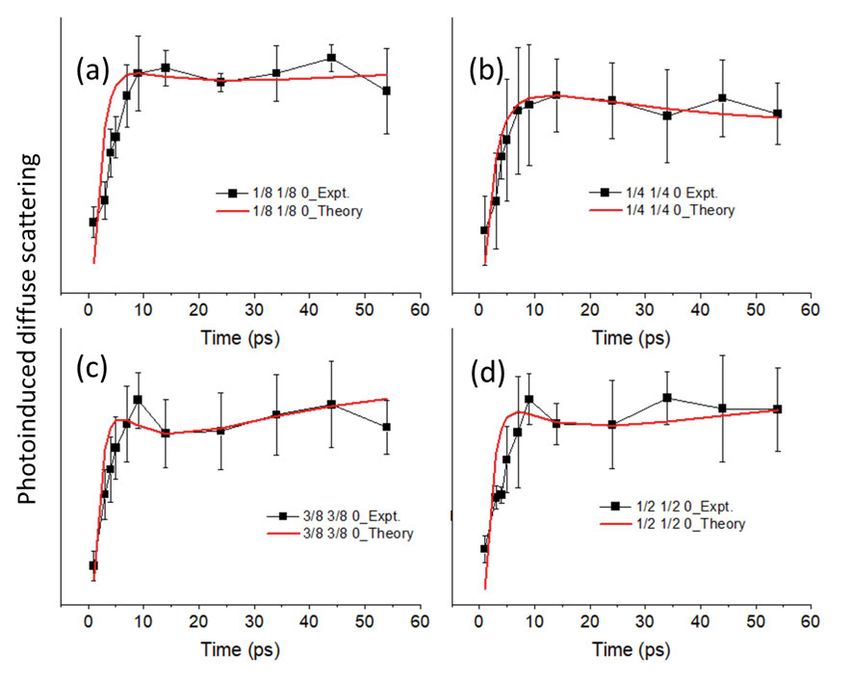
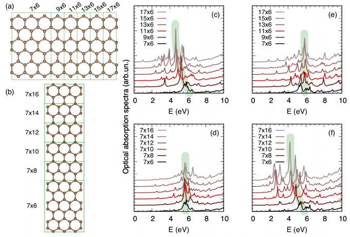
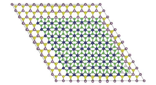
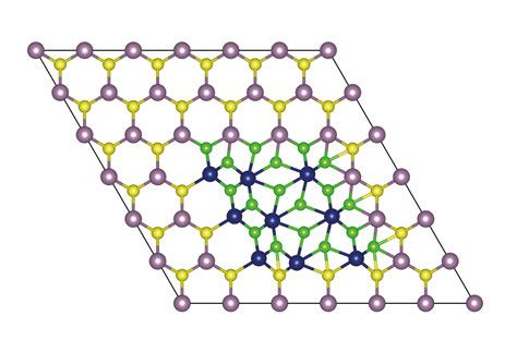
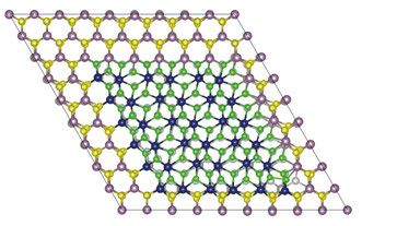
Dissertation presented at Uppsala University to be publicly examined in Häggsalen,
Ångströmlaboratoriet, Lägerhyddsvägen 1, Uppsala, Friday, 21 May 2021 at 09:15 for the
degree of Doctor of Philosophy. The examination will be conducted in English. Faculty
examiner: Patrik Rinke.

Abstract
Esteban-Puyuelo, R. 2021. Dynamics of excited electronic states in functional materials.
Digital Comprehensive Summaries of Uppsala Dissertations from the Faculty of Science and
Technology 2028. 77 pp. Uppsala: Acta Universitatis Upsaliensis. ISBN 978-91-513-1179-1.

Non-equilibrium processes involving excited electron states are very common in nature. This
work summarizes some of the theoretical developments available to study them in finite and ex-
tended systems. The focus lays in the class of Mixed Quantum-Classical methods that describe
electrons as quantum-mechanical particles but approximate ionic motion to behave classically.
In particular, Non-Adiabatic Molecular Dynamics and Real Time Density Functional Theory
are described and applied to answer questions regarding non-equilibrium dynamics in diverse
functional materials. First, the effect of phase boundaries and defects in monolayer MoS2 sam-
ples is studied. This material has been suggested as a good candidate to substitute silicon in
many applications, such as flexible electronics and solar cells. It is known that defects and dif-
ferent polymorphs are present in experimental samples, and therefore it is extremely important
to understand how realistic samples perform. We present how the electron-hole recombination
times are accelerated in presence of defects, as well as how the structural changes in sam-
ples that mix several phases of MoS2 affect their electronic structure. After that, rectangular
graphene nanoflakes are explored. As an application to finite systems, we show in rectangu-
lar graphene nanoflakes how different magnetic configurations have distinct optical absorption
spectra and how this can be used for opto-electronic applications. Furthermore, the high har-
monic generation for different magnetic couplings is studied, showing how some harmonics can
be suppressed or enhanced depending on the underlying electronic structure. Finally, dif-fuse
scattering in SnSe is investigated in an experimental collaboration in order to understand how
phonon-phonon interactions affect the scattering dynamics, which may lead to profound insight
into its thermoelectric properties.

Raquel Esteban-Puyuelo, Department of Physics and Astronomy, Materials Theory, Box 516,
Uppsala University, SE-751 20 Uppsala, Sweden.

© Raquel Esteban-Puyuelo 2021

ISSN 1651-6214
ISBN 978-91-513-1179-1
urn:nbn:se:uu:diva-439069 (http://urn.kb.se/resolve?urn=urn:nbn:se:uu:diva-439069)
A mi familia, aquí y allí
List of papers

This thesis is based on the following papers, which are referred to in the text
by their Roman numerals.

   I   Role of defects in ultrafast charge recombination in monolayer
       MoS2
       Raquel Esteban-Puyuelo and Biplab Sanyal
       arXiv:2103.13386 (2021), in revision in Phys. Rev. B

  II   Complexity of mixed allotropes of MoS2 unraveled by
       first-principles theory
       Raquel Esteban-Puyuelo, D.D. Sarma, and Biplab Sanyal
       Phys. Rev. B 102, 165412 (2020)

 III   Tailoring the opto-electronic response of graphene nanoflakes by
       size and shape optimization
       Raquel Esteban-Puyuelo, Rajat Kumar Sonkar, Bhalchandra Pujari,
       Oscar Grånäs, and Biplab Sanyal
       Phys. Chem. Chem. Phys., 22, 8212-8218 (2020)

 IV    Graphene nanoflakes as a testbed for electronic structure analysis
       through high harmonic generation
       Raquel Esteban-Puyuelo, Biplab Sanyal, and Oscar Grånäs
       Manuscript

  V Visualizing nonequlibrium atomic motion and energy transfer in
    SnSe
    Amit Kumar Prasad, Raquel Esteban-Puyuelo, Pablo Maldonado,
    Shaozheng Ji, Biplab Sanyal, Oscar Grånäs, and Jonas Weissenrieder
    Manuscript

Reprints were made with permission from the publishers.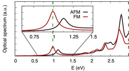
Comments on my contribution
Papers I-V are the result of close collaborations with the coauthors.

Paper I
I participated in the design of the project, performed all the calculations and
analysis and participated in discussions. I mainly wrote the manuscript and
handled its submission.

Paper II
I performed all the calculations and analysis. I participated in the discussions,
mainly wrote the paper and managed the replies to the referees.

Paper III
I participated in the design of the study and performed all the calculations (ex-
cept the NWChem benchmark done by RKS). I participated in the discussions
with the collaborators, mainly wrote the paper and managed the replies to the
referees.

Paper IV
Participated in the design of the project and performed the HHG calculations.
I contributed to the analysis of the results, and wrote the manuscript together
with OG.

Paper V
I performed the phonon and phonon-phonon simulations and participated in
the discussion, analysis and interpretations of the results. I contributed to the
writing of the manuscript.
Publications not included in this thesis

    Enhanced Gilbert damping in Re-doped FeCo films: Combined
     experimental and theoretical study
     Serkan Akansel, Ankit Kumar, Vijayaharan A. Venugopal,
     Raquel Esteban-Puyuelo, Rudra Banerjee, Carmine Autieri, Rimantas
     Brucas, Nilamani Behera, Mauricio A. Sortica, Daniel Primetzhofer,
     Swaraj Basu, Mark A. Gubbins, Biplab Sanyal, and Peter Svedlindh
     Phys. Rev. B 99, 174408 (2019)

    Structural phase transition in monolayer gold(I) telluride: From a
     room-temperature topological insulator to an auxetic
     semiconductor
     Xin Chen, Raquel Esteban-Puyuelo, Linyang Li, and Biplab Sanyal
     Phys. Rev. B 103, 075429 (2021)
Contents
1 Introduction ................................................................................................ 11
2 Theory and methods . . . . . . . . . . . . . . . . . . . . . . . . . . . . . . . . . . . . . . . . . . . . . . . . . . . . . . . . . . . . . . . . . . . . . . . . . . . . . . . . . . 13
2.1 Excited state dynamics . . . . . . . . . . . . . . . . . . . . . . . . . . . . . . . . . . . . . . . . . . . . . . . . . . . . . . . . . . . . . . . . . . 13
2.1.1 The full quantum problem . . . . . . . . . . . . . . . . . . . . . . . . . . . . . . . . . . . . . . . . . . . . . . 13
2.1.2 Mixed Quantum-Classical Dynamics: Non-Adiabatic
Molecular Dynamics . . . . . . . . . . . . . . . . . . . . . . . . . . . . . . . . . . . . . . . . . . . . . . . . . . . . . . . 15
2.2 The electronic system . . . . . . . . . . . . . . . . . . . . . . . . . . . . . . . . . . . . . . . . . . . . . . . . . . . . . . . . . . . . . . . . . . . . 20
2.2.1 Time-Dependent Density Functional Theory . . . . . . . . . . . . . . . . 21
2.2.2 Density Functional Theory . . . . . . . . . . . . . . . . . . . . . . . . . . . . . . . . . . . . . . . . . . . . . 25
2.2.3 Periodicity, basis sets and pseudopotentials . . . . . . . . . . . . . . . . . . 29
2.3 Non-equilibrium kinetic theory . . . . . . . . . . . . . . . . . . . . . . . . . . . . . . . . . . . . . . . . . . . . . . . . . . . . . 31
2.3.1 Phonons . . . . . . . . . . . . . . . . . . . . . . . . . . . . . . . . . . . . . . . . . . . . . . . . . . . . . . . . . . . . . . . . . . . . . . . . . . . . 31
2.3.2 Rate equations . . . . . . . . . . . . . . . . . . . . . . . . . . . . . . . . . . . . . . . . . . . . . . . . . . . . . . . . . . . . . . . . . . 34
3 Defect and interface induced phenomena in monolayer MoS2 . . . . . . . . . . . . . . 38
3.1 Summary of Paper I: Charge recombination . . . . . . . . . . . . . . . . . . . . . . . . . . . . . . . . 38
3.1.1 Ground state properties . . . . . . . . . . . . . . . . . . . . . . . . . . . . . . . . . . . . . . . . . . . . . . . . . . . 39
3.1.2 Non-adiabatic dynamics: electron-hole recombination 39
3.1.3 Conclusions of Paper I . . . . . . . . . . . . . . . . . . . . . . . . . . . . . . . . . . . . . . . . . . . . . . . . . . . . 42
3.2 Summary of Paper II: Coexistence of different phases . . . . . . . . . . . . . . . 43
3.2.1 Effect of strain in the band structures of the pure
phases . . . . . . . . . . . . . . . . . . . . . . . . . . . . . . . . . . . . . . . . . . . . . . . . . . . . . . . . . . . . . . . . . . . . . . . . . . . . . . . 43
3.2.2 Mixed phases: electronic structure . . . . . . . . . . . . . . . . . . . . . . . . . . . . . . . . . 44
3.2.3 Mixed phases: structural reconstruction . . . . . . . . . . . . . . . . . . . . . . . . 46
3.2.4 Conclusions of Paper II . . . . . . . . . . . . . . . . . . . . . . . . . . . . . . . . . . . . . . . . . . . . . . . . . . . 48
4 RT-TDDFT studies of graphene flakes . . . . . . . . . . . . . . . . . . . . . . . . . . . . . . . . . . . . . . . . . . . . . . . . . . . . . 50
4.1 Summary of Paper III. Shape and size dependent optical spectra
in magnetic GNF . . . . . . . . . . . . . . . . . . . . . . . . . . . . . . . . . . . . . . . . . . . . . . . . . . . . . . . . . . . . . . . . . . . . . . . . . . . . 50
4.1.1 Magnetism influences the optical spectra . . . . . . . . . . . . . . . . . . . . . . 50
4.1.2 Shape and size dependence on the optical spectra . . . . . . . . 52
4.1.3 Conclusions of Paper III . . . . . . . . . . . . . . . . . . . . . . . . . . . . . . . . . . . . . . . . . . . . . . . . . . 54
4.2 Summary of Paper IV: High harmonic generation . . . . . . . . . . . . . . . . . . . . . . 55
4.2.1 Calculation of the HHG spectrum . . . . . . . . . . . . . . . . . . . . . . . . . . . . . . . . . . 55
4.2.2 Harmonic yield dependency on the pulse duration and
the presence of resonances . . . . . . . . . . . . . . . . . . . . . . . . . . . . . . . . . . . . . . . . . . . . . . 564.2.3 Conclusions of Paper IV ................................................. 57
5 Diffuse scattering in SnSe . . . . . . . . . . . . . . . . . . . . . . . . . . . . . . . . . . . . . . . . . . . . . . . . . . . . . . . . . . . . . . . . . . . . . . . . . 58
5.1 Summary of Paper V . . . . . . . . . . . . . . . . . . . . . . . . . . . . . . . . . . . . . . . . . . . . . . . . . . . . . . . . . . . . . . . . . . . . . . 58
5.1.1 Ab initio simulations . . . . . . . . . . . . . . . . . . . . . . . . . . . . . . . . . . . . . . . . . . . . . . . . . . . . . . . . 58
5.1.2 Rate equations simulations . . . . . . . . . . . . . . . . . . . . . . . . . . . . . . . . . . . . . . . . . . . . . 59
5.2 Conclusions of Paper V . . . . . . . . . . . . . . . . . . . . . . . . . . . . . . . . . . . . . . . . . . . . . . . . . . . . . . . . . . . . . . . . . 60
6 Conclusions and Perspectives ................................................................... 62
Popular science summary ................................................................................ 64
Populärvetenskaplig samanfattning ................................................................ 66
Resumen divulgativo ....................................................................................... 68
Acknowledgements .......................................................................................... 70
References ........................................................................................................ 721. Introduction
Sólo el que sabe es libre, y más
libre el que más sabe.
(Only the one who knows is free,
and freer the one who knows
more)
Miguel de Unamuno
We have been using tools even since before we became humans. Choosing
natural materials and modifying them to suit our needs is a part of the devel-
opment of our species, and tools have been evolving accordingly from stone
knives to plastic bottles and mobile phones. We are surrounded by electronics:
from the simplest digital watch to the Perseverance Rover from NASA that is
exploring Mars, our world depends on efficient electronic devices. For more
than a century, they have been successfully made from bulk semiconductors
such as silicon, and they have become smaller with time. However, miniatur-
ization and improvement in efficiency have reached a plateau, since quantum
confinement and thermal losses play an important role when three-dimensional
structures reach a small enough size. One of the routes towards smaller scales
is to build devices made from two-dimensional materials, since their surface
area to volume ratio is maximal. Graphene, a single layer of graphite, has been
theoretically studied extensively since the 1950s [1] but not until its first ex-
perimental realization in 2004 [2], it became a promising alternative to silicon-
based electronics. Despite its extremely interesting properties (extraordinarily
high electron mobility and flexibility, to name a few), graphene is a semimetal,
and the corresponding lack of energy band gap limits its usage in semiconduc-
tor devices. One option to overcome this issue is to functionalize graphene
in order to open up a gap, for example by introducing defects [3] that modify
its electronic structure, or by creating nanoribbons and nanoflakes [4]. These
nanostructures are highly sensitive to size and shape due to quantum confine-
ment, and multiple efforts have been made to predict and characterize their
properties, for instance looking at their optical signatures. Another trend has
been the investigation of other 2D materials beyond graphene, either 2D al-
lotropes such as borophene, silicene, germanene, stanene, or compounds like
hexagonal boron nitride and transition metal dichalcogenides (TMDs) [5, 6].
TMDs are bulk materials composed of single layers bound together via weak
van der Waals forces, which can be exfoliated. MoS2 , one of the most studied
TMDs and an indirect band gap semiconductor of 1.29 eV in its bulk form,
11shifts to having a 1.8 eV direct gap in its most stable 2D phase. A direct gap is more efficient, which is why it is a promising candidate to substitute silicon in miniaturized electronic devices. Two-dimensional and bulk layered materials have been investigated with other applications in mind, and one of which is the exploitation of their capability to convert thermal into electrical energy. Thermoelectric materials such as SnSe [7, 8] lead a way into environmentally friendly power generation processes, and therefore studying their fundamental properties at the atomic scale is crucial for the development of this field. Many of the applications in which all these materials can be used are out of equilibrium. In fact, most of nature’s phenomena occur far from the ground state and are the response of a system after a perturbation. However, they have been historically tackled with methods that are within the Born-Oppenheimer approximation (decoupling of electron and ionic degrees of freedom), which is strictly valid only in the ground state and some particular transient situa- tions. The question of how to correctly study phenomena that involve excited electronic states has been around for a long time, and the quantum chemistry and experimental fields have done very important advances. Time-resolved experiments such as transient absorption spectroscopy are extensively used to study the relevant timescales and mechanisms [9], as well as excitonic prop- erties [10]. Very accurate theoretical solutions exist for small systems such as atoms and small molecules [11], but extended systems such as 2D mate- rials and bulk solids still pose a challenge. Many approximations need to be made, and the most important one is the neglect of the quantum nature of the ions composing the material. These groups of methods, in which ions are treated classically and electrons quantum-mechanically, are called semiclassi- cal methods and they are the basis of what will be discussed in this thesis. 12
2. Theory and methods

                                                  Why don’t you explain this to me
                                                  like I am five?
                                                                      Michael Scott

   The aim of this chapter is to provide a background on the theory and meth-
ods that serve as a basis for the projects that conform this thesis. I start in sec-
tion 2.1 with the full quantum mechanical description of the time-dependent
many-body problem, and then introduce the Mixed Quantum-Classical Dy-
namics by approximating the ionic motion as classical. I continue in section
2.2 by treating the electronic system in the effective framework given by Time-
Dependent Density Functional Theory, and finish the approximations path by
considering time-independent or ground state Density Functional Theory. Fur-
thermore, in section 2.3 I discuss lattice vibrations through the concept of
phonons, in order to introduce the rate equations that describe the transfer of
energy between the electronic and phononic system.
   Atomic units are used in this text unless otherwise stated (e2 =  = me = 1),
so distances are measured in Bohr and energies in Hartree.

2.1 Excited state dynamics
2.1.1 The full quantum problem
To exactly calculate time-dependent properties of an isolated non-relativistic
many-body system, one needs to solve the time-dependent Schrödinger equa-
tion (TDSE), which can be written as follows:
                              ∂ Ψ(R, r,t)
                          i               = HF Ψ(R, r,t).                     (2.1)
                                  ∂t
Ψ(R, r,t) is a short hand notation for the total wavefunction Ψ(r1 , r2 , ...rN ,
R1 , R2 , ...,t), which depends on the positions of the electrons {ri } and the
ions {RI }, as well as the time t. The full Hamiltonian operator is defined as

                  HF = Te + Tnuc +Ve−n +Ve−e +Vn−n +Vext .                    (2.2)

The first two terms in (2.2) are the kinetic energies of the electrons and ions,
the third term stands for the Coulomb interaction between electrons and ions,

                                                                                 13
the fourth and fifth terms represent the electron-electron and ion-ion interac-
tion and the last one is an external potential. More explicitly,
1 1 2 ZI
HF = − ∑ ∇2i − ∑ ∇I − ∑ +
2 i I 2mI i,I |ri − RI |
1 1 1 ZI ZJ
∑ + ∑
2 i= j |ri − r j | 2 I=J |RI − RJ |
+Vext , (2.3)
where mI is the mass of the Ith ion and ZI is the nuclear charge. Equation (2.3)
can be written in a more compact way grouping all terms except the nuclear
kinetic operator Tnuc into the electronic Hamiltonian:
HF = Tnuc + Hel . (2.4)
The total wavefunction can be exactly represented as a product of cou-
pled electron and nuclear wavefunctions without making any approximation,
through the Born-Huang/Born-Oppenheimer expansion:
Ψ(R, r,t) = ∑ ψ j (r)χ j (R,t) = ∑ ψ j (r; R)χ j (R,t). (2.5)
j j
ψ j (r) and χ j (R,t) are the electronic and nuclear wavefunctions in the dia-
batic representation, and ψ j (R, r) and χ j (R,t) are their counterparts in the
adiabatic representation.
The diabatic wavefunctions do not depend parametrically on the
nuclear po-
sitions and are typically defined to be orthogonal ψ j (r)ψk (r) = δ jk . This
means that when the diabatic expansion is inserted in (2.1), one can see that
the Hamiltonian matrix has only diagonal kinetic energy terms, and both di-
agonal and non-diagonal potential energy terms. The diagonal elements of the
potential
H j j (R) = ψ j (r) Hel ψ j (r) (2.6)
are the 3M-dimensional diabatic potential energy surfaces (PES), M being the
number of atoms.
On the other hand, in the adiabatic representation, the electrons follow the
static or time-independent Schrödinger equation
Hel ψ j (R, r) = E j (R)ψ j (R, r), (2.7)
so that ψ j (R, r) and E j (R) are the eigenfunctions and eigenvalues of Hel , re-
spectively. The adiabatic PES are then the functions E j (R). Choosing to
solve the TDSE in the adiabatic basis is very common because the electronic
wavefunctions are naturally orthogonal to each other (since they are eigen-
functions), so that they can directly form a basis. Furthermore, most of the
14electronic structure methods are written in the adiabatic basis, so it is conve-
nient. The nuclear wavefunction evolves following the TDSE, which in the
adiabatic basis can be expressed as
∂
[Tnuc + Ei (R)] χi (R,t) + ∑ Vi, j (R)χ j (R,t) = i χi (R,t). (2.8)
j ∂t
This was obtained by rotating the nuclear kinetic operator into the adiabatic
basis, or more explicitely, inserting the Born-Huang/Born-Oppenheimer ex-
pansion from (2.5) into (2.2) and multiplying by ψi∗ (r; R) from the left and
then integrating over the electronic degrees of freedom r. As mentioned be-
fore, Ei (R) are the adiabatic PES for the ith electronic state and the new term
resulting from the rotation, Vi, j (R), is the hopping term that allows transitions
between the ith and jth PES:
1 I
Vi, j (R) = − ∑ G (R) + 2di, j (R) · ∇I .
I
(2.9)
I 2mI i, j
GIi, j (R) = i| ∇2I | j is the scalar coupling vector in the braket notation and
dIi, j (R) = i| ∇I | j (2.10)
is the derivative coupling matrix, more often called nonadiabatic coupling
vector or NAC. It can be determined from the Hellman-Feynman theorem [12–
15]:
i| [∇I Hel (R)] | j − δi, j ∇I Ei (R)
dIi, j (R) = . (2.11)
E j (R) − Ei (R)
In some limiting cases, the electronic and nuclear degrees of freedom of the
total wavefunction can be factorized into a single product. One of these cases
is what is called the Born-Oppenheimer approximation [16]. In the adiabatic
representation, this is translated into assuming that the NACs can be ignored
in (2.8). The expression in (2.11) can give us a hint of when this is a good ap-
proximation. For instance, if the energy difference in the denominator is too
large (the PES are very far from each other) then the NACs can be neglected.
Additionally, the numerator scales as a force term, so if the force on the nu-
clei is small enough (the nuclei are moving slowly enough compared to the
electrons) the NACs play a negligible role.
A visual representation of the full quantum dynamics corresponding the
exact solution to a problem beyond the Born-Oppenheimer approximation in
the adiabatic representation is shown in figure 2.1.
2.1.2 Mixed Quantum-Classical Dynamics: Non-Adiabatic
Molecular Dynamics
In the Born-Oppenheimer approximation, the nuclear wavefunction propa-
gates adiabatically on a single PES. Since this is not a good approximation
15
Figure 2.1. Schematic illustration of the full quantum dynamics. The initial wave-
function propagates in the adiabatic excited state PES S1 and the final wavefunction
is a superposition of states in S1 and the ground state PES S0 after passing through
region with a high NAC. The horizontal axis indicates a general reaction coordinate.

for many time-dependent problems of interest, we need methods that go be-
yond the Born-Oppenheimer approximation, which is what methods like the
ones encompassed in the term Non-Adiabatic Molecular Dynamics (NA-MD)
do. Since solving numerically the nuclear TDSE scales exponentially with the
dimension of the problem, it is limited to very small molecules of less than 5
atoms. There are several ways of reducing the dimensionality by selecting the
important vibrational modes which are relevant for the problem, which can
allow for slightly bigger molecules, but approximations need to be made for
larger systems.
   The mixed quantum-classical dynamics retains the quantum nature of the
electrons but makes the approximation that the nuclear degrees of freedom
can be described classically. The classical equations of motion scale linearly
with dimension (instead of exponentially), which reduces the complexity of
the problem substantially. The multiple spawning, and specially Ehrenfest
and surface hopping approaches, described in the following subsections, are
the most popular mixed quantum-classical methods and have been applied to
a very long list of materials and phenomena. More information about these
methods can be found in these extensive reviews [17–20].

Ehrenfest dynamics
The Ehrenfest method is a mean field approach that considers that the elec-
tronic and nuclear wavefunctions in (2.5) are uncorrelated:

                     Ψ(R, r,t) = χ0 (R,t) ∑ c j (t)ψ j (R, r).               (2.12)
                                             j

χ0 is a single Gaussian function (which is assumed to be highly localized
in space) and the c j (t) are complex coefficients. According to the Ehrenfest

16
theorem the Newtonian laws are satisfied for mean values in quantum systems
with momentum p, mass m and under a potential V :
d r p d p
= and = ∇V . (2.13)
dt m dt
By using the Ehrenfest theorem and making the local approximation of Hel one
arrives to the equations of motion for the time-dependent nuclear quantities,
positions R and momenta P:
∂R P
= Ψ| i [Hel , R] |Ψ =
∂t M
∂P
= Ψ| i [Hel , −i∇] |Ψ = Ψ| ∇Hel (R) |Ψ . (2.14)
∂t
[A, B] is the commutator of A and B, and M is the mass of the nucleus. In
summary, in Ehrenfest dynamics the nuclei move in a single average PES, as
figure 2.2 shows.
Figure 2.2. Schematic illustration of the Ehrenfest dynamics. Trajectories run on a
mean field PES averaged over all the electronic states, weighted by their electronic
population. The horizontal axis indicates a general reaction coordinate.
It is interesting to note that the forces on the nuclei are averaged over many
adiabatic electronic states influenced by the nuclear motion and have the fol-
lowing form:
∂
FEhrenfest = Ψ| Hel |Ψ . (2.15)
∂r
This expression should not be confused with the Hellman-Feynman forces that
are calculated in ground state methods
∂
FGS = Ψ Hel Ψ , (2.16)
∂r
17where the partial derivative can be moved inside the expectation value because
it is a stationary case, unlike in (2.15).
One of the major assumptions taken in this method is that the nuclear wave-
function can be represented by a single Gaussian function, instead of a sum of
Gaussians or more accurate functions. This, combined with the classical treat-
ment of the trajectory, results in branching of the wavefunction not being pos-
sible, which would be allowed if the nuclear degrees of freedom were treated
fully quantum mechanically. Furthermore, this method is overcoherent, which
means that it is unable to describe the decoherence of electronic states, result-
ing in long-lived electronic excitations. However, Ehrenfest dynamics is able
to appropriately describe systems in which the nuclei are heavy and the range
of motion is small, and the electron-nuclear correlations are minimal. It has
been successfully applied to nanostructures, big molecules and other extended
systems to study processes that do not conserve energy.
Surface Hopping
In order to have a better description of the electron-nuclear correlation in
Eherenfest dynamics, Tully developed a surface hopping (SH) scheme based
on Molecular Dynamics (MD) [21]. In this family of methods, the nuclear
trajectory evolves in a single adiabatic electronic PES but is allowed to hop to
another surface, which is dictated by a probability, as figure 2.3 shows. The
main idea behind SH methods is to approximately recover the quantum be-
haviour of the nuclear trajectories by calculating multiple events of the same
trajectory, which, given the randomness included in the probability, generate
different outcomes.
Figure 2.3. Schematic illustration of the SH methods. An ensemble of trajectories
are propagated on the adiabatic BO PES and jumps are allowed between them. The
horizontal axis indicates a general reaction coordinate.
The most broadly used SH method is the Fewest Switches Surface Hop-
ping (FSSH), in which the population balance is maintained with the mini-
mum amount of hops possible. In its most popular implementation, the nu-
18clear system is treated classically via ab initio MD and the electronic wave-
function ψ(r, R,t) is represented in the basis of adiabatic electronic functions
φ (r; R(t)). They can be taken as Kohn-Sham (KS) orbitals if DFT is the
method of choice, as in the following expression:
ψ(r, R,t) = ∑ ci (t)φi (r; R(t)). (2.17)
i
The ci are the time-dependent expansion coefficients, and their evolution is
governed by a TDSE, which can be expressed as follows:
dci
i = ∑ (εi δi j − idi j ) c j . (2.18)
dt j
εi is the diagonal part of the electron Hamiltonian and the off-diagonal di j
represent the NAC have already been defined in (2.10). The probability for
the transition from an electronic state |i to a new state | j in a small time
interval Δt = t = t can be expressed as
gi→ j (t) = max (0, Pi→ j (t)) (2.19)
with
Re c∗i (t )c j (t ) M
P
di j (t)
Pi→ j (t) ≈ 2 ∗
. (2.20)
ci (t )c j (t )
These probabilities are compared to a uniformly distributed random number
to determine if the system is to remain in the current PES or hop to the next
one and nuclear velocities are rescaled to maintain the total energy. If that
rescaling is not possible then the hop is rejected.
In the original FSSH, the nuclear and electronic degrees of freedom are
completely coupled, so everything is updated on the fly at each time step.
However, the Classical Path Approximation (CPA) [22] can be used to further
reduce the computational cost by making the approximation that the classical
trajectory of the nuclei is independent of the electronic dynamics but the elec-
tronic dynamics still depends on the nuclear positions. In practice, this means
that the electronic problem can be solved on a series of pre-computed nuclear
trajectories, typically from ab initio MD. Since the feedback from the elec-
trons is not taken into account, this approximation is not valid if the electron-
nuclear correlations are crucial, such as in small systems like molecules. How-
ever, it is expected to produce reasonably good results for extended solids and
it is currently the most widespread method to tackle solid-state systems. In
FSSH-CPA, the hop rejection and velocity rescaling from (2.19) become
gi→ j (t) −→ gi→ j (t)bi→ j (t), (2.21)
19where the probability is scaled by a Boltzmann factor to account for the fact
that transitions to states high up in energy are less probable:
E −E −ω
exp − j kBiT if E j > Ei + ω
bi→ j (t) (2.22)
1 if E j ≤ Ei + ω.
Here kB is the Boltzmann constant, T is the temperature, and ω is the energy
of the absorbed photon in case of light-matter interaction, where has been
included for clarity.
Same as with Ehrenfest dynamics, by having a classical description of the
nuclei, we miss the loss of quantum coherence within the electronic subsys-
tem that is induced by the interaction with the quantum-mechanical vibra-
tions. Surface hopping can develop non-physical coherences and this is why
decoherence-induced surface hopping (DISH) was developed. It accounts for
the branching of nuclear trajectories by allowing hops at the decoherence times
only, which are calculated within the optical response theory using the auto-
correlation function of the fluctuation of the energy gap between two electron
states, as described in [23].
Multiple Spawning
In the last MQCD method that I will discuss here, the Multiple Spawning
(MS) method, the nuclear wavefunctions are expanded as a linear combina-
tion of Gaussian functions that are propagated classically. It is common to
refer to it as ab initio Multiple Spawning when it is connected to an electronic
structure method. The main difference between MS and the previously de-
scribed methods is that the number of nuclear functions is not a constant, and
each function is allowed to bifurcate and produce two functions in regions of
the PES landscape in which the NACs are large, as figure 2.4 shows. These
are called spawning events and give name to the method.
In the theoretical case of an infinite basis, the MS is an exact theory, in
opposition to both SH and Ehrenfest dynamics. However, since the NACs
need to be calculated at each time step and the basis of the nuclear functions
can be large, MS is computationally very expensive. Therefore, compromises
need to be made to truncate the basis as well as making local approximations
to compute integrals, which reduces the applicability of MS on large systems
or long timescales, in favour of less accurate but more practical methods like
Ehrenfest or SH.
2.2 The electronic system
So far I have discussed how to treat the coupling between the electronic and
ionic degrees of freedom. In this chapter I will focus on the quantum-mechanical
approach to the electronic system, introducing an effective density framework
20
Figure 2.4. Schematic illustration of the MS method. Classical trajectories are repre-
sented by single Gaussian functions. After the high NAC region, multiple Gaussians
can be created in different PES than the original. The horizontal axis indicates a gen-
eral reaction coordinate.

that reduces the degrees of freedom of the problem making it tractable. I will
first describe the general time-dependent case with Time-Dependent Density
Functional Theory (TDDFT) and then I will consider the special case of time-
independent or ground state Density Functional Theory (DFT).

2.2.1 Time-Dependent Density Functional Theory
I will start by assuming that the electronic system is non-adiabatic. We can
think about approaching the problem directly by solving the time-dependent
Schrödinger equation, but this is even more difficult than for the ground state
(which I will develop in 2.2.2) and it becomes extremely computationally ex-
pensive as the number of electron grows. However, inspired by ground state
DFT, we can try to develop a time-dependent DFT in order to reduce the num-
ber of variables in our problem. We will see in this section that Runge and
Gross proved the time-dependent equivalent of the KS theorem and I will give
an overview on the basics of TDDFT.

One-to-one correspondence and Time-Dependent Kohn-Sham equations
The evolution of the wavefunction describing N interacting electrons is given
by the time-dependent Schrödinger equation, which I have already shown in
(2.1) but choose to include here for clarity:
                            ∂ Ψ(R, r,t)
                              i          = H Ψ(R, r,t).                        (2.23)
                                 ∂t
Since it is a first-order differential equation in time, it needs an initial condition
from the wavefunction at time 0 (Ψ(t = 0)). The Hamiltonian operator is
                                  H = Te +Ve−e +Vext (t),                       (2.24)

                                                                                    21
where I have now grouped in Vext (t) the potential the electrons experience due
to the nuclear attraction as well as any external potential applied to the system.
In general, it is a sum over all the electrons
N
Vext = ∑ vext (ri ,t). (2.25)
i=1
The electron density (normalized to the number of electrons N) is given by
n(r,t) = N d 3 r2 . . . d3 rN |Ψ(r1 , r2 . . . rN ,t)|2 (2.26)
and evolves with time from an initial point t = 0. Runge and Gross proved an
analog of the Hohenberg-Kohn theorem for time-dependent systems in what is
called the one-to-one correspondence [24]. This theorem, central in TDDFT,
states that the densities n(r,t) and n (r,t) evolving from the same initial state
Ψ(t = 0) under the influence of two potentials vext (r,t) and vext (r,t) that are
Taylor expandable around t = 0 will eventually differ if the potentials differ
by more than a purely time-dependent function:
Δvext (r,t) = vext (r,t) − vext (r,t) = c(t). (2.27)
What this means is that there is a one-to-one correspondence between one-
electron densities and potentials. This implies that we only need to know
the time-dependent density of a system evolving from a given initial state to
uniquely identify the potential that produced that density. The potential in its
turn completely determines the Hamiltonian, so (2.23) can be solved to obtain
all the properties of the system.
Now, knowing that finding functionals of the density is a difficult task, I will
turn to the Kohn-Sham system, a fictitious system of non-interacting electrons
that reproduce the density of the interacting electrons. All the real properties
can be obtained from the effective density of the KS system, which is time-
dependent:
N 2
ne f f (r,t) = ∑ φ j (r,t) . (2.28)
j=1
The KS orbitals φ evolve according to the time-dependent KS equation:
∂ ∇2
i φ j (r,t) = − + vKS ne f f ; ψ(0) (r,t) φ j (r,t). (2.29)
∂t 2
This vKS (parametrically dependent on the initial state) is unique and can be
decomposed in three terms:
vKS ne f f ; Ψ (r,t) = vext (r,t) + vH (r,t) + vxc (r,t). (2.30)
22vH (r,t) is the usual Hartree potential and the exchange-correlation potential
vxc (r,t) is a very complicated quantity, even more than in the ground state
because it is a functional of the entire history of the density, the initial inter-
acting wavefunction ψ(0) and the initial KS wavefunction φ (0). In ground
state DFT, the exchange-correlation potential is the functional derivative of
the exchange-correlation energy, which is not so simple in TDDFT. A first at-
tempt to deal with time-dependent exchange-correlation functionals is to use
the Adiabatic Local Density Approximation (ALDA), even if it neglects all
nonlocality in time. More sophisticated functionals with memory effects have
been proposed [25–27].
Response functions and time-propagation in TDDFT
Many interesting physical quantities are the reaction of a system to an external
perturbation and can be expressed as a response function. More explicitly, if
an external field F is applied to a many-electron system, the system responds
and this can be measured as a change in a physical observable P as a functional
of F:
ΔP = ΔPF [F]. (2.31)
Its exact form can be very complex, but if F is weak, the response can be
written as a power series of the field strength. The first order response is called
the linear response of the observable. For example, the first order response of
the dipole moment to an external electric field is the polarizability and the first
order response of a magnetic moment to a homogeneous magnetic field is the
magnetic susceptibility.
There are different methods to calculate response functions from TDDFT:
real time propagation (RT-TDDFT), Sternheimer [28, 29], and Cassida meth-
ods [30]. Here I am going to focus on the first one, which consists of propa-
gating the electronic density in real time according to the TD-KS equation in
(2.29) using the so-called adiabatic approximation. Therefore, the KS Hamil-
tonian is a functional of the instantaneous density, not the whole history. If no
perturbation is present, the evolution of the KS wavefunction is
φ j (t) = φ j (0)e−iε j (0)t , (2.32)
where ε j is the eigenvalue of the jth KS wavefunction. However, if there is an
applied time-dependent perturbation with a frequency ω and a strength λ of
the general form
vext (r,t) = λ (r) cos(ωt) + λ (r) sin(ωt), (2.33)
then we can obtain the evolution of the wavefunctions from (2.29) and thus all
the response functions. For instance, we can calculate the dielectric properties
of our systems with RT-TDDFT by studying its dynamical response to the per-
turbation created by a weak external electric field by monitoring the evolution
23of the electrical dipole moment p j,k , which is calculated through
p j,k (t) = Tr Dk n(t) , (2.34)
where j and k indicate the directions of the applied field and measurement
respectively, and the transition dipole tensor operator is defined as
Dkμν = ϕμ |êk · r| ϕν , (2.35)
where ϕ are the basis functions in the electronic structure method of choice.
D is related to the polarizability tensor α(t) by
t
p j,k (t) = α j,k (t − t )E j (t )dt , (2.36)
−∞
with E j being the jth spatial component of the external electric field. If we
apply an instantaneous delta pulse
E(t) = E0 δ (t − t0 )ê j , (2.37)
it yields the following after Fourier transforming:
p j,k (ω)
α j,k (ω) = . (2.38)
E0
The absorption cross section can be obtained via
4πω
σ j,k (ω) = Im α j,k (ω) , (2.39)
c
which leads to the optical absorption spectra (strength function)
1
S(ω) = Tr [σ (ω)] . (2.40)
3
In RT-TDDFT higher-order responses (hyperpolarizabilities) are included.
The linear response regime can be achieved by applying a weak enough elec-
tric field, as the nonlinear contributions to the response function will be neg-
ligible. This capability of RT-TDDFT to explore phenomena that go beyond
the first, second or third order in perturbation theory result in it being a great
tool to study phenomena such as High Harmonic Generation (HHG). HHG is
the process by which a target system is illuminated with a laser frequency of
a certain frequency ω and it emits light in frequencies that are multiples of ω
(harmonics), as figure 2.5 presents.
HHG is relatively well understood for atoms and small molecules [31, 32],
but its fundamentals are still under discussion for extended systems such as
solids, monolayers and large molecules [33–37]. Many theoretical studies
rely on perturbation theory and therefore are limited to the second or third
24Figure 2.5. Schematic illustration of the high harmonic generation in a graphene flake.
The red wave indicates the incoming laser, the outgoing waves are the high harmonics
generated by the target.
harmonic order [38], and the few that use RT-TDDFT, although they report a
good matching with experiments, are quite inconclusive in terms of giving an
explanation for the mechanisms behind the phenomenon [39–41].
There is currently a discussion whether the spectral function S(ω) is pro-
portional to the dipole, its velocity or its acceleration. It has been shown that
for an atomic system, the HHG response is proportional to the dipole veloc-
ity [42]:
1
S(ω) = | ṗ(ω)|2 . (2.41)
4ε02 c2
Therefore, because RT-TDDFT provides the dipole in the time domain, the
HHG spectra is calculated as the following Fourier transform of its velocity:
2
HHG j,k (ω) ∝ FT ṗ j,k (t) . (2.42)
2.2.2 Density Functional Theory
I will now consider a special case: if the time-dependence of the ionic sys-
tem influences the electronic system only through the Born-Oppenheimer ap-
proximation and there are no external fields that give a time dependency to
the Hamiltonian, then the first order differential equation (TDSE) can have a
time-independent solution multiplied by an integrating factor that carries the
time-dependency. This is exactly what the Born-Oppenheimer approximation
means in practice, that we can solve the electronic problem in each snapshot
of frozen ions. Therefore, we can focus on the time-independent part of the
problem and discuss Density Functional Theory (DFT).
25With all these considerations, the wavefunction can be written as a sim-
ple product of time-dependent and time-independent parts, which leads to the
time-independent Schrödinger equation:
H Ψ(r1 , r2 , ...rN , R1 , R2 , ...) = EΨ(r1 , r2 , ...rN , R1 , R2 , ...). (2.43)
Equation (2.43) can only be solved exactly for the case of the hydrogen
atom, and approximations need to be introduced already for the helium atom,
which has 3 particles. If we restrict ourselves to stationary or ground state
properties, the already introduced Born-Oppenheimer approximation can be
used relying on the fact that the ions are much heavier than electrons and
therefore can be considered as frozen, so that they become a static term in the
external potential that the electrons feel. Within the BO approximation, the
electronic Hamiltonian has a simpler expression:
1 ZI 1 1
H =− ∑ ∇2i − ∑ + ∑ . (2.44)
2 i i,I |ri − RI | 2 i= j |ri − r j |
Even with this approximation, a many-body equation for a system of N
interacting particles needs to be solved. The first simplification came with
the introduction of the Thomas-Fermi-Dirac approximation [43–45], when the
many-body wavefunction was substituted by the electron density n of the sys-
tem. The foundations of DFT were established on this approximation, from
which follows that electronic properties can be calculated using n(r) and that
the total energy of the system is a functional of this density, E[n(r)].
The formulation of DFT is based on the two Hohenberg-Kohn theorems
[46], which shift the attention from the ground state many-body wavefunction
to the one-body electron density, a function of only three variables and thus
more manageable. The theorems are:
Theorem 1. For any problem of interacting particles in an external poten-
tial Vext (r), there exists a one-to-one correspondence, except for a constant,
between this potential and the ground state electronic density n0 (r).
Theorem 2. For any applied external potential in an interacting many-body
system, the total energy can be written as a functional of the density. Then, the
exact ground state electronic density is the one that minimizes the total energy
functional.
Once we solve the eigenvalue problem, the full many-body wavefunction
(from which all other properties can be calculated) is completely determined,
because the Hamiltonian is known, except for a shift in energy. This is not
possible for realistic systems due to the size of the variable space. The first
theorem implies that this can be achieved through the ground state electronic
26density, from which the wavefunction can be calculated. However, it does
not specify how to get the ground state density, which is what the second
theorem states. This second theorem means that any property of an interacting
system can be obtained from the ground state electron density n0 (r) via the
minimization of the total energy functional, now E[n0 (r)].
The Kohn-Sham ansatz
Even if these theorems state that the many-body problem can be solved via the
density, they do not provide an expression of the total energy as a function of
this density. For that we turn to the Kohn-Sham (KS) formalism [47], which
has the task of finding an auxiliary non-interacting system (having the non-
interacting part of the kinetical energy) exposed to an effective potential Ve f f
that results in the same density that the interacting system with an external
potential Vext has. The non-interacting system has the effective Hamiltonian
1
He f f = − ∇2 +Ve f f (r), (2.45)
2
and the effective density can be calculated in terms of the single-electron KS
orbitals φ
N
ne f f (r) = ∑ |φi (r)|2 . (2.46)
i=1
The kinetic energy is given by
1 N
Te f f = − ∑ φi | ∇2 |φi ,
2 i=1
(2.47)
and the classical Coulomb energy of the electron density interacting with itself
(or Hartree energy) is defined as
1 ne f f (r)ne f f (r )
EHartree = − drdr . (2.48)
2 |r − r |
The Kohn-Sham ansatz replaces the Hohenberg-Kohn ground state energy
functional with
EKS = Te f f + drVext (r)ne f f (r) + EHartree [ne f f ] + Exc [ne f f ], (2.49)
where Vext is any external potential including the one due to the nuclei. The
many-body effects of exchange and correlation are grouped into the exchange-
correlation energy Exc .
27The Kohn-Sham equations
The ground state of (2.49) is found by minimizing the energy with respect to
the φ using Lagrange multipliers, which results into the Schrödinger-like KS
equation:
1 2
He f f (r)φi (r) = − ∇ +Ve f f (r) φi = εi φi (r). (2.50)
2
Ve f f includes the potential due to the nuclei, the Hartree potential and the
δ Exc [ne f f ]
exchange-correlation potential Vxc = . Solving the KS equation in
δ ne f f [r]
a self-consistent way yields the eigenvalues εi , which are not unique and have
no physical meaning [48]. However, the total energy that can be calculated
from the KS orbitals is a physical quantity:
N
1 ne f f (r)ne f f (r )
E = ∑ εi − drdr − drVxc (r)ne f f (r) + Exc [ne f f ].
i=1 2 |r − r |
(2.51)
The Exchange-Correlation functional
The explicit form of the exchange-correlation functional is unknown so we
must make approximations to it. Just to mention some, the Local Density
Approximation (LDA) and the Generalized-Gradient Approximation (GGA)
are introduced next.
In the Local Density Approximation (LDA) [46,47] the exchange-correlation
energy is fitted to that of a uniform electron gas, where electrons move on a
positively charged background distribution so that the local ensemble is elec-
trically neutral. This is translated into the form
LDA
Exc [n] = n(r)εxc [n(r)]dr, (2.52)
where εxc is the exchange-correlation energy per particle of a uniform electron
gas with density n and can be separated into two terms:
εxc [n(r)] = εx [n(r)] + εc [n(r)]. (2.53)
The first term is commonly taken as the Slater exchange and has an analytic
form, but there is no exact expression for the correlation part. However, var-
ious εxc have been constructed based on highly accurate numerical quantum
Monte Carlo calculations.
In an attempt of improving the agreement with experimental results, the
Generalized Gradient Approximation (GGA) [49] considers not only the den-
sity at a certain point but also its gradient, including the non homogeneity of
the true electron density:
GGA
Exc [n(r)] = n(r)εxc [n(r), ∇n(r)]dr. (2.54)
28εxc can also be separated into the exchange and the correlation parts. Both
LDA and GGA can easily be generalized to include spin polarization in the
calculations.
2.2.3 Periodicity, basis sets and pseudopotentials
We have been able to replace the solution of a many-body Schrödinger equa-
tion for an interacting system using the complete wavefunction by self-con-
sistently solving the non-interacting KS equation expressed in a chosen basis.
In this thesis I am going to describe two different basis sets: plane waves (PW)
and numerical atomic orbitals (NAO).
Before that, I am going to assume that we are working in a periodic system,
which mathematically means that any function describing it obeys the Born-
von Karman boundary conditions. In an ideal infinite solid, the number of
electrons is also infinite, but this can be overcome due to the fact that it is a
crystal, thus periodic (if impurities and defects are neglected). Ve f f in (2.50)
can be chosen to have the periodicity of the underlying Bravais lattice, so
Ve f f (r + R) = Ve f f (r), where R is a translation lattice vector.
Bloch’s theorem [50] states that the eigenstates ψ of the one-electron Hamil-
tonian H = − 12 ∇2 +Ve f f (r), where Ve f f (r+R) = Ve f f (r) for all R in a Bravais
lattice, can be chosen to have the form of a plane wave times a function with
the periodicity of the Bravais lattice as
ψnk = eik·r unk (r), (2.55)
for which unk (r + R) = unk (r). Exploiting the periodicity of unk , it can be
expressed in a Fourier series:
unk (r) = ∑ cn,G eiG·r . (2.56)
G
G is the reciprocal lattice vector and the cn,G are plane wave expansion coef-
ficients. Thus, any periodic wavefunction can be expanded in a set of plane
waves with the periodicity of the lattice:
ψn,k = ∑ cn,k+G ei(k+G)·r . (2.57)
G
Therefore, the problem of having an infinite number of electrons has been
solved because the number of k points needed to calculate the electronic prop-
erties is a finite number and can be limited to the irreducible Brillouin zone.
However, the sum in (2.57) has infinite number of terms and can not be per-
formed computationally. Consequently, the series must be truncated at a cutoff
value |G| (corresponding also to a cutoff energy), which introduces an error.
The cutoff has to be chosen as a compromise of the computational effort and
the accuracy of the calculation.
29It needs to be mentioned that a periodic implementation is not only limited
to infinite bulk solids. The concept of the supercell was introduced to extend it
to systems that break the periodicity, such as semi-infinite systems (surfaces,
two-dimensional materials, ribbons, wires...), as well as systems with defects.
However, the implementation of the single-particle KS equation is still not
an easy task, since the electronic wavefunctions behave very differently in
different regions of space. Near the core region they oscillate wildly while
they are basically free-electron like in the valence region, so a complete basis
that is able to capture these behaviors is needed. There are several possible
choices and some are better suited than others for specific tasks. In this thesis
I am going to focus on plane waves (PW) as implemented in the Quantum
Espresso [51, 52] and VASP [53–55] codes, and numerical atomic orbitals
(NAO) as in the SIESTA software [56].
Plane waves
Using a basis set of plane waves has a very strong advantage since it is rel-
atively easy to develop and implement methods based on k-space representa-
tion, where operations such as derivatives and Fast Fourier transforms can be
performed almost effortlessly. Furthermore, plane waves are the solution of
the Schrödinger equation of a free particle and, although this is not the case
of the electrons in solids where nuclei and electrons interact strongly via the
Coulomb potential, the Fermi Liquid theory shows that excitations near the
Fermi level in metals can be treated as independent quasi-particles [50].
Using plane waves for the valence electrons wavefunctions far from the
nuclei is justified, but they fail to describe the electrons inside the core radius
rc . They are strongly bound and oscillate heavily because they adopt the form
of the atomic wavefunctions. Also, the valence wavefunctions oscillate in the
core region due to orthogonality. Trying to expand such wiggling functions
would require an enormous amount of plane waves, which is computationally
not feasible. A way to overcome this challenge is to use a pseudopotential [57],
a new softer potential Vpseudo acting only on the valence electrons and which is
identical to the real potential outside of the problematic region. Additionally,
its ground state wavefunction ψ pseudo is equal to the all electron wavefunction
but nodeless in the core region (see fig. 2.6). With this, the core states and the
nodes of the valence wavefunctions in the core region are removed. Therefore,
ψ pseudo varies smoothly and can be represented with a low number of plane
waves. By doing this frozen core approximation some information is lost and
core electrons can not be studied. However, in most of the applications the
region of interest is r > rc , where chemical bonding happens.
Numerical Atomic Orbitals (NAO)
The use of pseudopotentials is not strictly necessary with atomic basis sets,
but it is convenient to get rid of the core electrons and to have a smooth charge
density that can be expanded in a spatial grid. NAOs are strictly confined
30Figure 2.6. Sketch of the actual Coulomb potential and wavefunctions (dashed line),
compared to the softer pseudopotential and the nodeless pseudofunction related to it
(solid line). The real and pseudo-functions are the same beyond the core radius rc .
From [58].
atomic orbitals, which means that they are zero beyond a certain radius. Inside
said radius, they are products of a numerical radial function and spherical
harmonics, which, for an atom I sitting in RI have the following form:
ϕIlmn = ϕIln (rI )Ylm (r̂I ). (2.58)
The angular momentum (l, m) can be arbitrarily large and there will be differ-
ent orbitals (n) with the same angular momentum but different radial depen-
dence (multiple ζ basis). For example, the minimal single-ζ (SZ) basis set
has one radial function per angular momentum, a double-ζ has two and so on.
More details on this can be found in [56].
2.3 Non-equilibrium kinetic theory
2.3.1 Phonons
Atoms in a crystalline lattice vibrate around their equilibrium positions with
an amplitude that depends on the temperature. The vibrations can be studied as
collective modes corresponding to excitations of the lattice, which are called
phonons. Phonons are bosonic particles and their bosonic states can be popu-
lated, just like electronic ones. Each vibrational mode that composes a phonon
excitation corresponds to an energy (or a vibration frequency), and the group
of energies associated with each vibrational mode form the phonon spectra or
phonon band structure, as it is often visualized in reciprocal space. Because
31phonons represent ionic vibrations, understanding phonon spectra is important
for multiple phenomena that rely on the crystalline lattice vibrations, such as
superconductivity or thermal conductivity.
The potential energy Φ of the phonon system can be written as a Taylor ex-
pansion in terms of the deviations of each ionic position from its equilibrium,
or atomic displacements u:
1
Φ = Φ0 + ∑ ∑ Φα (lκ)uα (lκ) +
2 ll∑ ∑ Φαβ (lκ, l κ )uα (lκ)uβ (l κ )+
lκ α κκ αβ
1
3! ll l ∑ ∑ Φαβ γ (lκ, l κ , l κ )uα (lκ)uβ (l κ )uγ (l κ ) + . . . . (2.59)
κκ κ αβ γ
l is the label of unit cell, κ are the atoms in each unit cell, and α, β and γ
are the Cartesian coordinates. The expansion coefficients Φ0 , Φα , Φαβ and
Φαβ γ are the 0th, 1st, 2nd and 3rd order force constants respectively. If the
displacements are small, the problem can be solved up to 2nd order in the
harmonic approximation, and the higher order terms can be treated within
perturbation theory.
The second order force constant matrix has elements given by
∂ 2Φ ∂ Fβ (l κ )
Φαβ (lκ, l κ ) = = − , (2.60)
∂ uα (lκ)uβ (l κ ) ∂ uα (lκ)
where Fβ are the ionic forces in the Cartesian direction β .
The phonon spectrum can be obtained by solving the following eigenvalue
problem:
D(q)eq j = ωq2 j eq j . (2.61)
The dynamical matrix is
αβ Φαβ (0κ, l κ )
Dκκ = ∑ √ expiq·[r(l κ )−r(0κ)] , (2.62)
l
mκ mκ
where r are the equilibrium positions, q is the wave vector, j is the branch
index, ωq j is the phonon frequency and eq j is the polarization vector of the
phonon mode labeled by {q, j}. By solving (2.61), the phonon spectrum or
band structure and the density of states can be calculated.
Once the phonon spectrum is known, the total energy of the phonon system
can be calculated in the canonical distribution
1 1
E ph = ∑ ωq j + , (2.63)
qj 2 exp(ωq j /kB T ) − 1
where I have included for clarity, kB is the Boltzman constant and T stands
for temperature. All other thermodynamic quantities such as heat capacity,
entropy and Helmholtz free energy can be calculated from the energy.
32You can also read