A Bounded Measure for Estimating the Benefit of Visualization: Case Studies and Empirical Evaluation - arXiv
←
→
Page content transcription
If your browser does not render page correctly, please read the page content below
arXiv Report 2021 Volume 0 (1981), Number 0
A Bounded Measure for Estimating the Benefit of Visualization:
Case Studies and Empirical Evaluation
Min Chen1 , Alfie Abdul-Rahman2 , Deborah Silver3 , and Mateu Sbert4
arXiv:2103.02502v1 [cs.HC] 3 Mar 2021
1 University of Oxford, UK, 2 King’s College London, UK, 3 Rutgers University, USA, and 4 University of Girona, Spain
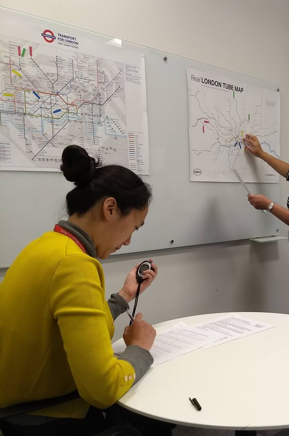
Figure 1: The London underground map (right) is a deformed map. In comparison with a relatively more faithful map (left), there is a
significant amount of information loss in the deformed map, which omits some detailed variations among different connection routes between
pairs of stations (e.g., distance and geometry). One common rationale is that the deformed map was designed for certain visualization tasks,
which likely excluded the task for estimating the walking time between a pair of stations indicated by a pair of red or blue arrows. In one
of our experiments, when asked to perform such tasks using the deformed map, some participants did rather well. Can information theory
explain this phenomenon? Can we quantitatively measure some relevant factors in this visualization process?
Abstract
Many visual representations, such as volume-rendered images and metro maps, feature a noticeable amount of information loss.
At a glance, there seem to be numerous opportunities for viewers to misinterpret the data being visualized, hence undermining
the benefits of these visual representations. In practice, there is little doubt that these visual representations are useful. The
recently-proposed information-theoretic measure for analyzing the cost-benefit ratio of visualization processes can explain
such usefulness experienced in practice, and postulate that the viewers’ knowledge can reduce the potential distortion (e.g.,
misinterpretation) due to information loss. This suggests that viewers’ knowledge can be estimated by comparing the potential
distortion without any knowledge and the actual distortion with some knowledge. In this paper, we describe several case studies
for collecting instances that can (i) support the evaluation of several candidate measures for estimating the potential distortion
distortion in visualization, and (ii) demonstrate their applicability in practical scenarios. Because the theoretical discourse
on choosing an appropriate bounded measure for estimating the potential distortion is yet conclusive, it is the real world
data about visualization further informs the selection of a bounded measure, providing practical evidence to aid a theoretical
conclusion. Meanwhile, once we can measure the potential distortion in a bounded manner, we can interpret the numerical
values characterizing the benefit of visualization more intuitively.
1. Introduction and technological advancements, but also encountered some seri-
ous contentions due to instrumental, operational, and social con-
This paper is concerned with the measurement of the benefit of ventions [Kle12]. While the development of measurement systems,
visualization and viewers’ knowledge used in visualization. The methods, and standards for visualization may take decades of re-
history of measurement science shows that the development of search, one can easily imagine their impact to visualization as a
measurements in different fields has not only stimulated scientific scientific and technological subject.
© 2021 The Author(s) with LATEX template from
Computer Graphics Forum © 2021 The Eurographics Association and John
Wiley & Sons Ltd. Published by John Wiley & Sons Ltd.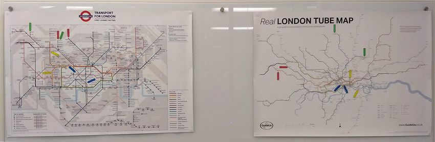
Min Chen et al. / A Bounded Measure for Estimating the Benefit of Visualization: Case Studies and Empirical Evaluation

   “Measurement ... is defined as the assignment of numerals to ob-            2. Related Work
jects or events according to rules” [Ste46]. Rules may be defined
based on physical laws (e.g., absolute zero temperature), observa-             This paper and its preceding paper (in the supplementary materials)
tional instances (e.g., the freezing and boiling points of water), or          are concerned with information-theoretic measures for quantifying
social traditions (e.g., seven days per week). Without exception,              aspects of visualization, such as benefit, knowledge, and potential
measurement development in visualization aims to discover and                  misinterpretation. The preceding paper focuses its review on previ-
define rules that will enable us to use mathematics in describing,             ous information-theoretic work in visualization. In this section, we
differentiating, and explaining phenomena in visualization, as well            focus our review on previous measurement work in visualization.
as predicting the impact of a design decision, diagnosing shortcom-            Measurement Science. There is currently no standard method
ings in visual analytics workflows, and formulating solutions for              for measuring the benefit of visualization, levels of visual abstrac-
improvement.                                                                   tion, the human knowledge used in visualization, or the potential
   In a separate and related paper (see the supplementary materi-              to misinterpret visual abstraction. While these are considered to be
als), Chen and Sbert examined a number of candidate measures for               complex undertakings, many scientists in the history of measure-
assigning numerals to the notion of potential distortion, which is             ment science would have encountered similar challenges [Kle12].
one of the three components in the information-theoretic measure                  In their book [BW08], Boslaugh and Watters describe measure-
for quantifying the cost-benefit of visualization [CG16]. They used            ment as “the process of systematically assigning numbers to objects
several “conceptual rules” to evaluate these candidates, narrowing             and their properties, to facilitate the use of mathematics in study-
them down to five candidates. In this work, we focus on the remain-            ing and describing objects and their relationships.” They empha-
ing five candidate measures and evaluate them based on empirical               size in particular measurement is not limited to physical qualities
evidence. We use two synthetic case studies and two experimental               such as height and weight, but also abstract properties such as in-
case studies to instantiate values that may be returned by the candi-          telligence and aptitude. Pedhazur and Schmelkin [PS91] assert the
dates. The main “observational rules” used in this work include:               necessity of an integrated approach for measurement development,
                                                                               involving data collection, mathematical reasoning, technology in-
a. Does the numerical ordering of observed instances match with
                                                                               novation, and device engineering. Tal [Tal20] points out that mea-
   the intuitively-expected ordering?
                                                                               surement is often not totally “real”, involves the representation of
b. Does the gap between positive and negative values indicate a
                                                                               ideal systems, and reflects conceptual, metaphysical, semantic, and
   meaningful critical point (i.e., zero benefit in our case)?
                                                                               epistemological understandings. Schlaudt [Sch20] goes one step
Although one might consider observational rules are subjective and             further, referring measurement as a cultural technique.
thus undesirable, we can appreciate their roles in the development
                                                                                  This work is particularly inspired by the historical develop-
of many measurement systems used today (e.g., number of months
                                                                               ment of temperature scales and seismic magnitude. The former at-
per year, and sign of temperature in Celsius). It would be hasty to
                                                                               tracted the attention of many well-known scientists, benefited from
dismiss such rules, especially at this early stage of measurement
                                                                               both experimental observations (e.g., by Celsius, Delisle, Fahren-
development in visualization.
                                                                               heit, Newton, etc.) and theoretical discoveries (e.g., by Boltzmann,
   In addition, we use the data collected in two visualization case            Thomson (Kelvin), etc.). The latter started not long ago as the
studies to explore the relationship between the benefit of visualiza-          Richter scale was outlined in 1935, and since then there have
tion and the viewers’ knowledge used in visualization. As shown in             been many schemes proposed relating different physical properties.
Figure 1, in one case study, we asked participants to perform tasks            Many scales in both applications are related to some logarithmic
for estimating the walking time (in minutes) between two under-                transformations one way or another.
ground stations indicated by a pair of red or blue arrows. Although
                                                                               Metrics Development in Visualization.               Behrisch et al.
the deformed London underground map was not designed to per-
                                                                               [BBK∗ 18] presented an extensive survey of quality metrics for in-
form visualization tasks, many participants performed rather well,
                                                                               formation visualization. Bertini et al. [BTK11] described a sys-
including those that had very limited experience of using the Lon-
                                                                               temic approach of using quality metrics for evaluating visualiza-
don underground. We use different candidate measures to estimate
                                                                               tion in high-dimensional data visualization focusing on scatter plots
the supposed potential distortion. When the captured data shows
                                                                               and parallel coordinates plots. A variety of quality metrics have
that the amount of actual distortion is lower than the supposed dis-
                                                                               been proposed to measure many different attributes, such as ab-
tortion, this indicate that the viewers’ knowledge has been used in
                                                                               straction quality [Tuf86, CYWR06, JC08], quality of scatter plots
the visualization process to alleviate the potential distortion. While
                                                                               [FT74, TT85, BS04, WAG05, SNLH09, TAE∗ 09, TBB∗ 10], quality
we use the experiments to collect practical instances to evaluate the
                                                                               of parallel coordinates plots [DK10], cluttering [PWR04, RLN07,
candidate measures empirically, they also demonstrate that we are
                                                                               YSZ14], aesthetics [FB09], visual saliency [JC10], and color map-
getting closer to be able to estimate the “benefit” and “potential
                                                                               ping [BSM∗ 15, MJSK15, MK15, GLS17]. In particular, Jänicke et
distortion” of practical visualization processes.
                                                                               al. [JC10] first considered a metric for estimating the amount of
   Readers are encouraged to consult the preceding paper in the                original data that is depicted by visualization and may be recon-
supplementary materials for information about the mathematical                 structed by viewers. Chen and Golan [CG16] used the abstract form
background, the formulation of some new candidate measures, and                of this idea in defining their cost-benefit ratio. While the work by
the conceptual evaluation of the candidate measures. Nevertheless,             Jänicke et al. [JC10] relied computer vision techniques to recon-
this paper is written in a self-contained manner.                              struction, this work focused on collecting and analysing empirical

                                                                                                                           © 2021 The Author(s) with LATEX template from
                                                                                   Computer Graphics Forum © 2021 The Eurographics Association and John Wiley & Sons Ltd.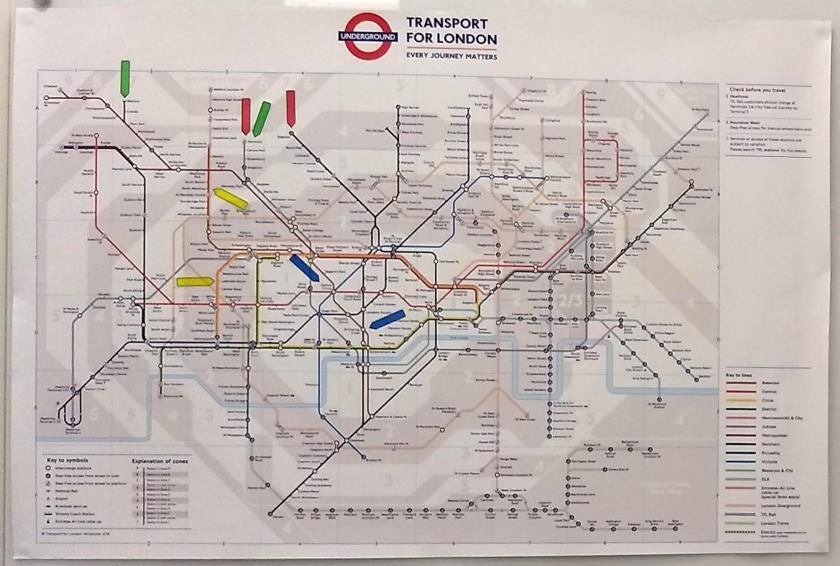
Min Chen et al. / A Bounded Measure for Estimating the Benefit of Visualization: Case Studies and Empirical Evaluation
data because human knowledge has a major role to play in infor- a1
Rules
mation reconstruction.
Measurement in Empirical Experiments. Almost all empiri-
cal studies in visualization involve measuring participants’ perfor-
mance in visualization processes. Such measured data allow us to
b1 b2 b3
assess the benefit of visualization or potential misinterpretation,
typically in terms of accuracy and response time. Many uncon-
trolled empirical studies also collect participants’ experience and
opinions qualitatively. The empirical studies related to the key com-
ponents are those on the topics of visual abstraction and human
knowledge in visualization. Isenberg [Ise13] presented a survey of c1 c2 c3
evaluation techniques on non-photorealistic and illustrative render-
ing. Isenberg et al. [INC∗ 06] reported an observational study com-
paring hand-drawn and computer-generated non-photorealistic ren-
dering. Cole et al. [CSD∗ 09] performed a study evaluating the ef-
fectiveness of line drawing in representing shape. Mandryk et al. c4 c5 c6 c7
[MML11] evaluated the emotional responses to non-photorealistic
generated images. Liu and Li [LL16] presented an eye-tracking
study examining the effectiveness and efficiency of schematic de-
sign of 30◦ and 60◦ directions in underground maps. Hong et al.
[HYC∗ 18] evaluated the usefulness of distance cartograms map “in c8 c9 c10 c11
the wild”. These studies confirmed that visualization users can deal
with significant information loss due to visual abstraction in many
situations.
Tam et al. [TKC17] reported an observational study, and discov-
ered that machine learning developers entered a huge amount of c12 c13 c14 c15
knowledge (measured in bits) into a visualization-assisted model
development process. Kijmongkolchai et al. [KARC17] reported a
study design for detecting and measuring human knowledge used
in visualization, and translated the traditional accuracy values to
information-theoretic measures. They encountered some undesir-
Figure 2: Three alphabets illustrate possible metro maps (letters)
able properties of the Kullback-Leibler divergence in their cal-
in different grid resolutions.
culations. In this work, we collect empirical data to evaluate the
mathematical solutions proposed to address the issue encountered
in [KARC17]. version is:
Benefit Alphabet Compression − Potential Distortion
= (1)
3. Overview, Notations, and Problem Statement Cost Cost
Brief Overview. Whilst hardly anyone in the visualization com- Appendix A provides more detailed explanation of this measure,
munity would support any practice intended to deceive viewers, while Appendix B explains in detail how tasks and users are con-
there have been many visualization techniques that inherently cause sidered by this measure in abstract.
distortion to the original data. The deformed London underground
Mathematical Notations. Consider a simple metro map consists
map in Figure 1 shows such an example. The distortion in this ex-
of only two stations in Figure 2. We consider three different grid
ample is largely caused by many-to-one mappings. A group of lines
resolutions, with 1 × 1 cell, 2 × 2 cells, and 4 × 4 cells respectively.
that would be shown in different lengths in a faithful map are now
The following set of rules determine whether a potential path is
shown with the same length. Another group of lines that would be
allowed or not:
shown with different geometric shapes are now shown as the same
straight line. In terms of information theory, when the faithful map • The positions of the two stations are fixed on each of the three
is transformed to the deformed, a good portion of information has grids and there is only one path between the red station and the
been lost because of these many-to-one mappings. blue station;
• As shown on the top-right of Figure 2, only horizontal, and di-
The common phrase that “the appropriateness of information
agonal path-lines are allowed;
loss depends on tasks” is not an invalid explanation. Partly by a
• When one path-line joins another, it can rotate by up to ±45◦ ;
similar conundrum in economics “what is the most appropriate res-
• All joints of path-lines can only be placed on grid points;
olution of time series for an economist”, Chen and Golan proposed
an information-theoretic cost-benefit ratio for measuring various For the first grid with 1 × 1 cell, there is only one possible path.
factors involved in visualization processes [CG16]. Its qualitative We define an alphabet A to contain this option as its only letter a1 ,
© 2021 The Author(s) with LATEX template from
Computer Graphics Forum © 2021 The Eurographics Association and John Wiley & Sons Ltd.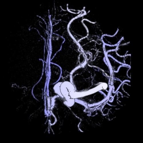
Min Chen et al. / A Bounded Measure for Estimating the Benefit of Visualization: Case Studies and Empirical Evaluation

i.e., A = {a1 }. For the second grid with 2 × 2 cells, we have an               has the PMF Qu , we have DKL (P||Qu ) ≈ 1.562 bits; and (ii) if the
alphabet B = {b1 , b2 , b3 }, consisting of three optional paths. For           original design alphabet B has the PMF Qv , we have DKL (P||Qv ) ≈
the third grid with 4 × 4 cells, there are 15 optional paths, which             0.138 bits. There is more divergence in the case (i) than case (ii).
are letters of alphabet C = {c1 , c2 , . . . , c15 }. When the resolution of    Intuitively we can guess this as P appears to be similar to Qv .
the grid increases, the alphabet of options becomes bigger quickly.
                                                                                   Recall the qualitative formula in Eq. 1. In [CG16], the benefit of
We can imagine it gradually allows the designer to create a more
                                                                                a visual analytics process is defined as:
faithful map. To ensure the calculation below is easy to follow, we
consider only the first two grids below.                                           Benefit = AC − PD = H (Zi ) − H (Zi+1 ) − DKL (Z0i ||Zi )                          (2)
   To a designer of the underground map, at the 1 × 1 resolution,               where Zi is the input alphabet to the process and Zi+1 is the output
there is only one choice regardless how much the designer would                 alphabet. Z0i is an alphabet reconstructed based on Zi+1 . Z0i has the
like to draw the path to reflect the actual geographical path of the            same set of letters as Zi but likely a different PMF.
metro line between these two stations. At the 4 × 4 resolution, the
designer has many options. Hence there is more uncertainty associ-                In terms of Eq. 2, we have Zi = B with PMF Qu or Qv , Zi+1 = A
ated with the third grid. This uncertainty can be measured by Shan-             with PMF Q, and Z0i = B0 with PMF P. We can thus calculate the
non entropy, which is defined as:                                               benefit in the two cases as:
                      n                                   n
                                                                                        Benefit of case (i) = H (B) − H (A) − DKL (B0 ||B)
       H (Z) = − ∑ pi log2 pi        where pi ∈ [0, 1], ∑ pi = 1
                    i=1                                  i=1                                                     = H (Qu ) − H (Q) − DKL (P||Qu )
where Z is an alphabet, and can be replaced with A, B, or C. To                                                  ≈ 1.585 − 0 − 1.562 = 0.023bits
calculate Shannon entropy, the alphabet Z needs to be accompanied
by a probability mass function (PMF), which is written as P(Z).                        Benefit of case (ii) = H (Qv ) − H (Q) − DKL (P||Qv )
Each letter zi ∈ Z is thus associated with a probability value pi ∈ P.
                                                                                                                 ≈ 0.569 − 0 − 0.138 = 0.431bits
Note: In this paper, to simplify the notations in different contexts,
for an information-theoretic measure, we use an alphabet Z and its              In the case (ii), because the viewers’ expectation is closer to the
PMF P interchangeably, e.g., H (P(Z)) = H (P) = H (Z). Ap-                      original PMF Qv , there is more benefit in the visualization process
pendix C provides more mathematical background about informa-                   than the case (i) though the case (ii) has less AC than case (i).
tion theory, which may be helpful to some readers.                                 However, DKL has an undesirable mathematical property. If we
   Let first consider the single-letter alphabet A and its PMF Q.               consider a third case, (iii), where the original PMF Qw is strongly
Because n = 1 and q1 = 1, we have H (A) = 0 bits. The alphabet                  in favour of b2 , such as q1 = ε, q2 = 1 − ε, q3 = ε, where 0 < ε < 1
is 100% certain, reflecting the fact that the designer has no choice.           is a small positive value. If ε = 0.001, DKL (P||Qw ) = 9.933 bits.
                                                                                If ε → 0, DKL (P||Qw ) → ∞. Since the maximum entropy (uncer-
   The alphabet B has three design options b1 , b2 , and b3 . If they           tainty) for B is only about 1.585, it is difficult to interpret that view-
have an equal chance to be selected by the designer, we have a                  ers’ divergence can be more than that maximum, not mentioning
PMF Qu with q1 = q2 = q3 = 1/3, and thus H (Qu (B)) ≈ 1.585                     the infinity.
bits. When we examine the three options in Figure 2, it is not un-
reasonable to consider a second scenario that the choice may be in              Problem Statement. When using DKL in Eq. 1 in a relative or
favour of the straight line option b1 in designing a metro map ac-              qualitative context (e.g., [CGJM19, CE19]), the unboundedness of
cording to the real geographical data. If a different PMF Qv is given           the KL-divergence does not pose an issue. However, this does be-
as q1 = 0.9, q2 = q3 = 0.05, we have H (Qv (B)) ≈ 0.569 bits. The               come an issue when the KL-divergence is used to measure PD in
second scenario features less entropy and is thus of more certainty.            an absolute and quantitative context.
   Consider that the designer is given a metro map designed using                  In the preceding paper (see the supplementary materials), Chen
alphabet B, and is asked to produce a more abstract map using al-               and Sbert showed that conceptually, it is the unboundedness is
phabet A. To the designer, it is a straightforward task, since there is         not consistent with a conceptual interpretation of KL-divergence
only one option in A. When a group of viewers are visualizing the               for measuring the inefficiency of a code (alphabet) that has a fi-
final design a1 , we could give these viewers a task to guess what              nite number of codewords (letters). They propose to find a suitable
may be the original map designed with B. If most viewers have                   bounded divergence measure to replace the DKL term. They exam-
no knowledge about the possible options b2 and b3 , and almost all              ined eight candidate measures, analysed their mathematical prop-
choose b1 as the original design, we can describe their decisions               erties with the aid of visualization, and narrowed down to five mea-
using a PMF P such that p1 = 0.998, p2 = p3 = 0.001. Since P is                 sures using multi-criteria decision analysis (MCDA) [IN13]. The
not the same as either Qu or Qv , the viewers’ decisions diverge from           upper half of Table 1 shows their conceptual evaluation based on
the actual PMF associated with B. This divergence can be measured               five criteria. In this work, we continue their MCDA process by in-
using KL-divergence:                                                            troducing criteria based on the analysis of instances obtained when
                             n                            n                     using the remaining five candidate measures in different case stud-
                                                                      pi
   DKL (P(Z)||Q(Z)) =       ∑ pi (log2 pi − log2 qi ) = ∑ pi log2 qi            ies, which correspond to criteria 6 – 9 respectively in Table 1.
                           i=1                           i=1
                                                                                   For self-containment, we give the mathematical definition of
  Using DKL , we can calculate (i) if the original design alphabet B            the five candidate measures below. In this paper, we treat them as

                                                                                                                            © 2021 The Author(s) with LATEX template from
                                                                                    Computer Graphics Forum © 2021 The Eurographics Association and John Wiley & Sons Ltd.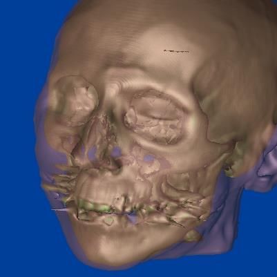
Min Chen et al. / A Bounded Measure for Estimating the Benefit of Visualization: Case Studies and Empirical Evaluation
Table 1: A summary of multi-criteria analysis. Each measure is scored against a criterion using an integer in [0, 5] with 5 being the best.
Criteria Importance 0.3DKL DJS H (P|Q) Dnew k=1 Dnew
k=2 Dncm
k=1 Dncm
k=2 Dk=2
M Dk=200
M
1. Boundedness critical 0 5 5 5 5 5 5 3 3
I 0.3DKL is eliminated but used below only for comparison. The other scores are carried forward.
2. Number of PMFs important 5 5 2 5 5 5 5 5 5
3. Entropic measures important 5 5 5 5 5 5 5 1 1
4. Curve shapes helpful 5 5 1 2 4 2 4 3 3
5. Curve shapes helpful 5 4 1 3 5 3 5 2 3
I Eliminate H (P|Q), DM 2 , D 200 based on criteria 1-5
M sum: 24 14 20 24 20 24 14 15
6. Scenario: good and bad (Figure 3) helpful − 3 − 5 4 5 4 − −
7. Scenario: A, B, C, D (Figure 4) helpful − 4 − 5 3 2 1 − −
8. Case Study 1 (Section 5.1) important − 5 − 1 5 5 5 − −
9. Case Study 2: (Section 5.2) important − 3 − 1 5 3 3 − −
I Dnew
k=2 has the highest score based on criteria 6-9 (1-9) sum: 15(39) 12(32) 17(41) 15(35) 13(37)
black-box functions, since they have already undergone the concep- which captures the non-commutative property of DKL .
tual evaluation in the preceding paper. For more detailed concep-
As DJS , Dnew
k , and D k
ncm are bounded by [0, 1], if any of them is
tual and mathematical discourse on these five candidate measures,
selected to replace DKL , Eq. 2 can be rewritten as
please consult the preceding paper in the supplementary materials.
Benefit = H (Zi ) − H (Zi+1 ) − Hmax (Zi )D(Z0i ||Zi ) (6)
The first candidate measure is Jensen-Shannon divergence
[Lin91]. The conceptual evaluation yield a promising score of 24 where Hmax denotes maximum entropy, while D is a placeholder
in Table 1. It is defined as: for DJS , Dnew
k , or D k .
ncm
1
DJS (P||Q) = DKL (P||M) + DKL (Q||M) = DJS (Q||P)
2
(3) 4. Synthetic Case Studies
1 n
2pi 2qi
= ∑ pi log2 + qi log2
2 i=1 pi + qi pi + qi The work in this section and the next section is inspired by the
historical development of temperature scales, in which many pio-
where P and Q are two PMFs associated with the same alphabet Z neering scientists collected observational data to help reason about
and M is the average distribution of P and Q. Each letter zi ∈ Z is the candidate scales. We first consider two synthetic case studies,
associated with a probability value pi ∈ P and another qi ∈ Q. With which allow us to define idealized situations, from which collected
the base 2 logarithm as in Eq. 3, DJS (P||Q) is bounded by 0 and 1. data do not contain any noise. We use these case studies to see if
The second and third candidate measures are two instances of a the values returned by different divergence measures make sense.
new measure Dnewk proposed by Chen and Sbert in the preceding In many ways, this is similar to testing a piece of software using
work. The two instances are Dnewk (k = 1) and D k (k = 2). They pre-defined test cases. Nevertheless, these test cases feature more
new
received scores of 20 and 24 respectively in the conceptual evalua- complex alphabets than those considered by the conceptual evalu-
tion. Dnew
k is defined as follows: ation reported in the preceding paper. In our analysis, we followed
the best-worst method of MCDA [Rez15]. Our main “observational
1 n rules” are:
Dnew
k
(pi + qi ) log2 |pi − qi |k + 1
(P||Q) = ∑ (4)
2 i=1
a. Does the numerical ordering of observed instances match with
where k > 0. Because 0 ≤ |pi − qi ≤ 1, we have|k the intuitively-expected ordering?
b. Does the gap between positive and negative values indicate a
1 n 1 n
∑ (pi +qi ) log2 (0+1) ≤ Dnew
k
(P||Q) ≤ ∑ (pi +qi ) log2 (1+1) meaningful critical point (i.e., zero benefit in our case)?
2 i=1 2 i=1
Criterion 6. Let Z be an alphabet with two letters, good and
Since log2 1 = 0, log2 2 = 1, ∑ pi = 1, ∑ qi = 1, Dnew
k (P||Q) is thus
bad, for describing a scenario (e.g., an object or an event), which
bounded by 0 and 1. has the probability of good is p1 = 0.8, and that of bad is p2 = 0.2.
In other words, P = {0.8, 0.2}. Imagine that a biased process (e.g.,
The fourth and five candidate measures are two instances of a
a distorted visualization, an incorrect algorithm, or a misleading
non-commutative version of Dnew k . It is denoted as D k , and the
ncm communication) conveys the information about the scenario always
two instances are Dncm
k (k = 1) and D k (k = 2). They also received
ncm bad, i.e., a PMF Rbiased = {0, 1}. Users at the receiving end of the
scores of 20 and 24 respectively in the conceptual evaluation. Dncm
k
process may have different knowledge about the actual scenario,
is defined as follows:
and they will make a decision after receiving the output of the pro-
n
cess. For example, there are five users and we have obtained the
Dncm
k
|pi − qi |k + 1
(P||Q) = ∑ pi log2 (5)
i=1 probability of their decisions as follows:
© 2021 The Author(s) with LATEX template from
Computer Graphics Forum © 2021 The Eurographics Association and John Wiley & Sons Ltd.
Min Chen et al. / A Bounded Measure for Estimating the Benefit of Visualization: Case Studies and Empirical Evaluation
1.0 ground truth distribution P
Divergence Contributions to the divergence from different letters misleading Rbiased
0.9 reconstructed Q
Good Bad
0.8
LD: a little
0.7 doubt
0.6 FD: a fair
amount
0.5 of doubt
0.4
RG: random
0.3 guess
0.2
UC: under-
0.1 correction
0.0
LD DF RG UC OC LD DF RG UC OC LD DF RG UC OC LD DF RG UC OC LD DF RG UC OC OC: over-
correction
DJS Dncm (k=1) Dncm (k=2) Dnew (k=1) Dnew (k=2)
Figure 3: An example scenario with two states good and bad has a ground truth PMF P = {0.8, 0.2}. From the output of a biased process
that always informs users that the situation is bad. Five users, LD, DF, RG, UC, and OC, have different knowledge, and thus different
divergence. The five candidate measures return different values of divergence. We would like to see which set of values are more intuitive. The
illustration on the right shows two transformations of the alphabets and their PMFs, one by the misleading communication and the other by
the reconstruction.
0.4 ground truth distribution P
Divergence Contributions to the divergence from different letters correct/biased R
A B C D reconstructed Q
CG: correct
0.3 pr. & guess
CU: correct
pr. & useful
knowledge
0.2 CB: correct
pr. & biased
reasoning
BG: biased
0.1 pr. & guess
BS: biased
pr. & small
correction
0.0
BM: biased
CG CU CB BG BS BM CG CU CB BG BS BM CG CU CB BG BS BM CG CU CB BG BS BM CG CU CB BG BS BM pr. & major
DJS Dncm (k=1) Dncm (k=2) Dnew (k=1) Dnew (k=2) correction
Figure 4: An example scenario with four data values: A, B, C, and D. Two processes (one correct and one biased) aggregated them to two
values AB and CD. Users CG, CU, CB attempt to reconstruct [A, B, C, D] from the output [AB, CD] of the correct process, while BG, BS,
and BM attempt to do so with the output from the biased processes. The bar chart shows divergence values of the six users computed using
the five candidate measures. The illustration on the right shows two transformations of the alphabets and their PMFs, one by the correct or
biased process (pr.) and the other by the reconstruction.
• LD — The user has a little doubt about the output of the process, slightly more divergence than UC (0.014 vs. 0.010). DJS returns
and decides bad 90% of the time, and good 10% of the time, i.e., relatively low values than other measures. For UC and OC, DJS ,
with PMF Q = {0.1, 0.9}. Dncm
k=1 , and D k=2 return small values (< 0.02), which are a bit dif-
new
• FD — The user has a fair amount of doubt, with Q = {0.3, 0.7}. ficult to estimate.
• RG — The user makes a random guess, with Q = {0.5, 0.5}.
Dncm
k=1 and D k=2 show strong asymmetric patterns between good
ncm
• UC — The user has adequate knowledge about P, but under-
and bad, reflecting the probability values in Q. In other words,
compensate it slightly, with Q = {0.7, 0.3}.
the more decisions on good, the more good-related divergence.
• OC — The user has adequate knowledge about P, but over-
This asymmetric pattern is not in anyway incorrect, as the KL-
compensate it slightly, with Q = {0.9, 0.1}.
divergence is also non-commutative and would also produce much
stronger asymmetric patterns. An argument for supporting commu-
We can use different candidate measures to compute the diver-
tative measures would point out that the higher probability of good
gence between P and Q. Figure 3 shows different divergence val-
in P should also influence the balance between the good-related
ues returned by these measures, while the transformations from P to
divergence.
Rbiased and then to Q are illustrated on the right margin of the figure.
Each value is decomposed into two parts, one for good and one for We decide to score DJS 3 because of its lower valuation and its
bad. All these measures can order these five users reasonably well. non-equal comparison of OU and OC. We score Dncm k=1 and D k=1
new
The users UC (under-compensate) and OC (over-compensate) have 5; and Dncm and Dnew 4 as the values returned by Dncm
k=2 k=2 k=1 and D k=1
new
the same values with Dnewk and D k , while D considers OC has
ncm JS are slightly more intuitive.
© 2021 The Author(s) with LATEX template from
Computer Graphics Forum © 2021 The Eurographics Association and John Wiley & Sons Ltd.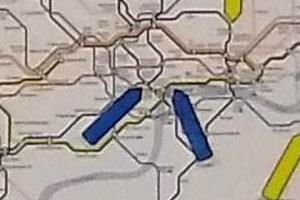
Min Chen et al. / A Bounded Measure for Estimating the Benefit of Visualization: Case Studies and Empirical Evaluation

Criterion 7. We now consider a slightly more complicated sce-                             Question 5: The image on the right depicts a computed
                                                                                          tomography dataset (arteries) that was rendered using a
nario with four pieces of data, A, B, C, and D, which can be de-                          maximum intensity projection (MIP) algorithm. Consider
                                                                                          the section of the image inside the red circle (also in the
                                                                                          inset of a zoomed-in view). Which of the following
fined as an alphabet Z with four letters. The ground truth PMF is                         illustrations would be the closest to the real surface of
P = {0.1, 0.4, 0.2, 0.3}. Consider two processes that combine these                       this part of the artery?

into two classes AB and CD. These typify clustering algorithms,
downsampling processes, discretization in visual mapping, and so                          A                                B
                                                                                                    Curved,                             Curved,
on. One process is considered to be correct, which has a PMF for                                 rather smooth                 with wrinkles and bumps

AB and CD as Rcorrect = {0.5, 0.5}, and another biased process
with Rbiased = {0, 1}. Let CG, CU, and CH be three users at the                           C                                D
receiving end of the correct process, and BG, BS, and BM be three                                     Flat,
                                                                                                 rather smooth
                                                                                                                                         Flat,
                                                                                                                               with wrinkles and bumps
other users at the receiving end of the biased process. The users
with different knowledge exhibit different abilities to reconstruct                      Figure 5: A volume dataset was rendered using the MIP method. A
the original scenario featuring A, B, C, D from aggregated infor-                        question about a “flat area” in the image can be used to tease out
                                                                                                                                               Image by Min Chen, 2008
mation about AB and CD. Similar to the good-bad scenario, such                           a viewer’s knowledge that is useful in a visualization process.
abilities can be captured by a PMF Q. For example, we have:
•   CG makes random guess, Q = {0.25, 0.25, 0.25, 0.25}.
                                                                                         compression. Some major algorithmic functions in volume visual-
•   CU has useful knowledge, Q = {0.1, 0.4, 0.1, 0.4}.
                                                                                         ization, e.g., iso-surfacing, transfer function, and rendering integral,
•   CB is highly biased, Q = {0.4, 0.1, 0.4, 0.1}.
                                                                                         all facilitate alphabet compression, hence information loss.
•   BG makes guess based on Rbiased , Q = {0.0, 0.0, 0.5, 0.5}.
•   BS makes a small adjustment, Q = {0.1, 0.1, 0.4, 0.4}.                                  In terms of rendering integral, maximum intensity projection
•   BM makes a major adjustment, Q = {0.2, 0.2, 0.3, 0.3}.                               (MIP) incurs a huge amount of information loss in comparison with
Figure 4 compares the divergence values returned by the candi-                           the commonly-used emission-and-absorption integral [MC10]. As
date measures for these six users, while the transformations from                        shown in Figure 5, the surface of arteries are depicted more or less
P to Rcorrect or Rbiased , and then to Q are illustrated on the right.                   in the same color. The accompanying question intends to tease out
We can observe that Dncm   k  and Dnew
                                     k=2 return values < 0.1, which                      two pieces of knowledge, “curved surface” and “with wrinkles and
seem to be less intuitive. Meanwhile DJS shows a large portion                           bumps”. Among the ten surveyees, one selected the correct answer
of divergence from the AB category, while Dncm   k=1 and D k=2 show                      B, eight selected the relatively plausible answer A, and one selected
                                                           ncm
more divergence in the BC category. In particular, for user BG,                          the doubtful answer D.
Dncm
  k=1 and D k=2 do not show any divergence in relation to A and B,
             ncm                                                                            Let alphabet Z = {A, B, C, D} contain the four optional answers.
though BG clearly has reasoned A and B rather incorrectly. Dnew   k=1
                                                                                         One may assume a ground truth PMF Q = {0.1, 0.878, 0.002, 0.02}
and Dnew show a relatively balanced account of divergence associ-
      k=2
                                                                                         since there might still be a small probability for a section of
ated with A, B, C, and D. On balance, we give scores 5, 4, 3, 2, 1                       artery to be flat or smooth. The rendered image depicts a mis-
to Dnew
     k=1 , D , D k=2 , D k=1 , and D k=2 respectively.
            JS   new      ncm        ncm                                                 leading impression, implying that answer C is correct or a false
                                                                                         PMF F = {0, 0, 1, 0}. The amount of alphabet compression is thus
5. Experimental Case Studies                                                             H (Q) − H (F) = 0.225.
To complement the synthetic case studies in Section 4, we con-                              When a surveyee gives an answer to the question, it can also be
ducted two surveys to collect some realistic examples that feature                       considered as a PMF P. With PMF Q = {0.1, 0.878, 0.002, 0.02},
the use of knowledge in visualization. In addition to providing in-                      different answers thus lead to different values of divergence as fol-
stances of criteria 8 and 9 for selecting a bounded measure, the                         lows:
surveys were also designed to demonstrate that one could use a few                       Divergence for:                                          DJS    Dnew
                                                                                                                                                          k=1     Dnew
                                                                                                                                                                   k=2    Dncm
                                                                                                                                                                           k=1    Dncm
                                                                                                                                                                                   k=2
simple questions to estimate the cost-benefit of visualization in re-
lation to individual users.                                                              A (Pa = {1, 0, 0, 0}, Q):                              0.758    0.9087   0.833   0.926   0.856
                                                                                         B (Pb = {0, 1, 0, 0}, Q):                              0.064    0.1631   0.021   0.166   0.021
                                                                                         C (Pc = {0, 0, 1, 0}, Q):                              0.990    0.9066   0.985   0.999   0.997
5.1. Volume Visualization (Criterion 8)                                                  D (Pd = {0, 0, 0, 1}, Q):                              0.929    0.9086   0.858   0.986   0.971
This survey, which involved ten surveyees, was designed to collect
some real-world data that reflects the use of knowledge in view-                            Without any knowledge, a surveyee would select answer C, lead-
ing volume visualization images. The full set of questions were                          ing to the highest value of divergence in terms of any of the three
presented to surveyees in the form of slides, which are included                         measures. Based PMF Q, we expect to have divergence values in
in the supplementary materials. The full set of survey results is                        the order of C > D > A  B. DJS , Dnew  k=2 , D k=1 , and D k=2 have
                                                                                                                                        ncm         ncm
given in Appendix C. The featured volume datasets were from                              produced values in that order, while Dnew
                                                                                                                                k=1 indicates an order of A

“The Volume Library” [Roe19], and visualization images were ei-                          > D > C  B. This order cannot be interpreted easily, indicating
ther rendered by the authors or from one of the four publications                        a weakness of Dnew
                                                                                                          k=1 .

[NSW02, CSC06, WQ07, Jun19].
                                                                                            Together with the alphabet compression H (Q) − H (F) =
   The transformation from a volumetric dataset to a volume-                             0.225 and the Hmax of 2 bits, we can also calculate the informative
rendered image typically features a noticeable amount of alphabet                        benefit using Eq. 6. For surveyees with different answers, the lossy

© 2021 The Author(s) with LATEX template from
Computer Graphics Forum © 2021 The Eurographics Association and John Wiley & Sons Ltd.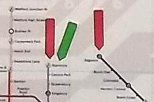
Min Chen et al. / A Bounded Measure for Estimating the Benefit of Visualization: Case Studies and Empirical Evaluation
Benefit for: DJS Dnew
k=1 Dnew
k=2 Dncm
k=1 Dncm
k=2
Meanwhile, the voxels for soft tissue and muscle are not depicted at
A (Pa = {1, 0, 0, 0}, Q): −0.889 −1.190 −1.038 −1.224 −1.084 all, which can also been regarded as using a hollow visual channel.
B (Pb = {0, 1, 0, 0}, Q): 0.500 0.302 0.586 0.296 0.585 The visual representation has been widely used, and the viewers
C (Pc = {0, 0, 1, 0}, Q): −1.351 −1.185 −1.097 −1.369 −1.366 are expected to use their knowledge to infer the 3D relationships
D (Pd = {0, 0, 0, 1}, Q): −1.230 −1.189 −1.088 −1.343 −1.314 between the two iso-surfaces as well as the missing information
Question 3: The image on the right depicts a computed
about soft tissue and muscle. The question that accompanies the
tomography dataset (head) that was rendered using a
ray casting algorithm. Consider the section of the image
figure is for estimating such knowledge.
inside the orange circle. Which of the following
illustrations would be the closest to the real cross
section of this part of the facial structure? Although the survey offers only four options, it could in fact of-
fer many other configurations as optional answers. Let us consider
four color-coded segments similar to the configurations in answers
A B
C and D. Each segment could be one of four types: bone, skin, soft
tissue and muscle, or background. There are a total of 44 = 256 con-
figurations. If one had to consider the variation of segment thick-
C D ness, there would be many more options. Because it would not be
appropriate to ask a surveyee to select an answer from 256 options,
a typical assumption is that the selected four options are represen-
background bone skin soft tissue and muscle
tative. In other words, considering that the 256 options are letters
Figure 6: Two iso-surfaces of a volume dataset wereImage by Min Chen, 1999
rendered us- of an alphabet, any unselected letter has a probability similar to one
ing the ray casting method. A question about the tissue configura- of the four selected options.
tion in the orange circle can tease out a viewer’s knowledge about For example, we can estimate a ground truth PMF Q such that
the translucent depiction and the missing information. among the 256 letters,
• Answer A and four other letters have a probability 0.01,
depiction of the surface of arteries brought about different amounts
• Answer B and 64 other letters have a probability 0.0002,
of benefit:
• Answer C and 184 other letters have a probability 0.0001,
All five sets of values indicate that only those surveyees who • Answer D has a probability 0.9185.
gave answer C would benefit from such lossy depiction produced
by MIP, signifying the importance of user knowledge in visualiza- We have the entropy of this alphabet H (Q) = 0.85. Similar to the
tion. However, the values returned for A, C, and D by Dnew k=1 are previous example, we can estimate the values of divergence as:
almost indistinguishable and in an undesirable order. Divergence for: DJS Dnew
k=1 Dnew
k=2 Dncm
k=1 Dncm
k=2
One may also consider the scenarios where flat or smooth sur- .... .... ....
A: P = {1, 4 , 0, 64 , 0, 184 , 0} 0.960 0.933 0.903 0.993 0.986
faces are more probable. For example, if the ground truth PMF were .... .... ....
B: P = {0, 4 , 1, 64 , 0, 184 , 0} 0.999 0.932 0.905 1.000 1.000
Q0 = {0.30, 0.57, 0.03, 0.10} and H (Q0 ) = 1.467, the amounts of .... .... ....
C: P = {0, 4 , 0, 64 , 1, 184 , 0} 0.999 0.932 0.905 1.000 1.000
benefit would become: .... .... ....
D: P = {0, 4 , 0, 64 , 0, 184 , 1} 0.042 0.109 0.009 0.113 0.010
Benefit for: DJS Dnew k=1 D k=2
new Dncm
k=1 Dncm
k=2
A (Pa = {1, 0, 0, 0}, Q0 ): 0.480 0.086 0.487 −0.064 0.317 where ....
n denotes n zeros. DJS , Dnew , Dncm and Dncm returned
k=2 k=1 k=2
B (Pb = {0, 1, 0, 0}, Q0 ): 0.951 0.529 1.044 0.435 0.978 values indicating the same order of divergence, i.e., C ∼ B > A
C (Pc = {0, 0, 1, 0}, Q0 ): −0.337 −0.038 0.212 −0.489 −0.446 D, which is consistent with PMF Q0 . Only Dnew k=1 returns an order
D (Pd = {0, 0, 0, 1}, Q0 ): −0.049 −0.037 0.257 −0.385 −0.245 A > B ∼ C
D. This reinforces the observation by the previous
example (i.e., Figure 5) about the characteristics of ordering of the
Because the ground truth PMF Q0 would be less certain, the knowl- five measures.
edge of “curved surface” and “with wrinkles and bumps” would
For both examples (Figs. 5 and 6), because both DJS , Dnew k=2 ,
become more useful. Further, because the probability of flat and
Dncm
k=1 and Dncm have consistently returned sensible values, we give
k=2
smooth surfaces would have increased, an answer C would not be
a score of 5 to each of them in Table 1. Dnew
k=1 appears to be often
as bad as when it is with the original PMF Q. Among the five mea-
incompatible with other measures in terms of ordering, we score
sures, DJS , Dnew
k=2 , D k=1 , and D k=2 returned values indicating the
ncm ncm Dnew
k=1 1.
same order of benefit, i.e., B > A > D > C, which is consistent
with PMF Q0 . Only Dnewk=1 orders C and D differently.
We can also observe that these measures occupy different ranges 5.2. London Underground Map (Criterion 9)
of real values. Dnew
k=2 appears to be more generous in valuing the
This survey was designed to collect some real-world data that re-
benefit of visualization, while Dncm
k=1 is less generous. We will ex-
flects the use of knowledge in viewing different London under-
amine this phenomenon with a more compelling example in Sec-
ground maps. It involved sixteen surveyees, twelve at King’s Col-
tion 5.2.
lege London (KCL) and four at University of Oxford. Surveyees
Figure 6 shows another volume-rendered image used in the sur- were interviewed individually in a setup as shown in Figure 7.
vey. Two iso-surfaces of a head dataset are depicted with translu- Each surveyee was asked to answer 12 questions using either a
cent occlusion, which is a type of visual multiplexing [CWB∗ 14]. geographically-faithful map or a deformed map, followed by two
© 2021 The Author(s) with LATEX template from
Computer Graphics Forum © 2021 The Eurographics Association and John Wiley & Sons Ltd.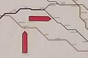
Min Chen et al. / A Bounded Measure for Estimating the Benefit of Visualization: Case Studies and Empirical Evaluation
Figure 7: A survey for collecting data that reflects the use of some knowledge in viewing two types of London underground maps.
further questions about their familiarity of a metro system and Lon- approximate the PMF as Q = {qi | 1 ≤ i ≤ 256}, where
don. A £5 Amazon voucher was offered to each surveyee as an ap-
preciation of their effort and time. The survey sheets and the full
0.01/236 if 1 ≤ i ≤ ξ − 8 (wild guess)
0.026 if ξ − 7 ≤ i ≤ ξ − 3 (close)
set of survey results are given in Appendix D.
qi = 0.12 if ξ − 2 ≤ i ≤ ξ + 2 (spot on)
0.026 if ξ + 3 ≤ i ≤ ξ + 12 (close)
Harry Beck first introduced geographically-deformed design of
0.01/236 if ξ + 13 ≤ i ≤ 256 (wild guess)
the London underground maps in 1931. Today almost all metro
maps around the world adopt this design concept. Information- Using the same way in the previous case study, we can estimate the
theoretically, the transformation of a geographically-faithful map divergence and the benefit of visualization for an answer in each
to such a geographically-deformed map causes a significant loss of range. Recall our observation of the phenomenon in Section 5.1
information. Naturally, this affects some tasks more than others. that the measurements by DJS, Dnew k=1 , D k=2 , D k=1 and D k=2 oc-
new ncm ncm
cupy different ranges of values, with Dnew k=2 be the most generous
in measuring the benefit of visualization. With the entropy of the
For example, the distances between stations on a deformed map alphabet as H (Q) ≈ 3.6 bits and the maximum entropy being 8
are not as useful as in a faithful map. The first four questions in the bits, the benefit values obtained for this example exhibit a similar
survey asked surveyees to estimate how long it would take to walk but more compelling pattern:
(i) from Charing Cross to Oxford Circus, (ii) from Temple and Le-
icester Square, (iii) from Stanmore to Edgware, and (iv) from South Benefit for: DJS Dnew
k=1 Dnew
k=2 Dncm
k=1 Dncm
k=2
Rulslip to South Harrow. On the deformed map, the distances be- spot on −1.765 −0.418 0.287 −3.252 −2.585
tween the four pairs of the stations are all about 50mm. On the close −3.266 −0.439 0.033 −3.815 −3.666
faithful map, the distances are (i) 21mm, (ii) 14mm, (iii) 31mm, wild guess −3.963 −0.416 −0.017 −3.966 −3.965
and (iv) 53mm respectively. According to the Google map, the es-
timated walk distance and time are (i) 0.9 miles, 20 minutes; (ii) 0.8 Only Dnew
k=2 has returned positive benefit values for spot on and
miles, 17 minutes; (iii) 1.6 miles, 32 minutes; and (iv) 2.2 miles, 45 close answers. Since it is not intuitive to say that those surveyees
minutes respectively. who gave good answers benefited from visualization negatively,
clearly only the measurements returned by Dnew k=2 are intuitive. In
addition, the ordering resulting from Dnew k=1 is again inconsistent
The average range of the estimations about the walk time by the with others.
12 surveyees at KCL are: (i) 19.25 [8, 30], (ii) 19.67 [5, 30], (iii)
For instance, surveyee P9, who has lived in a city with a metro
46.25 [10, 240], and (iv) 59.17 [20, 120] minutes. The estimations
system for a period of 1-5 years and lived in London for several
by the four surveyees at Oxford are: (i) 16.25 [15, 20], (ii) 10 [5,
months, made similarly good estimations about the walking time
15], (iii) 37.25 [25, 60], and (iv) 33.75 [20, 60] minutes. The values
with both types of underground maps. With one spot on answer
correlate better to the Google estimations than what would be im-
and one close answer under each condition, the estimated benefit
plied by the similar distances on the deformed map. Clearly some
on average is 0.160 bits if one uses Dnew k=2 and is negative if one
surveyees were using some knowledge to make better inference.
uses any of the other four measures. Meanwhile, surveyee P3, who
has lived in a city with a metro system for two months, provided all
four answers in the wild guess category, leading to negative benefit
Let Z be an alphabet of integers between 1 and 256. The range
values by all five measures.
is chosen partly to cover the range of the answers in the survey, and
partly to round up the maximum entropy Z to 8 bits. For each pair Similarly, among the first set of four questions in the survey,
of stations, we can define a PMF using a skew normal distribution Questions 1 and 2 are about stations near KCL, and Questions 3
peaked at the Google estimation ξ . As an illustration, we coarsely and 4 are about stations more than 10 miles away from KCL. The
© 2021 The Author(s) with LATEX template from
Computer Graphics Forum © 2021 The Eurographics Association and John Wiley & Sons Ltd.
Min Chen et al. / A Bounded Measure for Estimating the Benefit of Visualization: Case Studies and Empirical Evaluation

local knowledge of the surveyees from KCL clearly helped their                    This cost-benefit measure was developed in the field of visual-
answers. Among the answers given by the twelve surveyees from                  ization, for optimizing visualization processes and visual analytics
KCL,                                                                           workflows. Its broad interpretation may include data intelligence
                                                                               workflows in other contexts [Che20]. The measure has now been
• For Question 1, four spot on, five close, and three wild guess —
                                                                               improved by using visual analysis and with the survey data col-
  the average benefit is −2.940 with DJS or 0.105 with Dnewk=2 .
                                                                               lected in the context of visualization applications.
• For Question 2, two spot on, nine close, and one wild guess —
  the average benefit is −3.074 with DJS or 0.071 with Dnewk=2 .                  The history of measurement science [Kle12] informs us that pro-
• For Question 3, three close, and nine wild guess — the average               posals for metrics, measures, and scales will continue to emerge in
  benefit is −3.789 with DJS or −0.005 with Dnew k=2 .                         visualization, typically following the arrival of new theoretical un-
• For Question 4, two spot on, one close, and nine wild guess —                derstanding, new observational data, new measurement technology,
  the average benefit is with −3.539 DJS or 0.038 with Dnewk=2 .               and so on. As measurement is one of the driving forces in science
                                                                               and technology. We shall welcome such new measurement devel-
   The average benefit values returned by Dnewk=1 , D k=1 , and D k=2
                                                     ncm         ncm           opment in visualization.
are all negative for these four questions. Hence, unless Dnew  k=2 is

used, all other measures would semantically imply that both types                 The work presented in this paper and the preceding paper does
of the London underground maps would have negative benefit. We                 not indicate a closed chapter, but an early effort to be improved
therefore give Dnew
                 k=2 a 5 score and D , D k=1 , and D k=2 a 3 score
                                     JS    ncm         ncm                     frequently in the future. For example, future work may discover
each in Table 1. We score Dnewk=1 1 as it also exhibits an ordering            measures that have better mathematical properties than Dnewk   and
issue.                                                                         DJS , or future experimental observation may evidence that DJS of-
                                                                               fer more intuitive explanations than Dnew
                                                                                                                      k  in other case studies. In
   When we consider answering each of Questions 1∼4 as perform-                particular, we would like to continue our theoretical investigation
ing a visualization task, we can estimate the cost-benefit ratio of            into the mathematical properties of Dnew
                                                                                                                     k .
each process. As the survey also collected the time used by each
surveyee in answering each question, the cost in Eq. 1 can be ap-                 “Measurement is not an end but a means in the process of de-
proximated with the mean response time. For Questions 1∼4, the                 scription, differentiation, explanation, prediction, diagnosis, deci-
mean response times by the surveyees at KCL are 9.27, 9.48, 14.65,             sion making, and the like” [PS91]. Having a bounded cost-benefit
and 11.40 seconds respectively. Using the benefit values based on              measure offers many new opportunities of developing tools for aid-
Dnew
  k=2 , the cost-benefit ratios are thus 0.0113, 0.0075, -0.0003, and          ing the measurement and using such tools in practical applications,
0.0033 bits/second respectively. While these values indicate the               especially in visualization and visual analytics.
benefits of the local knowledge used in answering Questions 1 and
2, they also indicate that when the local knowledge is absent in the
case of Questions 3 and 4, the deformed map (i.e., Question 3) is              References
less cost-beneficial.                                                          [BBK∗ 18] B EHRISCH M., B LUMENSCHEIN M., K IM N. W., S HAO L.,
                                                                                 E L -A SSADY M., F UCHS J., S EEBACHER D., D IEHL A., B RANDES U.,
                                                                                 P FISTER H., S CHRECK T., W EISKOPF D., K EIM D. A.: Quality metrics
6. Conclusions                                                                   for information visualization. Computer Graphics Forum 37, 3 (2018),
                                                                                 625–662. 2
This paper is a follow-on paper that continues an investigation                [BS04] B ERTINI E., S ANTUCCI G.: Quality metrics for 2D scatterplot
into the need to improve the mathematical formulation of an                      graphics: Automatically reducing visual clutter. In Smart Graphics, Butz
information-theoretic measure for analyzing the cost-benefit of vi-              A., Krüger A., Olivier P., (Eds.), vol. 3031 of Lecture Notes in Computer
sualization as well as other processes in a data intelligence work-              Science. Springer Berlin Heidelberg, Berlin, Heidelberg, 2004, pp. 77–
flow [CG16]. The concern about the original measure is its un-                   89. 2
bounded term based on the KL-divergence. The preceding paper                   [BSM∗ 15] B ERNARD J., S TEIGER M., M ITTELSTÄDT S., T HUM S.,
(in the supplementary materials) studied eight candidate measures                K EIM D. A., KOHLHAMMER J.: A survey and task-based quality as-
                                                                                 sessment of static 2d color maps. In Proc. of SPIE 9397, Visualization
and use conceptual evaluation to narrow the options down to five,                and Data Analysis (2015). 2
providing important evidence to the multi-criteria analysis of thees
                                                                               [BTK11] B ERTINI E., TATU A., K EIM D.: Quality metrics in high-
candidate measures.
                                                                                 dimensional data visualization: An overview and systematization. IEEE
   From Table 1, we can observe the process of narrowing down                    Trans. Visualization & Computer Graphics 17, 12 (2011), 2203–2212. 2
from eight candidate measures to five measures, and then to one.               [BW08] B OSLAUGH S., WATTERS P. A.: Statistics in a Nutshell: A
Taking the importance of the criteria into account, we consider that             Desktop Quick Reference Paperback. O’Reilly, 2008. 2
candidate Dnew
             k (k = 2) is ahead of D , critically because D often
                                     JS                      JS                [CE19] C HEN M., E BERT D. S.: An ontological framework for sup-
yields negative benefit values even when the benefit of visualization            porting the design and evaluation of visual analytics systems. Computer
                                                                                 Graphics Forum 38, 3 (2019), 131–144. 4, 13, 16
is clearly there. We therefore propose to revise the original cost-
benefit ratio in [CG16] to the following:                                      [CE20] C HEN M., E DWARDS D. J.: ‘isms’ in visualization. In Founda-
                                                                                 tions of Data Visualization, Chen M., Hauser H., Rheingans P., Scheuer-
   Benefit Alphabet Compression − Potential Distortion                           mann G., (Eds.). Springer, 2020. 13
          =
    Cost                        Cost                                           [CG16] C HEN M., G OLAN A.: What may visualization processes opti-
                                                                    (7)
            H (Zi ) − H (Zi+1 ) − Hmax (Zi )Dnew
                                             2 (Z0 ||Z )
                                                 i    i                          mize? IEEE Trans. Visualization & Computer Graphics 22, 12 (2016),
          =                                                                      2619–2632. 2, 3, 4, 10, 13, 14, 15
                                Cost

                                                                                                                           © 2021 The Author(s) with LATEX template from
                                                                                   Computer Graphics Forum © 2021 The Eurographics Association and John Wiley & Sons Ltd.
Min Chen et al. / A Bounded Measure for Estimating the Benefit of Visualization: Case Studies and Empirical Evaluation
[CGJM19] C HEN M., G AITHER K., J OHN N. W., M C C ANN B.: Cost- [KL51] K ULLBACK S., L EIBLER R. A.: On information and sufficiency.
benefit analysis of visualization in virtual environments. IEEE Trans. Annals of Mathematical Statistics 22, 1 (1951), 79–86. 15
Visualization & Computer Graphics 25, 1 (2019), 32–42. 4 [Kle12] K LEIN H. A.: The Science of Measurement: A Historical Survey.
[Che18] C HEN M.: The value of interaction in data intelligence. Dover Publications, 2012. 1, 2, 10
arXiv:1812.06051, 2018. 15 [KS14] K INDLMANN G., S CHEIDEGGER C.: An algebraic process for
[Che20] C HEN M.: Cost-benefit analysis of data intelligence – its broader visualization design. IEEE Transactions on Visualization and Computer
interpretations. In Advances in Info-Metrics: Information and Informa- Graphics 20, 12 (2014), 2181–2190. 14
tion Processing across Disciplines, Chen M., Dunn J. M., Golan A., Ul- [Lin91] L IN J.: Divergence measures based on the shannon entropy.
lah A., (Eds.). Oxford University Press, 2020. 10 IEEE Transactions on Information Theory 37 (1991), 145–151. 5
[CSC06] C ORREA C., S ILVER D., C HEN M.: Feature aligned volume [LL16] L IU Z., L I Z.: Impact of schematic designs on the cognition
manipulation for illustration and visualization. IEEE Trans. Visualization of underground tube maps. ISPRS - International Archives of the Pho-
& Computer Graphics 12, 5 (2006), 1069–1076. 7 togrammetry, Remote Sensing and Spatial Information Sciences (2016),
[CSD∗ 09] C OLE F., S ANIK K., D E C ARLO D., F INKELSTEIN A., 421–423. 3
F UNKHOUSER T., RUSINKIEWICZ S., S INGH M.: How well do line [MC10] M AX N., C HEN M.: Local and global illumination in the vol-
drawings depict shape? In ACM SIGGRAPH 2009 Papers (2009), SIG- ume rendering integral. In Scientific Visualization: Advanced Concepts,
GRAPH ’09. 3 Hagen H., (Ed.). Schloss Dagstuhl, Wadern, Germany, 2010. 7
[CTBA∗ 11] C HEN M., T REFETHEN A., BANARES -A LCANTARA R., [MJSK15] M ITTELSTÄDT S., J ÄCKLE D., S TOFFEL F., K EIM D. A.:
J IROTKA M., C OECKE B., E RTL T., S CHMIDT A.: From data analysis ColorCAT : Guided design of colormaps for combined analysis tasks.
and visualization to causality discovery. IEEE Computer 44, 11 (2011), In Eurographics Conference on Visualization (EuroVis) : Short Papers
84–87. 15 (2015), Bertini E., (Ed.), pp. 115–119. 2
[CWB∗ 14] C HEN M., WALTON S., B ERGER K., T HIYAGALINGAM J., [MK15] M ITTELSTÄDT S., K EIM D. A.: Efficient contrast effect com-
D UFFY B., FANG H., H OLLOWAY C., T REFETHEN A. E.: Visual mul- pensation with personalized perception models. Computer Graphics Fo-
tiplexing. Computer Graphics Forum 33, 3 (2014), 241–250. 8 rum 34, 3 (2015), 211–220. 2
[CYWR06] C UI Q., YANG J., WARD M., RUNDENSTEINER E.: Mea- [MML11] M ANDRYK R. L., M OULD D., L I H.: Evaluation of emo-
suring data abstraction quality in multiresolution visualizations. IEEE tional response to non-photorealistic images. In Proceedings of the ACM
Trans. Visualization & Computer Graphics 12, 5 (2006), 709–716. 2 SIGGRAPH/Eurographics Symposium on Non-Photorealistic Animation
[DCK12] DASGUPTA A., C HEN M., KOSARA R.: Conceptualizing vi- and Rendering (2011), NPAR ’11, p. 7–16. 3
sual uncertainty in parallel coordinates. Computer Graphics Forum 31, [NSW02] NAGY Z., S CHNEIDE J., W ESTERMAN R.: Interactive volume
3 (2012), 1015–1024. 13 illustration. In Proc. Vision, Modeling and Visualization (2002). 7
[DK10] DASGUPTA A., KOSARA R.: Pargnostics: Screen-space metrics [PS91] P EDHAZUR E. J., S CHMELKIN L. P.: Measurement, Design, and
for parallel coordinates. IEEE Trans. Visualization & Computer Graph- Analysis: An Integrated Approach. Lawrence Erlbaum Associates, 1991.
ics 16, 6 (2010), 1017–26. 2 2, 10
[FB09] F ILONIK D., BAUR D.: Measuring aesthetics for information [PWR04] P ENG W., WARD M. O., RUNDENSTEINER E.: Clutter reduc-
visualization. In IEEE Proc. Information Visualization (Washington, DC, tion in multi-dimensional data visualization using dimension reordering.
2009), pp. 579–584. 2 In IEEE Proc. Symp. Information Visualization (2004), pp. 89–96. 2
[FT74] F RIEDMAN J. H., T UKEY J. W.: A Projection Pursuit Algorithm [Rez15] R EZAEI J.: Best-worst multi-criteria decision-making method.
for Exploratory Data Analysis. IEEE Trans. Computers 23, 9 (1974), Omega 53 (2015), 49–57. 5
881–890. 2
[RLN07] ROSENHOLTZ R., L I Y., NAKANO L.: Measuring visual clut-
[GLS17] G RAMAZIO C. C., L AIDLAW D. H., S CHLOSS K. B.: Col- ter. Journal of Vision 7, 2 (2007), 1–22. 2
orgorical: Creating discriminable and preferable color palettes for infor-
[Roe19] ROETTGER S.: The volume library. http://schorsch.efi.fh-
mation visualization. IEEE Trans. Visualization & Computer Graphics
nuernberg.de/data/volume/, last accessed in 2019. 7
23, 1 (2017), 521–530. 2
[Sch20] S CHLAUDT O.: Measurement. In Online Encyclopedia Philos-
[HYC∗ 18] H ONG S., YOO M.-J., C HINH B., H AN A., BATTERSBY S.,
ophy of Nature, Kirchhoff T., (Ed.). 2020. doi:10.11588/oepn.
K IM J.: To Distort or Not to Distort: Distance Cartograms in the Wild.
2020.0.76654. 2
2018, p. 1–12. 3
[SEAKC19] S TREEB D., E L -A SSADY M., K EIM D., C HEN M.:
[IN13] I SHIZAKA A., N EMERY P.: Multi-Criteria Decision Analysis:
Why visualize? untangling a large network of arguments. IEEE
Methods and Software. John Wiley & Sons, 2013. 4
Trans. Visualization & Computer Graphics early view (2019).
[INC∗ 06] I SENBERG T., N EUMANN P., C ARPENDALE S., S OUSA 10.1109/TVCG.2019.2940026. 13
M. C., J ORGE J. A.: Non-photorealistic rendering in context: An obser-
[SNLH09] S IPS M., N EUBERT B., L EWIS J. P., H ANRAHAN P.: Select-
vational study. In Proc. 4th International Symp. on Non-Photorealistic
ing good views of high-dimensional data using class consistency. Com-
Animation and Rendering (2006), p. 115–126. 3
puter Graphics Forum 28, 3 (2009), 831–838. 2
[Ise13] I SENBERG T.: Evaluating and Validating Non-photorealistic and [Ste46] S TEVENS S. S.: On the theory of scales of measurement. Science
Illustrative Rendering. Springer London, London, 2013, pp. 311–331. 3 103, 2684 (1946), 677–680. 2
[JC08] J OHANSSON J., C OOPER M.: A screen space quality method for [TAE∗ 09] TATU A., A LBUQUERQUE G., E ISEMANN M., S CHNEI -
data abstraction. Computer Graphics Forum 27, 3 (2008), 1039–1046. 2 DEWIND J., T HEISEL H., M AGNOR M., K EIM D.: Combining auto-
[JC10] JÄNICKE H., C HEN M.: A salience-based quality metric for vi- mated analysis and visualization techniques for effective exploration of
sualization. Computer Graphics Forum 29, 3 (2010), 1183–1192. 2 high-dimensional data. In IEEE VAST (2009), pp. 59–66. 2
[Jun19] J UNG Y.: instantreality 1.0. [Tal20] TAL E.: Measurement in science. In The Stanford Encyclopedia
https://doc.instantreality.org/tutorial/volume-rendering/, last accessed in of Philosophy, Zalta E. N., (Ed.). 2020. 2
2019. 7 [TBB∗ 10] TATU A., BAK P., B ERTINI E., K EIM D., S CHNEIDEWIND
[KARC17] K IJMONGKOLCHAI N., A BDUL -R AHMAN A., C HEN M.: J.: Visual quality metrics and human perception: An initial study on
Empirically measuring soft knowledge in visualization. Computer 2D projections of large multidimensional data. In Proc. Int. Conf. on
Graphics Forum 36, 3 (2017), 73–85. 3 Advanced Visual Interfaces (Roma, Italy, 2010), pp. 49–56. 2
© 2021 The Author(s) with LATEX template from
Computer Graphics Forum © 2021 The Eurographics Association and John Wiley & Sons Ltd.You can also read