Mapping the drivers of uncertainty in atmospheric selenium deposition with global sensitivity analysis - DORA 4RI
←
→
Page content transcription
If your browser does not render page correctly, please read the page content below
Atmos. Chem. Phys., 20, 1363–1390, 2020
https://doi.org/10.5194/acp-20-1363-2020
© Author(s) 2020. This work is distributed under
the Creative Commons Attribution 4.0 License.

Mapping the drivers of uncertainty in atmospheric selenium
deposition with global sensitivity analysis
Aryeh Feinberg1,2,3 , Moustapha Maliki4 , Andrea Stenke1 , Bruno Sudret4 , Thomas Peter1 , and Lenny H. E. Winkel2,3
1 Department  of Environmental Systems Science, Institute for Atmospheric and Climate Science,
ETH Zurich, Zurich, Switzerland
2 Department of Environmental Systems Science, Institute of Biogeochemistry and Pollutant Dynamics,

ETH Zurich, Zurich, Switzerland
3 Eawag, Swiss Federal Institute of Aquatic Science and Technology, Dübendorf, Switzerland
4 Chair of Risk, Safety and Uncertainty Quantification, ETH Zurich, Zurich, Switzerland

Correspondence: Aryeh Feinberg (aryeh.feinberg@env.ethz.ch)

Received: 3 September 2019 – Discussion started: 11 September 2019
Revised: 16 December 2019 – Accepted: 10 January 2020 – Published: 5 February 2020

Abstract. An estimated 0.5–1 billion people globally have           certainty in the carbonyl selenide (OCSe) oxidation rate and
inadequate intakes of selenium (Se), due to a lack of bioavail-     the lack of tropospheric aerosol species other than sulfate
able Se in agricultural soils. Deposition from the atmosphere,      aerosols in SOCOL-AER. In contrast to uncertainties in Se
especially through precipitation, is an important source of         lifetime, the uncertainty in deposition flux maps are governed
Se to soils. However, very little is known about the atmo-          by Se emission factors, with all four Se sources (volcanic,
spheric cycling of Se. It has therefore been difficult to predict   marine biosphere, terrestrial biosphere, and anthropogenic
how far Se travels in the atmosphere and where it deposits.         emissions) contributing equally to the uncertainty in depo-
To answer these questions, we have built the first global at-       sition over agricultural areas. We evaluated the simulated Se
mospheric Se model by implementing Se chemistry in an               wet deposition fluxes from SOCOL-AER with a compiled
aerosol–chemistry–climate model, SOCOL-AER (modeling                database of rainwater Se measurements, since wet deposi-
tools for studies of SOlar Climate Ozone Links – aerosol). In       tion contributes around 80 % of total Se deposition. Despite
the model, we include information from the literature about         difficulties in comparing a global, coarse-resolution model
the emissions, speciation, and chemical transformation of at-       with local measurements from a range of time periods, past
mospheric Se. Natural processes and anthropogenic activi-           Se wet deposition measurements are within the range of the
ties emit volatile Se compounds, which oxidize quickly and          model’s 2nd–98th percentiles at 79 % of background sites.
partition to the particulate phase. Our model tracks the trans-     This agreement validates the application of the SOCOL-AER
port and deposition of Se in seven gas-phase species and 41         model to identifying regions which are at risk of low atmo-
aerosol tracers. However, there are large uncertainties asso-       spheric Se inputs. In order to constrain the uncertainty in Se
ciated with many of the model’s input parameters. In order          deposition fluxes over agricultural soils, we should prioritize
to identify which model uncertainties are the most impor-           field campaigns measuring Se emissions, rather than labora-
tant for understanding the atmospheric Se cycle, we con-            tory measurements of Se rate constants.
ducted a global sensitivity analysis with 34 input parameters
related to Se chemistry, Se emissions, and the interaction of
Se with aerosols. In the first bottom-up estimate of its kind,
we have calculated a median global atmospheric lifetime of          1   Introduction
4.4 d (days), ranging from 2.9 to 6.4 d (2nd–98th percentile
range) given the uncertainties of the input parameters. The         Selenium (Se) is an essential dietary trace element for hu-
uncertainty in the Se lifetime is mainly driven by the un-          mans and animals, with the recommended intake ranging
                                                                    between 30 and 900 µg d−1 (Fairweather-Tait et al., 2011).

Published by Copernicus Publications on behalf of the European Geosciences Union.
1364                           A. Feinberg et al.: Mapping the drivers of uncertainty in atmospheric selenium deposition

The amount of Se in crops depends on the amount of bio-           the atmospheric lifetime of Se and thus the scales at which it
available Se in the soils where the crops are grown (Winkel       can be transported (local, regional, hemispheric, global) are
et al., 2015). Levels of Se in soils, as well as Se dietary in-   not well constrained.
takes, vary strongly around the world (Jones et al., 2017).
Selenium deficiency is considered a more widespread issue         1.2   Global sensitivity analysis
than Se toxicity, as around 0.5 to 1 billion people are esti-
mated to have insufficient Se intake (Combs, 2001; Fordyce,       Since the atmospheric Se cycle has been investigated only by
2013).                                                            a limited number of studies, it is essential that we consider
   Atmospheric deposition is an important source of Se to         the relevant parametric uncertainties when building an atmo-
soils. In several regions, Se concentrations in soils were        spheric Se model. The reaction rate coefficients of Se com-
found to correlate with precipitation (Låg and Steinnes,          pounds have either only been measured by one laboratory
1978; Blazina et al., 2014). Further, several studies have at-    study or no laboratory measurement exists, and these rate
tributed an increase in soil Se concentrations to regional an-    coefficients need to be estimated. Selenium emission fluxes
thropogenic Se emissions to the atmosphere (Haygarth et al.,      from certain sources have been measured; however it remains
1993; Dinh et al., 2018), suggesting a link between atmo-         difficult to extrapolate these measurements to global fluxes
spheric Se inputs and soil concentrations. However, apart         due to the high degree of spatial and temporal variability. At-
from some budget studies in the 1980s (Ross, 1985; Mosher         mospheric Se modeling can only be considered trustworthy
and Duce, 1987), there has been a lack of research into           when combined with full accounting of input parameter un-
global-scale atmospheric cycling of Se and the spatial pat-       certainties and their propagation through the model. Through
terns of Se deposition.                                           “global sensitivity analysis” (Saltelli et al., 2008) we can
                                                                  identify which input uncertainties are the most important for
1.1    Atmospheric Se cycle                                       the uncertainty in the model output. A sensitivity analysis is
                                                                  called global when the sensitivity is evaluated over the entire
Since Se and sulfur (S) are in the same group on the periodic     input parameter space, as opposed to local methods that test
table, they share chemical properties and their biogeochemi-      sensitivity only at a certain reference point in the space (i.e.,
cal cycles are similar. Like S, Se is emitted to the atmosphere   based on the gradient of the output at this reference point).
by both natural and anthropogenic sources, with the total         Sensitivity analysis provides a framework to prioritize which
annual emissions estimated between 13 and 19 Gg Se yr−1 .         model inputs should be further constrained in order to reduce
Natural sources of atmospheric Se include volatilization by       the uncertainty in the model output.
the marine and terrestrial biospheres, volcanic degassing and        Until recently, most sensitivity analyses of atmospheric
eruptions, and minor contributions from sea salt and mineral      chemistry models consisted of local methods, principally the
dust. Anthropogenic Se is emitted during coal and oil com-        one-at-a-time (OAT) approach. In the OAT approach, the
bustion, metal smelting, and biomass burning. However, very       model is initially run with a set of default parameters to yield
few in situ measurements of Se emissions fluxes and speci-        a “reference” simulation. Multiple sensitivity simulations are
ation exist. Once in the atmosphere, volatile Se species are      then conducted, so that for each simulation one parameter
oxidized, eventually forming species like elemental Se and        is perturbed from the reference set at a time. The influence
SeO2 (Wen and Carignan, 2007). These oxidized species are         of these perturbations on the model output of interest would
expected to partition to the particulate phase; previous mea-     then be analyzed. However, this approach may be flawed be-
surements have found that 75 %–95 % of Se is in particulates      cause it only considers the first-order response of the model
(Mosher and Duce, 1983, 1987). The fate of atmospheric Se         to each parameter, ignoring interactions that might exist be-
is dry and wet deposition, with wet deposition accounting         tween parameters (Saltelli et al., 2008; Lee et al., 2011). Fur-
for an estimated 80 % of total deposition globally (Wen and       thermore, the uncertainty ranges of the input parameters are
Carignan, 2007).                                                  rarely quantified and reported; much of the possible parame-
   Atmospheric chemistry modeling studies have been ap-           ter space often remains unexplored. Global methods such as
plied to other trace elements to predict atmospheric life-        variance-based sensitivity analysis allow the uncertainty in
times and spatial patterns of deposition. For example, at-        model output to be apportioned to each input variable. Sobol’
mospheric mercury models were developed more than 2               indices, which represent the fraction of model variance that
decades ago (Petersen and Munthe, 1995), and now there are        one input variable explains, provide a ranking system for the
around 16 global and regional atmospheric mercury models          importance of input variables (Sobol, 1993). The benefits of
(Ariya et al., 2015). A recent mechanistic modeling paper         global sensitivity analysis include (1) identifying the most
has advanced the understanding of atmospheric arsenic cy-         influential input variables, i.e., the ones that should be fur-
cling (Wai et al., 2016). To our knowledge, Se chemistry has      ther constrained to yield the biggest reduction in model un-
never previously been included in an atmospheric chemistry–       certainty; (2) identifying input variables that do not play any
climate model (CCM), and thus many questions surrounding          role in the model output variance; this could represent a route
atmospheric Se transport remain unanswered. For example,          to simplify the model, since the process involving these input

Atmos. Chem. Phys., 20, 1363–1390, 2020                                            www.atmos-chem-phys.net/20/1363/2020/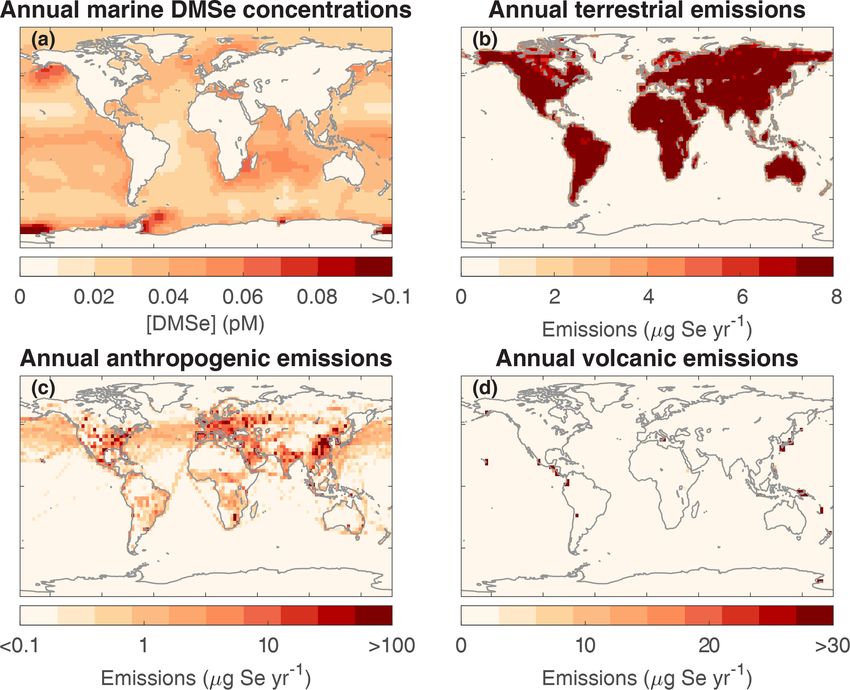
A. Feinberg et al.: Mapping the drivers of uncertainty in atmospheric selenium deposition                                  1365

variables can be neglected; (3) understanding the behavior of      trates the comparison between the compiled Se deposition
the model, for example how the output depends on interac-          measurements and simulated results. A discussion of both
tions between input variables; and (4) identifying possible        sensitivity analyses follows in Sect. 6, and the paper is con-
model bugs or discontinuities, since the model will be tested      cluded in Sect. 7.
with a wide range of input parameter values (Saltelli et al.,
2000; Ryan et al., 2018).
   There are several recent examples of atmospheric chem-          2     Model description
istry studies that included a global sensitivity analysis. The
sensitivity of cloud condensation nuclei number density to         2.1    SOCOL-AER
input parameters in an aerosol model was investigated at the
local (geographic) scale (Lee et al., 2011) and at the global      SOCOL-AERv2 is a global CCM that includes a sulfate
scale (Lee et al., 2012, 2013), revealing regional differences     aerosol microphysical scheme (Sheng et al., 2015; Feinberg
in parameter rankings. Revell et al. (2018) investigated the       et al., 2019b). The base CCM, SOCOLv3 (Stenke et al.,
sensitivity of the tropospheric ozone columns to emission          2013), is a combination of the general circulation model
and chemical parameters, to identify which processes are re-       ECHAM5 (Roeckner et al., 2003) and the chemical model
sponsible for the bias in modeled tropospheric ozone. Mar-         MEZON (Egorova et al., 2003). The MEZON submodel
shall et al. (2019) employed global sensitivity analysis meth-     comprises a comprehensive atmospheric chemistry scheme,
ods to identify how radiative forcing responds to volcanic         with 89 gas-phase chemical species, 60 photolysis reac-
emission parameters. In these examples, surrogate modeling         tions, 239 gas-phase reactions, and 16 heterogeneous reac-
techniques (also known as emulation) were employed to re-          tions. Chemical tracers are advected in the model using the
place a process-oriented, computationally expensive model          Lin and Rood (1996) semi-Lagrangian method. Photolysis
with an approximative statistical model. The statistical model     rates are calculated using a look-up table approach based
has the advantage that it is quicker to evaluate; therefore, it    on the simulated overhead ozone and oxygen columns. The
can be used to calculate the model output throughout the           MEZON model solves the system of differential equations
parametric space (Lee et al., 2011). The examples given            representing chemical reactions with a Newton–Raphson it-
above all used Gaussian process emulation; however other           erative method for short-lived chemical species and an Euler
surrogate modeling techniques exist, including polynomial          method for long-lived species.
chaos expansions (PCEs) (Ghanem and Spanos, 2003). The                The sulfate aerosol model AER (Weisenstein et al., 1997)
PCE approach is well suited to sensitivity analysis, since the     was first coupled to SOCOL by Sheng et al. (2015). SOCOL-
Sobol’ sensitivity indices can be extracted analytically from      AER includes gas-phase S chemistry and 40 sulfate aerosol
the constructed PCE, with no need to evaluate the surrogate        tracers, ranging in dry radius size from 0.39 nm to 3.2 µm.
model through Monte Carlo sampling (Sudret, 2008). This            SOCOL-AER simulates microphysical processes that affect
can greatly reduce the computational time required to con-         the aerosol size distribution, including binary homogeneous
duct the sensitivity analysis, especially when one is inter-       nucleation, condensation of H2 SO4 and H2 O, coagulation,
ested in conducting a separate sensitivity analysis for many       evaporation, and sedimentation. SOCOL-AER was extended
model grid boxes.                                                  in Feinberg et al. (2019b) to include interactive wet and dry
                                                                   deposition schemes. The wet deposition scheme, based on
1.3   Outline                                                      Tost et al. (2006), calculates scavenging of gas-phase species
                                                                   depending on their Henry’s law coefficients and aerosol
This study focuses on the construction of the first global at-     species depending on the particle diameter. The wet removal
mospheric Se model and the insights that this model reveals        of tracers is coupled to the grid cell simulated properties of
into which Se cycle uncertainties would be the most im-            clouds and precipitation. The dry deposition scheme is based
portant to constrain. Section 2 describes the SOCOL-AER            on Kerkweg et al. (2006, 2009), who use the surface resis-
(modeling tools for studies of SOlar Climate Ozone Links –         tance approach of Wesely (1989). In addition to surface type
aerosol) model and the implementation of Se chemistry in the       and meteorology, the calculated dry deposition velocities de-
SOCOL-AER model. The SOCOL-AER model is a suitable                 pend on reactivity and solubility for gas-phase compounds
tool to model the Se cycle, since it successfully describes the    and size for aerosol species. SOCOL-AER uses an opera-
major properties of the atmospheric S cycle (Sheng et al.,         tor splitting approach, wherein the model time step is 2 h for
2015; Feinberg et al., 2019b). The statistical methods that        chemistry and radiation and 15 min for dynamics and depo-
we use to conduct the sensitivity analysis are discussed in        sition. Aerosol microphysical routines use a sub-time step of
Sect. 3. Section 4 details the methods used to compile a           6 min.
database of measured wet Se deposition fluxes, which we use           For the simulations in this study we use boundary con-
to evaluate the model. The results of the sensitivity analy-       ditions for the year 2000. Sea ice coverage and sea surface
ses are presented in Sect. 5.1 for the atmospheric Se lifetime     temperatures are prescribed from the Hadley Centre dataset
and Sect. 5.2 for the Se deposition patterns. Section 5.3 illus-   (Rayner et al., 2003). The year 2000 concentrations of the

www.atmos-chem-phys.net/20/1363/2020/                                               Atmos. Chem. Phys., 20, 1363–1390, 2020
1366                            A. Feinberg et al.: Mapping the drivers of uncertainty in atmospheric selenium deposition

most relevant greenhouse gases (CO2 , CH4 , and N2 O) de-           1993; Wen and Carignan, 2007). A variety of methylated Se
rive from NOAA observations (Eyring et al., 2008). Anthro-          species have been observed from biogenic emissions, includ-
pogenic CO and NOx emissions are based on the RETRO                 ing DMSe, dimethyl diselenide (DMDSe), dimethyl selenyl-
dataset (Schultz and Rast, 2007), while natural emissions           sulfide (DMSeS), and methane selenol (MeSeH) (Amouroux
are taken from Horowitz et al. (2003). Sulfur dioxide (SO2 )        and Donard, 1996, 1997; Amouroux et al., 2001; Wen and
emissions from anthropogenic sources follow the year 2000           Carignan, 2007). Since DMSe is usually the dominant emit-
inventory from Lamarque et al. (2010) and Smith et al.              ted compound, and little is known about the oxidation ki-
(2011). Volcanic degassing SO2 emissions are assigned to            netics of the other methylated species, DMSe is the only
surface grid boxes where volcanoes are located (Andres and          species emitted by marine and terrestrial biogenic emissions
Kasgnoc, 1998; Dentener et al., 2006). Atmospheric emis-            in SOCOL-AER.
sions of dimethyl sulfide (DMS) are calculated using a wind-           Atmospheric S emissions have been measured more exten-
based parametrization (Nightingale et al., 2000) and a marine       sively than Se emissions, so we scale inventories of S emis-
DMS climatology (Lana et al., 2011). To represent mean con-         sions to yield the spatial distribution of emitted Se. For the
ditions for photolysis, the look-up table for photolysis rates      sensitivity analysis we assume that the Se emissions have the
is averaged over two solar cycles (1977–1998).                      same distribution as S emissions, and we focus on the un-
                                                                    certainties in the global scaling factors for each source. The
2.2     Implementing Se emissions and chemistry in                  range in scaling factors will be discussed in Sect. 3.1.4. The
        SOCOL-AER                                                   spatial distribution of anthropogenic and biomass burning Se
                                                                    emissions comes from the SO2 inventory for the year 2000
2.2.1    Selenium species overview                                  (Lamarque et al., 2010; Smith et al., 2011). For sea surface
                                                                    DMSe concentrations, we scale the DMS climatology cal-
We included the Se cycle in SOCOL-AER (Fig. 1) based on             culated by Lana et al. (2011). We determine DMSe emis-
the existing literature on atmospheric Se (Ross, 1985; Wen          sions using a wind-driven parametrization (Nightingale et al.,
and Carignan, 2007). Seven Se gas-phase tracers have been           2000). The locations and strength of background degassing
added to SOCOL-AER (Table 1): carbonyl selenide (OCSe),             volcanic emissions are taken from the Global Emissions Ini-
thiocarbonyl selenide (CSSe), carbon diselenide (CSe2 ),            tiAtive (GEIA) inventory (Andres and Kasgnoc, 1998; Den-
dimethyl selenide (DMSe), hydrogen selenide (H2 Se), ox-            tener et al., 2006). Since little is known about both terres-
idized inorganic Se (OX_Se_IN), and oxidized organic Se             trial biogenic Se emissions and terrestrial S emissions (Pham
(OX_Se_OR). The oxidized inorganic Se tracer represents             et al., 1995), we assume that terrestrial Se is emitted in all
species such as elemental Se, selenium dioxide (SeO2 ), se-         land surface grid boxes, excluding glaciated locations.
lenous acid (H2 SeO3 ), and selenic acid (H2 SeO4 ). Very lit-
tle is known about the kinetics of interconversion between          2.2.3   Chemistry of Se species
the oxidized inorganic Se species (Wen and Carignan, 2007),
and therefore in our model they are treated as one tracer.          We conducted a literature review to develop the model’s
However, these species all have very low vapor pressures un-        chemical scheme of the Se cycle. Reactions of Se species
der atmospheric conditions (Rumble, 2017) and likely par-           that have been measured by laboratory studies are compiled
tition to the particulate phase. Oxidized organic Se species        in Table 2. We neglect any temperature dependency in the
include dimethyl selenoxide (DMSeO) and methylseleninic             Se reaction rates, since the Se reactions have only been
acid (CH3 SeO2 H), which form after oxidation of DMSe               studied at around 298 K. For all compiled reactions, atmo-
(Atkinson et al., 1990; Rael et al., 1996). Similar to the oxi-     spheric Se compounds react much quicker than the analo-
dized inorganic Se compounds, oxidized organic Se species           gous S compounds, due to the stronger bonds that S forms
also partition to the particulate phase due to their low volatil-   with carbon and hydrogen than Se (Rumble, 2017). In ad-
ities (Rael et al., 1996).                                          dition, there are reactions that are known to occur for the
                                                                    analogous S compound, but have never been studied for the
2.2.2    Selenium emissions                                         Se compound (OCSe + OH, CSSe + OH, CSe2 + OH, and
                                                                    H2 Se + OH). These reaction rate constants were estimated
To determine which Se compounds are emitted by the differ-          in Fig. 2, which shows the ratio of the Se compounds’ rates
ent sources, we have reviewed studies that investigated the         to analogous S rates (i.e., an enhancement factor for replac-
speciation of Se emissions. Thermodynamic modeling and              ing an S atom with Se) plotted versus the S reaction rate. For
in situ measurements of combustion exhaust gases have de-           S reactions which have a fast reaction rate (e.g., DMS + Cl,
tected the following Se species in anthropogenic emissions:         k = 1.8×10⁻¹⁰ cm3 molec.−1 s−1 ), replacing S with Se does
oxidized inorganic Se, H2 Se, OCSe, CSe2 , and CSSe (Yan            not yield a large difference in measured rates (DMSe + Cl,
et al., 2000, 2004; Pavageau et al., 2002, 2004). Oxidized in-      k = 5.0 × 10⁻¹⁰ cm3 molec.−1 s−1 ). This is because these re-
organic Se species and minor amounts of H2 Se are expected          actions are already close to the collision-controlled limit, and
to be emitted from volcanic degassing (Symonds and Reed,            thus lowering the activation energy by substituting a Se atom

Atmos. Chem. Phys., 20, 1363–1390, 2020                                              www.atmos-chem-phys.net/20/1363/2020/
A. Feinberg et al.: Mapping the drivers of uncertainty in atmospheric selenium deposition                                          1367

Figure 1. Scheme of the atmospheric Se cycle in SOCOL-AER, based on information in Ross (1985) and Wen and Carignan (2007). For
simplicity the two oxidized Se tracers in SOCOL-AER are represented with a single box. The impact on agriculture and human health is also
shown, since it motivates the study of atmospheric Se.

Table 1. Description of Se tracers included in SOCOL-AER.

  Abbreviation    Name                           Sources                                                       Sinks
  OCSe            Carbonyl selenide              Anthropogenic emissions, chemical production                  Chemical loss
  CSSe            Thiocarbonyl selenide          Anthropogenic emissions                                       Chemical loss
  CSe2            Carbon diselenide              Anthropogenic emissions                                       Chemical loss
  DMSe            Dimethyl selenide              Marine and terrestrial emissions                              Chemical loss
  H2 Se           Hydrogen selenide              Anthropogenic and volcanic emissions                          Chemical loss
  OX_Se_IN        Oxidized inorganic Se          Anthropogenic and volcanic emissions, chemical production     Dry and wet deposition
  OX_Se_OR        Oxidized organic Se            Anthropogenic and volcanic emissions, chemical production     Dry and wet deposition
  –               Se in S aerosol (40 tracers)   Uptake of gas-phase oxidized Se                               Dry and wet deposition
  –               Se in dummy aerosol            Uptake of gas-phase oxidized Se                               Dry and wet deposition

for S has little impact on the overall rate. On the other hand,        measured, however in too low resolution to be incorporated
slow reactions like DMS+O3 are sped up by more than 4 or-              into the model. Therefore, we assume that CSe2 and CSSe
ders of magnitude when Se is substituted for S. We used the            have the same cross section as CS2 (Burkholder et al., 2015).
log-log relationship in Fig. 2 to predict the reaction rates for       Given the lack of available information, quantum yields for
OCSe, CSSe, and H2 Se with OH (blue stars). The CSe2 reac-             all Se photolysis reactions were assumed to be 1.
tion with OH is calculated from the CSSe reaction, assuming
an enhancement for the substitution of a second Se atom sim-           2.2.4   Condensation of Se on preexisting aerosol
ilar to that between the measured CSe2 + O and CSSe + O                        particles
reaction rates (Li et al., 2005). The branching ratio for the
CSSe+OH reaction products was assumed to be 30 % OCSe                  As nonvolatile species, oxidized inorganic and organic Se
and 70 % OX_Se_IN, the same as the measured CSSe + O                   would condense on available atmospheric surfaces. In the
branching ratio (Li et al., 2005). We recognize that these es-         SOCOL-AER model, the uptake of these oxidized Se species
timates are inherently uncertain, and therefore we address             by sulfate aerosols is calculated similarly to the existing
these uncertainties in our sensitivity analysis (Sect. 3.1.2).         scheme of gas-phase H2 SO4 uptake on sulfate particles
   The photolysis of gas-phase Se compounds was included               (Sheng et al., 2015). We track the size distribution of Se
using absorption cross sections of H2 Se (Goodeve and Stein,           in the aerosol phase with 40 tracers, one for each sulfate
1931) and OCSe (Finn and King, 1975). The absorption cross             aerosol size bin. The sulfate aerosol size distribution changes
section of CSe2 (King and Srikameswaran, 1969) has been                through processes like growth, evaporation, and coagula-
                                                                       tion. We track how these microphysical processes change the

www.atmos-chem-phys.net/20/1363/2020/                                                    Atmos. Chem. Phys., 20, 1363–1390, 2020
1368                             A. Feinberg et al.: Mapping the drivers of uncertainty in atmospheric selenium deposition

Table 2. Rate constants of Se compound gas-phase reactions at around 298 K and the corresponding rate constant of the analogous S
compound. All S reaction rates are from Burkholder et al. (2015), except the DMS+ O3 reaction rate which is taken from Wang et al. (2007).
No corresponding rate constants for CSe2 reactions are listed, since CSe2 is obtained from doubly substituting Se in CS2 .

       Reaction                                      Se rate constant       Corresponding S constant   Reference for Se
                                                  (cm3 molec.−1 s−1 )            (cm3 molec.−1 s−1 )   rate constant
       Measured reactions
       OCSe + O → CO + OX_Se_IN                           2.4 × 10⁻¹¹                   1.3 × 10⁻¹⁴    Li et al. (2005)
       CSe2 + O → OCSe + OX_Se_IN (32 %)                                                               Li et al. (2005)
                                                          1.4 × 10⁻¹⁰                              –
            → 2 OX_Se_IN (68 %)
       CSSe + O → OCSe (30 %)                             2.8 × 10⁻¹¹                   3.6 × 10⁻¹²    Li et al. (2005)
             → OX_Se_IN (70 %)
       DMSe + OH → OX_Se_OR                               6.8 × 10⁻¹¹                   6.7 × 10⁻¹²    Atkinson et al. (1990)
       DMSe + NO3 → OX_Se_OR                              1.4 × 10⁻¹¹                   1.1 × 10⁻¹²    Atkinson et al. (1990)
       DMSe + O3 → OX_Se_OR                               6.8 × 10⁻¹⁷                   2.2 × 10⁻²¹    Atkinson et al. (1990)
       DMSe + Cl → OX_Se_OR                               5.0 × 10⁻¹⁰                   1.8 × 10⁻¹⁰    Thompson et al. (2002)
       H2 Se + O → OX_Se_IN                               2.1 × 10⁻¹²                   2.2 × 10⁻¹⁴    Agrawalla and Setser (1987)
       H2 Se + Cl → OX_Se_IN                              5.5 × 10⁻¹⁰                   7.4 × 10⁻¹¹    Agrawalla and Setser (1986)
       H2 Se + O3 → OX_Se_IN                              3.2 × 10⁻¹⁶                 < 2.0 × 10⁻²⁰    Belyaev et al. (2012)
       Estimated reactions
       OCSe + OH → OX_Se_IN                               5.8 × 10⁻¹³                   2.0 × 10⁻¹⁵    Estimated; see text.
       CSe2 + OH → OCSe + OX_Se_IN                        1.5 × 10⁻¹⁰                             –    Estimated; see text.
       CSSe + OH → OX_Se_IN (70 %)                        3.0 × 10⁻¹¹                   1.2 × 10⁻¹²
                                                                                                       Estimated; see text.
            → OCSe (30 %)
       H2 Se + OH → OX_Se_IN                              7.2 × 10⁻¹¹                   4.7 × 10⁻¹²    Estimated; see text.

size distribution of condensed Se through mass-conserving               magnitude of these particles (Sect. 3.1.7), we can determine
schemes. Evaporation of condensed Se only occurs when                   whether missing aerosols affect atmospheric Se cycling.
the smallest sulfate aerosol bin evaporates, releasing the Se
stored in that bin as gas-phase inorganic oxidized Se. Sedi-
mentation and deposition of the host sulfate particles are con-         3    Statistical methods
current with sedimentation and deposition of the condensed
                                                                        To conduct the sensitivity analysis of our Se model, we first
Se tracers. Gas-phase oxidized Se tracers are also removed
                                                                        need to select the input parameters that would be included in
by dry and wet deposition, with the assumption that they have
                                                                        the sensitivity analysis. The probability distributions of these
the same Henry’s law constant as gas-phase H2 SO4 .
                                                                        input parameters’ uncertainties were determined by review-
   One limitation of using SOCOL-AER for the Se cycle is
                                                                        ing literature sources and using our best judgment. Variance-
that the model only includes online sulfate aerosols. This
                                                                        based sensitivity analysis methods usually require 104 to 106
means that the transport of Se on other aerosols, including
                                                                        model runs, which would be prohibitively expensive for the
dust, sea salt, and organic aerosols, would be neglected. This
                                                                        full SOCOL-AER model. We therefore replace the SOCOL-
may not be a poor assumption, since Se and S are often co-
                                                                        AER model with a surrogate PCE model. The SOCOL-AER
emitted and have been found to be highly correlated in at-
                                                                        model is run at carefully selected points within the parame-
mospheric aerosol measurements (e.g., Eldred, 1997; Weller
                                                                        ter space, creating a set of “training” runs. The training runs
et al., 2008). Nevertheless, we included a “dummy” aerosol
                                                                        are used to produce a surrogate PCE model, which approx-
tracer to test the effect of missing aerosol species in SOCOL-
                                                                        imates the outputs of the full SOCOL-AER model through-
AER. The dummy aerosol tracer represents monodisperse
                                                                        out the input parameter space. Sensitivity indices can then
particles that are emitted in a latitudinal band in the model
                                                                        be derived from the surrogate model. All statistical methods
and undergo Se uptake, sedimentation, and wet and dry depo-
                                                                        presented in this section are available in UQL AB, an open-
sition. This dummy aerosol tracer is clearly a simplification
                                                                        source MATLAB-based framework for uncertainty quantifi-
of true atmospheric processes, as in reality other aerosols are
                                                                        cation (Marelli and Sudret, 2014).
distributed in size and can coagulate with sulfate aerosol par-
ticles. However, by varying the radius, location, and emission

Atmos. Chem. Phys., 20, 1363–1390, 2020                                                    www.atmos-chem-phys.net/20/1363/2020/
A. Feinberg et al.: Mapping the drivers of uncertainty in atmospheric selenium deposition 1369
Figure 2. Estimation of unknown Se reaction rates from the analogous S reaction rate. A power regression is performed, with statistics shown
in the upper right corner of the plot. For the H2 S + O3 reaction only an upper limit estimate was available, and therefore it was not included
in the analysis.
3.1 Uncertainty ranges of input parameters been measured in six studies (Atkinson et al., 1978; Kurylo,
1978; Cox and Sheppard, 1980; Leu and Smith, 1981; Cheng
We restricted the scope of our sensitivity analysis to param- and Lee, 1986; Wahner and Ravishankara, 1987; Burkholder
eters that have been implemented in the model as part of et al., 2015). The measured reaction rate constant varied over
the Se cycle. We neglect other model parameters, including multiple orders of magnitude; therefore, we calculated its
those related to climate, deposition parametrizations, or the variability on a logarithmic scale. The coefficient of vari-
emissions of sulfate aerosol precursors. The focus of our sen- ation (standard deviation divided by mean) of this reaction
sitivity analysis is to prioritize which Se-related parameters rate in logarithmic space was around 6 %. We assumed that
should be further constrained. Since we do not vary all other this maximum S coefficient of variation would apply to the
model parameters, the uncertainties of output quantities may measured Se reaction rates. The bounds were calculated as
be underestimated. However, given the large dimension of 88 % and 112 % (±2 standard deviations) of the available
our parameter space with 34 Se-related input parameters, in- measured rate constant in logarithmic space, i.e.,
cluding additional non-Se-related parameters would be chal-
lenging. In the following section, we will discuss the uncer- bounds = k 1±0.12 , (1)
tainty distributions for each of the 34 input parameters in- where k is the measured rate constant and “bounds” are its
cluded in our study. Due to the lack of detailed information upper and lower bounds, all expressed in cubic centimeters
available in literature about the parameter distributions, we per molecule per second. The maximum upper bound was set
chose loguniform or uniform distributions for all but one of to 1.0 × 10⁻⁹ cm3 molec.−1 s−1 , since at this order of magni-
the parameters. This follows the conservative approach rec- tude the Se reaction rates are collision-limited (Seinfeld and
ommended by the maximum entropy principle, as the uni- Pandis, 2016).
form and loguniform distributions maximize entropy while
fulfilling the data constraints (Kapur, 1989). The uncertainty 3.1.2 Estimated rate constants (k13 –k17 )
distributions of all input parameters are listed in Table 3.
Five Se reaction rate constants have not been measured pre-
3.1.1 Measured rate constants (k1 –k12 ) viously in the laboratory and were estimated based on their
relationship with analogous S rate constants (Fig. 2). We cal-
The Se reactions studied in the literature each have only culated the uncertainty bounds of estimated rate constants
been measured by one laboratory group (Table 2). Since only using the 95 % error interval of prediction with a linear re-
one measurement technique has been applied, the reported gression (Wackerly et al., 2014):
measurement uncertainties may underestimate the true un- v !
2
u
certainties of these rate constants. To approximate an uncer- u SSE 1 (x − x) , (2)
bounds = 10 x + Ŷ ± t0.025 t 1+ +
tainty distribution for these rate constants, we reviewed S n−2 n Sxx
compound reactions that have been studied by multiple re-
search groups. The reaction that had the largest spread in re- where x is the logarithm (to the base 10) of the corresponding
ported rate constants at ∼ 298 K was OCS + OH, which has S rate constant, Ŷ is the logarithm of the predicted ratio of
www.atmos-chem-phys.net/20/1363/2020/ Atmos. Chem. Phys., 20, 1363–1390, 2020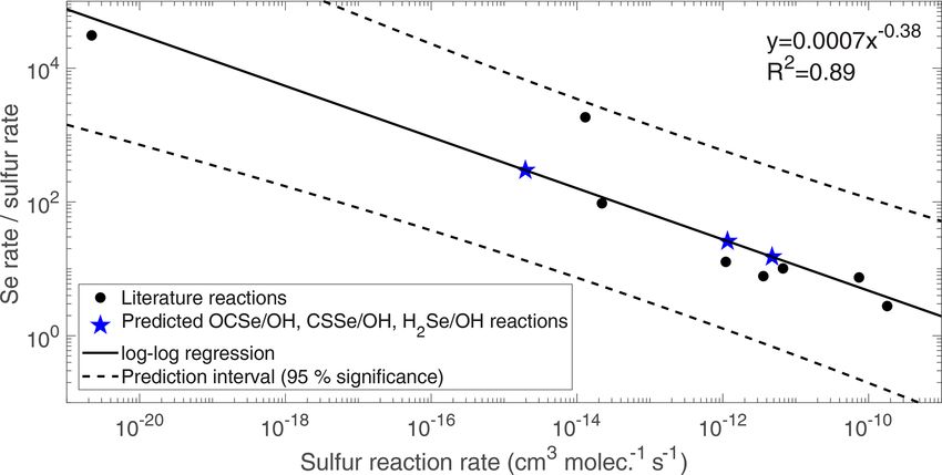
1370                              A. Feinberg et al.: Mapping the drivers of uncertainty in atmospheric selenium deposition

Table 3. Probability distributions of the model input parameters selected for the sensitivity analysis.

       Input parameter     Description                                           Lower bound       Upper bound    Distribution
       Measured reaction rate coefficients (cm3 molec.−1 s−1 )
       k1                  OCSe + O → CO + OX_Se_IN                               1.3 × 10⁻¹²      4.5 × 10⁻¹⁰    loguniform
       k2                  CSe2 + O → OCSe + OX_Se_IN                             2.6 × 10⁻¹²      7.8 × 10⁻¹⁰    loguniform
       k3                  CSe2 + O → 2 OX_Se_IN                                  6.0 × 10⁻¹²       1.0 × 10⁻⁹    loguniform
       k4                  CSSe + O → OCSe                                        4.0 × 10⁻¹³      1.8 × 10⁻¹⁰    loguniform
       k5                  CSSe + O → OX_Se_IN                                    1.0 × 10⁻¹²      3.8 × 10⁻¹⁰    loguniform
       k6                  DMSe + OH → OX_Se_OR                                   4.1 × 10⁻¹²       1.0 × 10⁻⁹    loguniform
       k7                  DMSe + NO3 → OX_Se_OR                                  7.0 × 10⁻¹³      2.8 × 10⁻¹⁰    loguniform
       k8                  DMSe + O3 → OX_Se_OR                                   7.8 × 10⁻¹⁹      5.9 × 10⁻¹⁵    loguniform
       k9                  DMSe + Cl → OX_Se_OR                                   3.8 × 10⁻¹¹       1.0 × 10⁻⁹    loguniform
       k10                 H2 Se + O → OX_Se_IN                                   8.3 × 10⁻¹⁴      5.3 × 10⁻¹¹    loguniform
       k11                 H2 Se + Cl → OX_Se_IN                                  4.6 × 10⁻¹¹       1.0 × 10⁻⁹    loguniform
       k12                 H2 Se + O3 → OX_Se_IN                                  4.4 × 10⁻¹⁸      2.3 × 10⁻¹⁴    loguniform
       Estimated reaction rate coefficients (cm3 molec.−1 s−1 )
       k13                 OCSe + OH → OX_Se_IN                                   2.6 × 10⁻¹⁴      1.3 × 10⁻¹¹    loguniform
       k14                 CSe2 + OH → OCSe + OX_Se_IN                            7.0 × 10⁻¹²       1.0 × 10⁻⁹    loguniform
       k15                 CSSe + OH → OX_Se_IN                                   9.8 × 10⁻¹³      4.5 × 10⁻¹⁰    loguniform
       k16                 CSSe + OH → OCSe                                       4.2 × 10⁻¹³      1.9 × 10⁻¹⁰    loguniform
       k17                 H2 Se + OH → OX_Se_IN                                  3.3 × 10⁻¹²       1.0 × 10⁻⁹    loguniform
       Scaling factors for photolysis rates
       f k18               OCSe + hν → OX_Se_IN                                               0              2    uniform
       f k19               CSe2 + hν → 2 OX_Se_IN                                             0              2    uniform
       f k20               CSSe + hν → OX_Se_IN                                               0              2    uniform
       f k21               H2 Se + hν → OX_Se_IN                                              0              2    uniform
       Global emission by source category (Gg Se yr−1 )
       emissmar            Marine biogenic Se emissions                                     0.4             35    loguniform
       emissterr           Terrestrial biogenic Se emissions                              0.15            5.25    uniform
       emissant            Anthropogenic Se emissions                                         3            9.6    uniform
       emissvol            Volcanic Se emissions                                         0.076            49.1    loguniform
       Speciation of emissions (%)
       %OCSeant            OCSe fraction in anthropogenic emissions                           0              6    uniform
       %CSe2ant            CSe2 fraction in anthropogenic emissions                           0              6    uniform
       %CSSeant            CSSe fraction in anthropogenic emissions                           0              6    uniform
       %H2 Seant           H2 Se fraction in anthropogenic emissions                          0              6    uniform
       %H2 Sevol           H2 Se fraction in volcanic emissions                               0             13    uniform
       Accommodation coefficient
       acccoeff            Oxidized Se uptake on aerosols                                  0.02              1    uniform
       Dummy aerosol parameters
       raer                Radius of missing aerosol (µm)                                  0.01               3   loguniform
       emissaer            Emission magnitude of missing aerosol (kg yr−1 )                   –               –   lognormal (see text)
       lataer              Latitudinal band of aerosol emission                     90 to 80◦ S     80 to 90◦ N   uniform

Atmos. Chem. Phys., 20, 1363–1390, 2020                                                       www.atmos-chem-phys.net/20/1363/2020/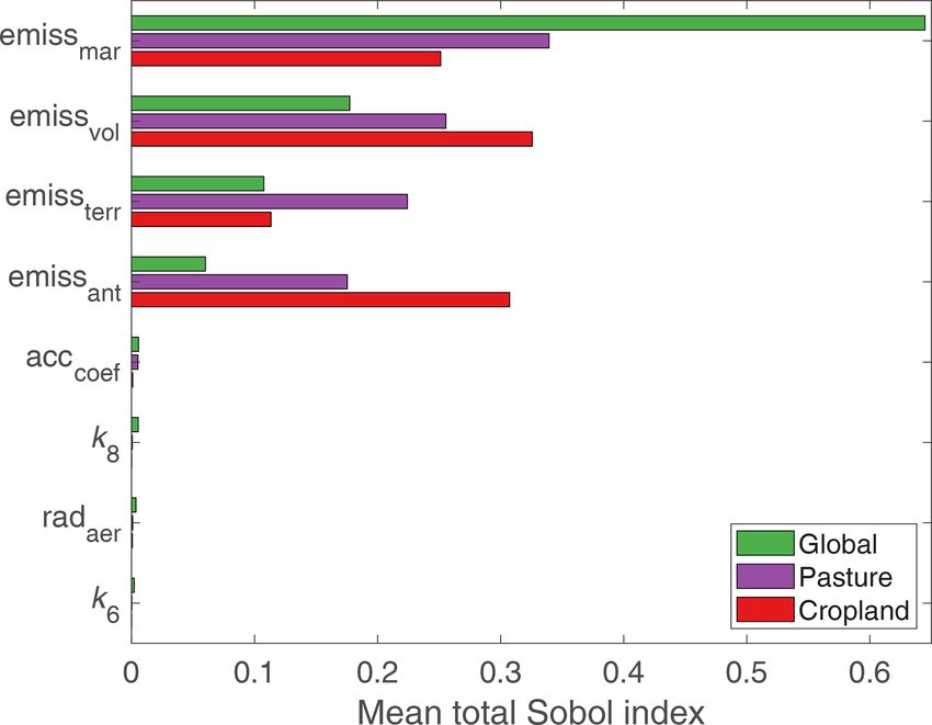
A. Feinberg et al.: Mapping the drivers of uncertainty in atmospheric selenium deposition 1371
the Se rate to the S rate, n is the number of data points in the degassing SO2 emissions from Andres and Kasgnoc (1998)
regression, t0.025 is the 2.5th percentile value of the Student and Dentener et al. (2006), 12.6 Tg S yr−1 , we calculate an
t distribution for n − 2 degrees of freedom, x is the mean of uncertainty range for total volcanic Se emissions: 0.076–
the logarithm of S rate constants in Fig. 2, SSE is the sum of 49.1 Gg Se yr−1 . Loguniform distributions were used for the
squares of the residuals, and Sxx is the variance of the S rate source types whose total emission ranges vary by more than 2
constants in Fig. 2. All rate constants are in units of cubic orders of magnitude (volcanic and marine biogenic), whereas
centimeters per molecule per second. uniform distributions were used for the terrestrial and anthro-
pogenic Se emissions.
3.1.3 Photolysis rate scaling factors
3.1.5 Speciation of Se emission sources
Uncertainties in our calculated Se photolysis rates arise from
uncertainties in the measured OCSe and H2 Se cross sections,
The available speciation information for Se emissions is
the assumption that CSe2 and CSSe have the same cross sec-
largely qualitative; possible emission species have been iden-
tion as CS2 , the quantum yields of photolysis reactions, and
tified but not quantified (Sect. 2.2.2). To estimate the uncer-
the look-up table approach that SOCOL-AER applies to cal-
tainty range for Se emission speciation, we use estimates of
culate photolysis rates. Given the lack of specific informa-
speciation from an atmospheric S budget (Watts, 2000). The
tion about these uncertainties, we apply a scaling factor on
second most important anthropogenic S species after SO2
the calculated photolysis rates ranging from 0 to 2 (Table 3).
is H2 S. Watts (2000) estimates the anthropogenic emission
of H2 S is 3.1 ± 0.3 Tg S yr−1 , compared to an anthropogenic
3.1.4 Global emissions from source categories
SO2 emission total of 53.2 Tg S yr−1 (Lamarque et al., 2010;
Smith et al., 2011) in the year 2000. H2 S therefore con-
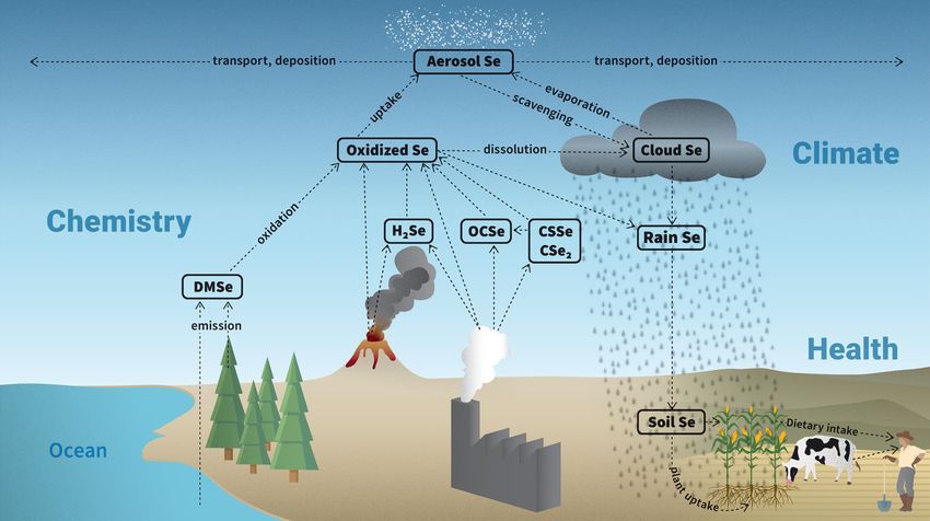
For the sensitivity analysis, we do not alter the spatial dis-
tributes at most 6 % of total S emissions. Since OCSe, CSe2 ,
tribution of Se emissions from anthropogenic, marine bio-
CSSe, and H2 Se are in general less stable than the analo-
genic, terrestrial biogenic, and volcanic sources (Fig. 3). The
gous S species (Table 2), we consider 6 % to be a maximum
parameters that we varied are the scaling factors for each
value for the mass fraction of anthropogenic Se emissions
map, i.e., the global total emissions from each source. We
that come from each of these species. The anthropogenic spe-
reviewed atmospheric Se budget estimates to determine the
ciation fractions for OCSe, CSe2 , CSSe, and H2 Se are varied
range in total emissions for different sources (Table S1).
between 0 % and 6 %. The rest of the anthropogenic emis-
The estimates for global DMSe emissions ranged from the
sions, 76 %–100 %, are attributed to OX_Se_IN, representing
lower limit value of 0.4 Gg Se yr−1 in Nriagu (1989) to
species such as Se and SeO2 .
35 Gg Se yr−1 in Amouroux et al. (2001). DMSe emissions
Regarding the speciation of volcanic S emissions, Watts
are calculated online in the model from a marine DMSe con-
(2000) estimates that 0.99 ± 0.88 Tg S yr−1 is in the form of
centration map. Based on the results of a previous simulation,
H2 S. Comparing this to the estimate for volcanic SO2 emis-
we normalize the marine DMSe concentration map in Fig. 3a
sions, 12.6 Tg S yr−1 (Andres and Kasgnoc, 1998; Dentener
so that it leads to 1 Gg Se yr−1 emissions globally. All other
et al., 2006), H2 S contributes at most 13 % of volcanic S
maps are also normalized to 1 Gg Se yr−1 emissions, so that
emissions. Therefore, in our sensitivity analysis the percent-
we can directly apply the total global emissions as a scaling
age of volcanic Se emissions in the form of H2 Se ranges from
factor. The widest uncertainty range of terrestrial emissions
0 % to 13 %. Conversely, the percentage of OX_Se_IN in vol-
was given by Nriagu (1989), from 0.15 to 5.25 Gg Se yr−1 .
canic emissions ranges from 87 % to 100 %.
Total global anthropogenic Se emissions in 1983 were esti-
mated between 3.0 and 9.6 Gg Se yr−1 (Nriagu and Pacyna,
1988). We applied the same uncertainty range to the total an- 3.1.6 Accommodation coefficient of oxidized Se
thropogenic emissions in the year 2000, because it is unclear
how global Se emissions have changed during this period. To The accommodation coefficient represents the probability
estimate global Se emissions from degassing volcanoes, we that a gas-phase oxidized Se molecule will stick to an aerosol
reviewed measurements of Se-to-S ratios in volcanic emis- particle upon collision. No laboratory studies have inves-
sions, extending the studies reviewed in Floor and Román- tigated the accommodation coefficient of oxidized Se on
Ross (2012) (Table S2 in the Supplement). There is a high aerosol surfaces. However, review papers suggest that Se
degree of variability in the emitted Se-to-S ratios between efficiently partitions to the aerosol phase upon oxidation
different volcanoes, and even temporally and spatially for the (Mosher and Duce, 1987; Wen and Carignan, 2007), indi-
same volcano (Floor and Román-Ross, 2012). The Se-to-S cating a high accommodation coefficient. Due to the lack of
ratio in volcanic emissions ranges from 6 × 10⁻⁶ for White further information, we assume an uncertainty range of 0.02–
Island, New Zealand (Wardell et al., 2008), to 3.9 × 10⁻³ 1 for the accommodation coefficient, as selected by Lee et al.
for Merapi Volcano, Indonesia (Symonds et al., 1987). By (2011) for H2 SO4 . This accommodation coefficient applies
multiplying this range in ratios with the global mean total to uptake of Se on sulfate and dummy aerosols.
www.atmos-chem-phys.net/20/1363/2020/ Atmos. Chem. Phys., 20, 1363–1390, 2020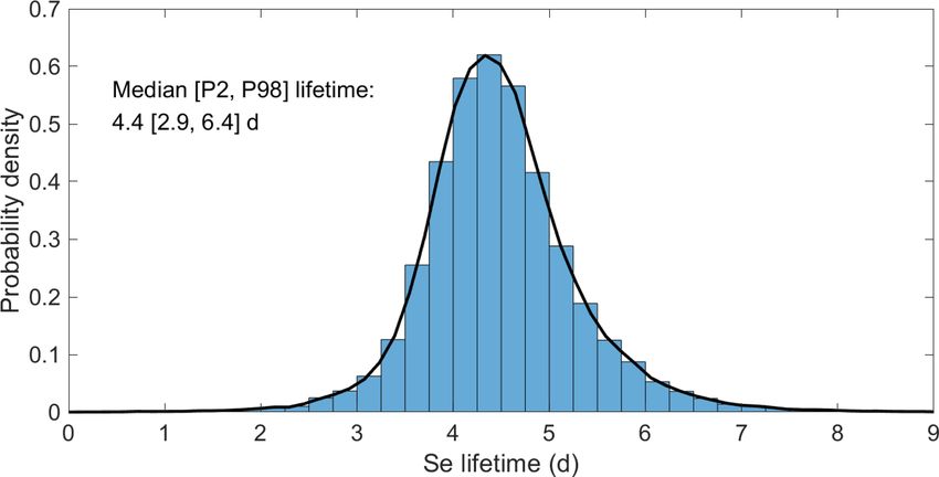
1372                             A. Feinberg et al.: Mapping the drivers of uncertainty in atmospheric selenium deposition

Figure 3. Spatial distribution of Se sources. Each source map is normalized so that 1 Gg Se yr−1 would be emitted globally. This is scaled
during the sensitivity analysis.

3.1.7   Dummy aerosol tracers                                          tener et al., 2006). Aerosol types are segregated into size
                                                                       classes based on their effective radius, and the emission mag-
SOCOL-AER only includes sulfate aerosol, lacking other                 nitude for 10◦ latitude bands is calculated for each size class.
aerosol types (e.g., dust, sea salt, organic aerosol) that may         The mass emission of particles correlates with the particle
also transport Se. To test how these other aerosol types might         size, with generally larger mass emissions for larger parti-
affect Se transport and deposition, in the sensitivity analy-          cle sizes (Fig. S1 in the Supplement). Therefore, the value
sis we vary the emission location, particle radius, and emis-          of emission magnitude in our experiments depends lognor-
sion magnitude of the dummy aerosol tracer (introduced in              mally on the particle radius (r), with mean µ = 2.54r + 19.0
Sect. 2.2.4). These input parameters are different from other          and standard deviation σ = 2.88. We acknowledge that in the
uncertainties, in that they are intended to investigate a lack         real atmosphere particles are emitted globally as size distri-
of model completeness rather than uncertainties in measur-             butions, not monodisperse particles in one latitudinal band.
able quantities. In our experiments the aerosols are emitted in        Nevertheless, by including these input parameters as part of
one of 18 latitude bands, ranging from 90–80◦ S to 80–90◦ N.           the sensitivity analysis, we can identify whether the lack of
The latitude parameter can demonstrate whether Se deposi-              tropospheric aerosols other than sulfate impacts the simu-
tion is affected by these missing aerosol types only in certain        lated Se deposition maps in SOCOL-AER.
latitudinal bands. The emission radius affects the transport
of Se on these missing particles, since the atmospheric life-          3.2   Experimental setup and model outputs
time of these particles depends on radius (Seinfeld and Pan-
dis, 2016). For example, additional coarse particles (radius           The creation of surrogate models requires a set of training
> 1 µm) could inhibit far-range Se transport, since they sed-          runs with the full SOCOL-AER model. The values of the in-
iment and are removed quicker than the accumulation mode               put parameters are varied simultaneously between training
sulfate particles. We vary the emission radius between 0.01            runs, so that interactions between parameters can also be de-
and 3 µm, as this covers the range of atmospherically relevant         tected. A Latin hypercube design is used to draw N samples
particle sizes.                                                        from an M-dimensional input parameter space. In Latin hy-
   To determine a reasonable range for the emission magni-             percube sampling, each parameter range is divided into N
tude of additional aerosol particles, we analyzed the particle         equally probable subintervals. N values for each parameter
emission inventories from the AEROCOM I project (Den-                  are drawn randomly from within each subinterval. The se-

Atmos. Chem. Phys., 20, 1363–1390, 2020                                                  www.atmos-chem-phys.net/20/1363/2020/
A. Feinberg et al.: Mapping the drivers of uncertainty in atmospheric selenium deposition 1373
lected values for all input parameters are then matched ran- 3.3 Surrogate modeling with PCE
domly with each other, to yield N points that cover the pa-
rameter space better than purely random Monte Carlo sam- Sudret (2008) provided a detailed description of using PCE
pling (McKay et al., 1979). The general rule of thumb is to to build surrogate models, which was updated by Le Gratiet
select around 10M training simulations, to adequately cover et al. (2017). We will summarize the most important features
the sample space (Loeppky et al., 2009). We ran N = 400 of the approach here. For this study, a certain output of the
training simulations in our sensitivity analysis with 34 in- SOCOL-AER model (Y ) can be thought of as a finite vari-
put parameters. Producing training simulations from the full ance random variable which is a function of the M = 34 in-
SOCOL-AER model is the most computationally expensive put parameters (X = [X1 , X2 , . . ., X34 ]):
step in the uncertainty and sensitivity analysis. With 48 cores, Y = M(X). (3)
each training run takes around 14 h, corresponding to around
109 core seconds for 400 training simulations. The input X ∈ RM is modeled by a joint probability density
The initial conditions file for the training runs was cre- function (PDF) Q fX whose marginals are assumed indepen-
ated from a previous 10-year spinup of the model under dent, i.e., fX = M i=1 fXi (xi ).
year 2000 conditions. The atmospheric mixing ratios of Se In polynomial chaos decomposition, the output variable Y
tracers are initially set to 0 in each simulation. The simula- is decomposed into the following infinite series (Ghanem and
tions are 18 months long, with the first 6 months considered Spanos, 2003):
to be an equilibration period for the Se tracers. Therefore, we X
Y= yα 9α (X), (4)
analyze only the last 12 months of the 18-month simulation.
α=NM
The model is run with T42 horizontal resolution (approxi-
mately 2.8◦ × 2.8◦ or 300 km × 300 km in latitude and lon- where yα are coefficients to be determined and α is a multi-
gitude) with 39 vertical levels up to 0.01 hPa (∼ 80 km). The index set that defines the degree
Q of the multivariate orthonor-
interactions between chemical species (i.e., greenhouse gases mal polynomial 9α (X) = M i=1 9αi (Xi ). The latter belongs
and aerosols) and radiation are decoupled in our simulations. to a family of polynomials that are orthogonal with respect
The decoupling between chemistry and climate prevents me- to the marginal PDF fXi . For example, univariate uniform
teorological differences between training runs with different probability distributions correspond to the family of Legen-
input parameters, eliminating the influence of precipitation dre polynomials, and Gaussian probability distributions cor-
variability on deposition. Deposition flux differences in these respond to the family of Hermite polynomials (Xiu and Kar-
relatively short simulations can then be more easily attributed niadakis, 2002). Multivariate orthogonal polynomials can be
to changes in the input parameters. constructed through multiplying the relevant univariate poly-
All relevant Se cycle fluxes and reservoir burdens are out- nomials. The order of a polynomial term is defined as the
put by SOCOL-AER as monthly averages. For the sensitiv- total number of variables included in the polynomial term.
ity analysis, the target outputs are annual mean values of The degree of a polynomial term represents the sum of the
the global atmospheric Se lifetime and Se surface deposi- exponents of all variables appearing in the term. The number
tion fluxes. The global Se lifetime is calculated as the total of coefficients to estimate grows exponentially with both the
atmospheric Se burden divided by total deposition (Seinfeld dimension and the degree. To allow calculation of the coef-
and Pandis, 2016). Deposition fluxes of Se were calculated ficients, the terms in Eq. (4) are truncated by restricting the
by summing up the dry and wet deposition fluxes of aerosol maximum degree of the polynomials. Advanced truncation
and gas-phase Se species. Since the model is run in T42 hor- schemes can also be used to reduce the number of terms and
izontal resolution, there are 8192 surface grid boxes repre- thus the computational budget. Here we consider hyperbolic
senting geographical coordinates on the globe. We therefore truncation which removes high-order interaction terms from
have 8192 model outputs for Se deposition and we construct the PCE, while retaining high-degree polynomials of a single
a PCE model and conduct a sensitivity analysis for each one. variable (Blatman and Sudret, 2011a). Hyperbolic truncation
It can be argued that the computational cost can further be re- is based on selecting only the terms that satisfy
duced by dimensionality reduction techniques (e.g., Blatman !1/q
M
and Sudret, 2011b, 2013; Ryan et al., 2018), like building the
q
X
A= α: αi ≤p , (5)
PCE models on a reduced output set coming from a princi-
i=1
pal component analysis (PCA). We did not consider such an
approach in this work because the cost of building the 8192 where q is a value selected between 0 and 1, and p is a
PCE models is marginal compared to that of evaluating the value selected as the maximum degree of the PCE. Setting
full SOCOL-AER model. In summary, the 400 SOCOL-AER q = 1 corresponds to the standard truncation scheme where
training runs yield 400 values for atmospheric Se lifetimes all terms with a degree below p are selected. The lower the
and 400 × 8192 values for deposition fluxes. value of q, the more higher-order interaction terms are re-
moved from the PCE. Based on previous experience, we se-
lected a q value of 0.75.
www.atmos-chem-phys.net/20/1363/2020/ Atmos. Chem. Phys., 20, 1363–1390, 20201374 A. Feinberg et al.: Mapping the drivers of uncertainty in atmospheric selenium deposition
PCE coefficients are generally calculated by least-square in degree, the algorithm is stopped and the maximum de-
regression (Berveiller et al., 2006) using an experimental de- gree is selected as the one with the lowest LOO error. This
sign which consists of uniformly sampled realizations of the method reduces the risk of overfitting the training set. The
input variables X = {x (1) . . .x (N) } and corresponding model maximum degree of 13 was selected because the PCE be-
evaluations {M(x (1) ). . .M(x (N) )}, i.e., comes too computationally expensive to calculate above this
degree. In any case, almost all PCEs calculated in this study
2
!
N
1 X X are below degree 10.
yα = arg min M x (i) − yα 9α x (i) . (6)
yα ∈RcardA N i=1 To improve the accuracy of the approximation, we applied
α∈A
post-processing steps to the construction of PCE models (Ta-
When the dimension is large, regression techniques that al- ble 4). The global atmospheric Se lifetime is a function of
low for sparsity, i.e., by forcing some coefficients to be zero, the atmospheric Se burden and the total Se deposition. We
are favored. In this work, we consider least-angle regression found improved overall accuracy when separate PCE models
as proposed in Blatman and Sudret (2011a) and follow the were created for the atmospheric burden and total deposi-
implementation in the UQL AB PCE module (Marelli and Su- tion, rather than first calculating the lifetime for each sim-
dret, 2019). ulation and constructing a PCE model of the lifetime. To
The accuracy of the PCE in representing the full SOCOL- calculate a surrogate model of the Se lifetime, we divided
AER model is evaluated with a cross-validation metric the PCE model of the atmospheric Se burden by the PCE
named the leave-one-out (LOO) error, LOO (Blatman and model of total deposition. When calculating the PCE models
Sudret, 2010a). The leave-one-out procedure consists of cre- of Se deposition fluxes, we first used the deposition fluxes
ating a PCE using all but one of the training simulations, directly from the training simulations. However, 873 of the
MPC/i . This PCE is then used to predict the output value 8192 grid boxes showed LOO errors higher than 0.05, which
of the model at the removed training simulation point, x (i) . was selected as the acceptable threshold for this study. Im-
The process is repeated for all N training points so that a proved LOO errors were achieved when the simulated de-
residual sum of squares can be calculated. This residual is position fluxes were log-transformed before constructing the
then divided by the output variance in the training dataset, PCE model. However, after log-transformation the sensitiv-
yielding the LOO error: ity indices for deposition cannot be extracted analytically
PN from the PCE (Sect. 3.4), increasing computational expense.
(M(x (i) ) − MPC/i (x (i) ))2 Therefore, we only log-transformed the data from these 873
LOO = i=1PN , (7)
(i) 2 grid boxes before creating their PCE models. Surrogate mod-
i=1 (M(x ) − µ̂Y )
els for deposition fluxes in these 873 grid boxes are calcu-
where µ̂Y is the sample mean of the model output in the train- lated by taking the exponential of the PCE model of log-
ing dataset. In practice, the LOO error is estimated using a transformed data.
single PCE model considering the entire experimental design The cross-validation approach would usually remove the
(Marelli and Sudret, 2014; Blatman and Sudret, 2010b), to need for an independent validation dataset, saving compu-
avoid the procedure of creating N PCE models. Equation (7) tational expense. However, to evaluate the post-processing
is evaluated as steps applied to the surrogate models, we also produced an
!2
independent validation dataset of 50 SOCOL-AER runs. The
N
X M(x (i) ) − MPC (x (i) ) parameters for these runs were chosen by enriching the train-
LOO =
1 − hi ing experimental design to create a pseudo-Latin hypercube
i=1
of 450 runs, ensuring that the distance between the validation
N 2
X runs and existing training runs is maximal.
M(x (i) ) − µ̂Y , (8)
i=1
where hi is the ith component of the vector defined by
3.4 Sensitivity analysis
h = diag A(AT A)−1 AT , (9)
and A is the experimental matrix whose components read A Sobol’ sensitivity index represents the fraction of model
variance caused by the parametric uncertainty of a certain
Aij = 9j x (i) i = 1, . . ., N ; j = 0, . . ., P − 1, (10) input variable or the interaction between multiple variables
(Sobol, 1993; Marelli et al., 2019). It is a global measure,
where P ≡ cardA is the number of terms in the PCE. In meaning that the sensitivity index considers the entire para-
our study, we use a degree-adaptive scheme to construct the metric uncertainty space. Let us consider a model M whose
PCE models sequentially from degree 1 to a maximum of de- inputs, defined over a domain DX , are assumed independent.
gree 13. If the LOO error does not decrease over two steps It can be shown that it admits the following so-called Sobol’
Atmos. Chem. Phys., 20, 1363–1390, 2020 www.atmos-chem-phys.net/20/1363/2020/You can also read