Estimates of exceedances of critical loads for acidifying deposition in Alberta and Saskatchewan - Atmos. Chem. Phys
←
→
Page content transcription
If your browser does not render page correctly, please read the page content below
Atmos. Chem. Phys., 18, 9897–9927, 2018
https://doi.org/10.5194/acp-18-9897-2018
© Author(s) 2018. This work is distributed under
the Creative Commons Attribution 4.0 License.

Estimates of exceedances of critical loads for acidifying deposition in
Alberta and Saskatchewan
Paul A. Makar1 , Ayodeji Akingunola1 , Julian Aherne2 , Amanda S. Cole1 , Yayne-abeba Aklilu3 , Junhua Zhang1 ,
Isaac Wong4 , Katherine Hayden1 , Shao-Meng Li1 , Jane Kirk5 , Ken Scott6 , Michael D. Moran1 , Alain Robichaud1 ,
Hazel Cathcart2 , Pegah Baratzedah1 , Balbir Pabla1 , Philip Cheung1 , Qiong Zheng1 , and Dean S. Jeffries7
1 AirQuality Research Division, Environment and Climate Change Canada, Toronto and Montreal, Canada
2 Environmental and Resource Studies, Trent University, Peterborough, Canada
3 Environmental Monitoring and Science Division, Alberta Environment and Parks, Edmonton, Canada
4 Watershed Hydrology and Ecology Research Division, Canada Centre for Inland Waters, Environment and Climate Change

Canada, Burlington, Canada
5 Aquatic Contaminants Research Division, Environment and Climate Change Canada, Burlington, Canada
6 Technical Resources Branch, Environment Protection Division, Saskatchewan Ministry of the Environment, Regina, Canada
7 Canada Centre for Inland Waters, Environment and Climate Change Canada, Burlington, Canada

Correspondence: Paul A. Makar (paul.makar@canada.ca)

Received: 23 November 2017 – Discussion started: 26 February 2018
Revised: 20 June 2018 – Accepted: 27 June 2018 – Published: 13 July 2018

Abstract. Estimates of potential harmful effects on ecosys-       sition data, along with the expected effects of increased (un-
tems in the Canadian provinces of Alberta and Saskatchewan        reported) base cation emissions, were used to provide a sim-
due to acidifying deposition were calculated, using a 1-year      ple observation-based correction to model deposition fields.
simulation of a high-resolution implementation of the Global      Base cation deposition was estimated using published obser-
Environmental Multiscale-Modelling Air-quality and Chem-          vations of base cation fractions in surface-collected particles
istry (GEM-MACH) model, and estimates of aquatic and ter-         (Wang et al., 2015).
restrial ecosystem critical loads. The model simulation was          Both original and observation-corrected model estimates
evaluated against two different sources of deposition data:       of sulfur, nitrogen, and base cation deposition were used in
total deposition in precipitation and total deposition to snow-   conjunction with critical load data created using the NEG-
pack in the vicinity of the Athabasca oil sands. The model        ECP (2001) and CLRTAP (2017) methods for calculating
captured much of the variability of observed ions in wet de-      critical loads, using variations on the Simple Mass Balance
position in precipitation (observed versus model sulfur, ni-      model for terrestrial ecosystems, and the Steady State Wa-
trogen and base cation R 2 values of 0.90, 0.76 and 0.72,         ter Chemistry and First-order Acidity Balance models for
respectively), while being biased high for sulfur deposition,     aquatic ecosystems. Potential ecosystem damage was pre-
and low for nitrogen and base cations (slopes 2.2, 0.89 and       dicted within each of the regions represented by the ecosys-
0.40, respectively). Aircraft-based estimates of fugitive dust    tem critical load datasets used here, using a combination
emissions, shown to be a factor of 10 higher than reported        of 2011 and 2013 emissions inventories. The spatial extent
to national emissions inventories (Zhang et al., 2018), were      of the regions in exceedance of critical loads varied be-
used to estimate the impact of increased levels of fugitive       tween 1 × 10⁴ and 3.3 × 10⁵ km2 , for the more conservative
dust on model results. Model comparisons to open snowpack         observation-corrected estimates of deposition, with the varia-
observations were shown to be biased high, but in reason-         tion dependent on the ecosystem and critical load calculation
able agreement for sulfur deposition when observations were       methodology. The larger estimates (for aquatic ecosystems)
corrected to account for throughfall in needleleaf forests.       represent a substantial fraction of the area of the provinces
The model–observation relationships for precipitation depo-       examined.

Published by Copernicus Publications on behalf of the European Geosciences Union.
9898                                            P. A. Makar et al.: Critical load exceedances for Alberta and Saskatchewan

   Base cation deposition was shown to be sufficiently high in     2006). The next generation of models was extended to merge
the region to have a neutralizing effect on acidifying deposi-     previously separate chemistry and meteorological forecast-
tion, and the use of the aircraft and precipitation observation-   ing models into unified frameworks (Grell et al., 2005; Vo-
based corrections to base cation deposition resulted in rea-       gel et al., 2009; Moran et al., 2010; Baklanov et al., 2014).
sonable agreement with snowpack data collected in the oil          The most recent versions of these models included incorpora-
sands area. However, critical load exceedances calculated          tion of the impacts of model-generated aerosols into radiative
using both observations and observation-corrected deposi-          transfer, and hence estimation of the impacts of feedbacks
tion suggest that the neutralization effect is limited in spa-     between atmospheric pollution and weather forecasting (en-
tial extent, decreasing rapidly with distance from emissions       semble comparisons of these fully coupled models with ob-
sources, due to the rapid deposition of emitted primary dust       servations may be found in Makar et al., 2015a, b, and Im et
particles as a function of their size. We strongly recommend       al., 2015a, b).
the use of observation-based correction of model-simulated            Concurrent to the ongoing CTM development, methodolo-
deposition in estimating critical load exceedances, in future      gies were extended to improve the estimation of the effects
work.                                                              of acidifying emissions on sensitive ecosystems. Key tools
                                                                   for this work are spatial maps of ecosystem “critical loads”,
                                                                   where a critical load is defined (Nilsson and Grennfelt, 1988)
                                                                   as “A quantitative estimate of an exposure to one or more
1   Introduction                                                   pollutants below which significant harmful effects on speci-
                                                                   fied sensitive elements of the environment do not occur ac-
Acidifying deposition was one of the first transboundary air       cording to present knowledge”. In the context of acidifying
pollution issues recognized as having ecological and eco-          deposition, the critical load is the upper limit to the depo-
nomic consequences. In the late 1970s the UN Economic              sition flux of acidifying pollutants, below which ecosystem
Commission for Europe (UNECE) developed a framework to             damage due to that deposition will not occur. A critical load
assess the impacts of acidifying deposition, via the Conven-       exceedance is thus defined as the excess deposition of acid-
tion on Long-Range Transboundary Air Pollution (LRTAP,             ifying pollutants above the critical load. Guidelines for the
or CLRTAP). The convention described the scientific basis          determination of UNECE CLRTAP critical load data were
for the assessment of acidifying precipitation, and provided       first published in 1996, with subsequent updates (CLRTAP,
an internationally binding legal framework for mitigation and      2017). In North America, modified critical load calculation
control of this and associated issues relating to transboundary    methodologies were initially adopted, to provide upper limit
air pollution, and entered into force in 1983 (CLRTAP, 2017).      estimates of critical loads, for cases in which more detailed
This and similar legislation elsewhere resulted in a require-      data were unavailable, via an agreement between the east-
ment to be able to link sources of acidifying pollutants with      ern US states and eastern Canadian provinces (New England
downwind ecosystem impacts. While measurement networks             Governors – Eastern Canadian Premiers; NEG-ECP, 2001).
were constructed to estimate acidifying deposition in sensi-          Critical loads for acidifying deposition for different
tive ecosystems (and continue to be used for this purpose to-      ecosystems are calculated using different models, but all are
day; see Vet et al., 2014, for a review of current global acid-    predicated on the concept of charge balance at steady state;
ifying precipitation networks and their status), the measure-      the critical load models determine the excess flux of cations
ment sites are sparse due to their expense and the availability    available in the natural ecosystem, which could potentially
of the infrastructure to make observations in remote sensi-        balance the anions added due to acidifying deposition. The
tive ecosystems. A further requirement thus arose: to provide      critical load calculations may thus depend on estimates of
estimates of acidifying pollution to sensitive ecosystems to       the deposition flux of both anions and cations. The anions
complement the available observations.                             of interest are the total (wet plus dry) atmospheric deposited
   This requirement drove the development of the first gen-        sulfur, Sdep , and total atmospheric deposited nitrogen, Ndep ,
eration of chemical transport models (CTMs), which made            where the sulfur deposition is assumed to have two negative
use of inventories of the emissions of different pollutants, de-   charges (all forms of Sdep are assumed to eventually be trans-
tailed descriptions of gas, aqueous-phase, and particle chem-      formed to, and contribute to deposition as, SO2−  4 ) and nitro-
istry, and speciated gas and particle and meteorological fore-     gen is assumed to have one negative charge (all forms of Ndep
cast model information, to describe the downwind transfor-         are assumed to eventually be transformed to, and contribute
mation and deposition of acidifying pollutants (cf. Eliassen       to deposition as, NO−   3 ). Cations of interest include Mg ,
                                                                                                                                2+
et al., 1982; Calvert and Stockwell, 1983; Venkatram and               2+    +          +
                                                                   Ca , K , and Na , collectively referred to as base cations,
Karamchandani, 1988; Chang et al., 1987). The models in-           and their net deposition from the atmosphere when converted
creased in sophistication over the years to include more           to molar charge equivalents is referred to as BCdep . For ter-
detailed descriptions of gas and aqueous chemistry, parti-         restrial ecosystems BCdep must be estimated from observa-
cle chemistry, and particle microphysics (cf. Binkowski and        tions or CTM predictions, while for aquatic ecosystems, the
Shankar, 1995; Binkowski and Roselle, 2003; Gong et al.,

Atmos. Chem. Phys., 18, 9897–9927, 2018                                             www.atmos-chem-phys.net/18/9897/2018/
P. A. Makar et al.: Critical load exceedances for Alberta and Saskatchewan                                                    9899

total base cation concentrations within water due to atmo-          ing deposition). Calculations of exceedances of critical loads
spheric deposition and other sources are derived from direct        within this region are therefore of interest, to assess the po-
sampling and laboratory analysis of ecosystem surface water.        tential for ecosystem damage associated with these emis-
    We note that while an exceedance of critical loads iden-        sions, and are the focus of our work.
tifies the potential for ecosystem damage to occur, critical           We use a combination of a fourth-generation CTM
loads are based on the concept of a chemical steady state,          (the Global Environmental Multiscale-Modelling Air-quality
and depending on the buffering mechanisms available in an           and CHemistry; GEM-MACH), critical load estimates for
ecosystem, the steady state defined by an exceedance of crit-       aquatic and terrestrial ecosystems determined using differ-
ical loads may not take place until some point in the future.       ent methodologies, and two different surface deposition ob-
Once exceedances of critical loads have been identified, dy-        servation datasets, to predict the extent to which critical
namic models may be used to assess the time delay until             loads are being exceeded, over large portions of the Cana-
damage occurs and/or the time required for recovery of the          dian provinces of Alberta and Saskatchewan.
ecosystem subsequent to that damage (CLRTAP, 2017).                    We begin with a description of the critical load data used
    Atmospheric deposition of Sdep , Ndep and BCdep may thus        in our evaluation, follow with a description of GEM-MACH
influence the estimation of critical load exceedances. Both         (with a focus on its components which pertain to Sdep and
terrestrial and aquatic critical loads are based on the concept     Ndep ), an evaluation of the model performance, and correc-
of ion charge balance (cations–anions), as well as terms de-        tions to the model predictions based on observations, and
scribing the perturbation of the charge balance through, for        end with estimates of exceedances for terrestrial and aquatic
example, removal of specific ions or groups of ions through,        ecosystems and our conclusions.
leaching, harvesting of biomass, etc. For aquatic ecosystems,
if the value of the total charge balance of the critical load
(which includes all forms of input of base cations to the sys-      2     Methodology
tem including BCdep ) is greater than the added anions, crit-
ical loads will not be exceeded. Emissions sources of base          2.1     Global Environmental Multiscale-Modelling
cations may thus act to counteract the emissions sources of                 Air-quality and CHemistry (GEM-MACH),
Sdep and Ndep , depending on the relative emission levels,                  Version 2
the locations of the sources, etc. For example, some obser-
vations in the immediate environs (within 135 km) of emis-          2.1.1    GEM-MACH v2 overview
sion sources located within the Athabasca oil sands region of
Canada have shown that BCdep exceeds Sdep and Ndep , im-            GEM-MACH is Environment and Climate Change Canada’s
plying that alkalinization (rather than acidification) may be       comprehensive chemical reaction transport model. The
happening in this region (Watmough et al., 2014). While the         model follows the online paradigm (in that atmospheric
disturbance to the ecosystems due to the increase in pH asso-       chemistry modules have been incorporated directly into a
ciated with the excess base cations may cause other ecosys-         weather forecast model (GEM) (Moran et al., 2010; Makar
tem effects, this finding has been used to imply that acidify-      et al., 2015a, b). The parameterizations include gas-phase
ing deposition, and the consequent potential ecosystem dam-         chemistry (42 species, ADOM-II mechanism, Lurmann et
age due to emissions from these facilities is unlikely. This im-    al., 1986; Stockwell and Lurmann, 1989), aerosol micro-
plication has been re-evaluated on a larger scale in the present    physics (Gong et al., 2003a, b), and cloud processing of gases
work.                                                               and aerosols including uptake and wet deposition (Gong et
    The provinces of Alberta and Saskatchewan are home to           al., 2006, 2015). The model’s aerosol size distribution makes
the majority of Canada’s petrochemical extraction and refin-        use of the sectional (bin) approach, with two possible config-
ing infrastructure, in addition to other industries such as coal-   urations: (1) a processing-time efficient 2-bin configuration
fired power generation, and account for a substantial frac-         used for operational forecasting and longer scenario simula-
tion of the Canadian anthropogenic emissions of sulfur diox-        tions (fine and coarse particle sizes are subdivided within cer-
ide (34 %), nitrogen oxides (43 %), and ammonia (50 %);             tain aerosol microphysics processes in order to preserve solu-
see Zhang et al. (2018). Emissions originating within the           tion accuracy while minimizing advective transport time) and
Athabasca oil sands region account for approximately 6.5,           (2) a more detailed 12-bin size distribution used to more ac-
1.3, and 0.3 % of the Canadian anthropogenic emissions of           curately simulate aerosol microphysics and the size spectrum
these three chemicals, based on inventories used in Zhang et        of particles. The aerosols in GEM-MACH are also speciated
al. (2018). These three pollutants, and their gas, particulate,     chemically into particle sulfate, nitrate, ammonium, primary
and aqueous-phase reaction products, are the main anthro-           organic aerosol, secondary organic aerosol, elemental (a.k.a.
pogenic sources of Sdep and Ndep within this region. As we          “black”) carbon, sea salt, and crustal material, within each
will show below, the provinces are also home to terrestrial         size bin. The crustal material component includes all partic-
and aquatic ecosystems which are sensitive to acidifying de-        ulate matter not speciated under the other components, and
position (i.e. have relatively low critical loads for acidify-      hence includes base cations as a fraction of its total mass.

www.atmos-chem-phys.net/18/9897/2018/                                                Atmos. Chem. Phys., 18, 9897–9927, 2018
9900                                              P. A. Makar et al.: Critical load exceedances for Alberta and Saskatchewan

As will be discussed below, the observations of Wang et               variations as above and vegetation-dependent leaf area index
al. (2015) were used to approximate the base cation fraction          values. The resistance of gases to buoyant convection fol-
of GEM-MACH’s crustal material, and hence estimate the                lows Wesely (1989), and is a function of the visible solar ra-
mass of base cation deposition predicted by the model.                diation. The stomatal resistance follows a similar approach
   A comparison of GEM-MACH version 1.5.1 against other               to Jarvis (1976), Zhang et al. (2002, 2003), Baldocchi et
peer online models appears elsewhere (Makar et al., 2015a,            al. (1987), and Val Martin et al. (2014), and results from
                                                                                                                                sev-
b), as does a description of the main updates associated with         eral terms describing its dependence on light (ks Qp ), wa-
version 2 of the model (Makar et al., 2017). Comparisons of           ter vapour pressure deficit (ks (δe)), temperature (kst ), CO2
the operational two-bin version of the model against obser-           concentration (ksca ), the leaf area index (LAI), and the ratio
vations have also appeared in the literature (Pavlovic et al.,        of the molecular diffusivities of water to the gas being de-
2016; Munoz-Alpizar et al., 2017). Our description below                         DH2 O
                                                                      posited ( Dgas   ). The approach taken for the dependence on
will focus on the model’s modules for gas-phase dry depo-             light provides stomatal resistance values similar to those of
sition, particle-phase dry deposition, cloud processing, and          Baldocchi et al. (1987), but are lower than those of Zhang
aqueous-phase chemistry (wet deposition).                             et al. (2002) for the same vegetation types, decreasing stom-
                                                                      atal resistances and thus increasing the stomatal contribution
2.1.2   Gas-phase dry deposition in GEM-MACH                          to deposition velocities, relative to Zhang et al. (2002). The
                                                                      other terms in the stomatal resistance employed curve fitting
A detailed description of the gas-phase dry deposition mod-           where possible across different sources of deposition data,
ule of GEM-MACH (with an emphasis on the chemical                     due to the wide variation noted in the underlying measure-
species which contribute to Sdep and Ndep ) appears in the            ment literature.
Supplementary Information; here we provide an overview.                  Deposition velocities are calculated for the Sdep and Ndep
Gas-phase deposition is handled using the commonly used               contributing gases SO2 , H2 SO4 , NO, NO2 , HNO3 , PAN,
“resistance” approach, where the deposition velocity is the           HONO, NH3 , organic nitrates, as well as several other trans-
inverse of the sum of aerodynamic, quasi-laminar sublayer             ported gases of the ADOM-II gas-phase mechanism. We note
and net surface resistances. The aerodynamic resistance is            that the rapid conversion of gaseous sulfuric acid (H2 SO4 )
the same for all gases, the quasi-laminar sublayer resistance         to particulate sulfate due to its low vapour pressure ensures
depends on gas diffusivity, but these terms are relatively mi-        that the direct contribution of H2 SO4 deposition to Sdep is
nor compared to the net surface resistance, which tends to            relatively minor. Further details on the deposition velocity
control the deposition velocity for many of the gases (notable        formulation, and tabulated coefficients for the species con-
exceptions being HNO3 and NH3 which have a relatively low             tributing to Sdep and Ndep , appear in the Supplement.
surface resistance and hence the overall resistance is strongly          Gas-phase dry deposition velocities are incorporated as a
dominated by meteorological factors). The net surface resis-          flux lower boundary condition in the solution of the vertical
tance follows the approach of Wesely (1989) with a parame-            diffusion equation within GEM-MACH.
terization following Jarvis (1976) for the stomatal resistance.
For plants, the overall resistance has terms for the contribu-        2.1.3   Particle-phase dry deposition in GEM-MACH
tions associated with the stomata, mesophyll, and cuticles,
the resistance of gases to buoyant convection, the resistance         Particle dry deposition in GEM-MACH makes use of the
associated with leaves, twigs, bark and other exposed sur-            size-segregated formulation of Zhang et al. (2001), which in
faces in the vegetated canopy, the resistance associated with         turn follows Slinn (1982). The gravitational settling velocity
the height and density of the vegetated canopy (referred to           (a function of the particle density, wet diameter, air viscosity,
here as canopy resistance), and the resistance associated with        and the temperature and air pressure) is calculated for each
soil, leaf litter, etc., at the surface. The net surface resistance   particle size at each model level. At the lowest level, the set-
includes a term to account for the impact of precipitation and        tling velocity is added to the inverse of the sum of the aerody-
high humidity on stomatal and mesophyll resistances, and              namic resistance above the canopy and the surface resistance.
a temperature-dependent correction term for snow-covered              The aerodynamic resistance is a function of atmospheric sta-
surfaces.                                                             bility, surface roughness, and the friction velocity, while the
   Soil resistances are calculated following Wesely (1989)            surface resistance is the inverse of the sum of collection effi-
with a parameterization based on the values for SO2 and O3 ,          ciencies for Brownian diffusion, impaction, and interception,
with a seasonal dependence (Midsummer, Autumn, Late Au-               multiplied by correction factors to account for the fraction of
tumn, Winter and Transitional spring). Canopy resistances             particles which stick to the surface. The Brownian diffusion
are based on Zhang et al. (2003), with the same seasonality           is a function of the Schmidt number of the particle (ratio of
as above. The resistance for the lower canopy follows We-             the kinematic viscosity of the air to the particle’s Brownian
sely (1989) using a function of the effective Henry’s law con-        diffusivity). The impaction term is dependent on the Stokes
stant and terms for SO2 and O3 resistances. The mesophyll             number (itself a function of the gravitational settling veloc-
and cuticle resistances follow Wesely (1989), with seasonal           ity) and the land-use type, and the interception term is taken

Atmos. Chem. Phys., 18, 9897–9927, 2018                                                www.atmos-chem-phys.net/18/9897/2018/
P. A. Makar et al.: Critical load exceedances for Alberta and Saskatchewan                                                  9901

to be a simple function of the particle diameter and a land-use   logical model. Impact scavenging of size-resolved aerosols is
and seasonally dependent characteristic radius.                   parameterized using a scavenging rate based on the precipita-
   The resulting deposition velocities have the characteris-      tion rate and the mean collision efficiency. Irreversible scav-
tic strong dependence on particle size noted in observations,     enging of soluble gases makes use of the Sherwood number
with minimum deposition values occurring at particle diam-        and diffusivity of the gas, the precipitation rate, the Reynolds
eters of about 1 µm, with an increase in deposition velocities    and Schmidt numbers, and the raindrop diameter, while re-
of up to 2 orders of magnitude with decreasing or increas-        versible scavenging makes use of equilibrium partitioning.
ing particle size. As will be discussed later in this work, one      The cloud fields provided to the aqueous-phase chem-
of the consequences of the size dependence of particle depo-      istry module depend on the model resolution – for the high-
sition velocity is that particles which are larger (or smaller)   resolution simulations carried out here, the hydrometeors are
than 1 µm diameter settle more rapidly than the latter par-       explicitly simulated and transported using the two-moment
ticles, and hence have shorter transport distances than 1 µm      scheme of Milbrandt and Yau (2005a, b). A full description
diameter particles. This phenomenon is responsible for the        of the cloud processing model and the formulation of its com-
rapid decrease in surface deposition with increasing distance     ponents appears in Gong et al. (2006).
from sources of base cations.                                        Inorganic particle chemistry makes use of the HETV sys-
   Particle gravitational settling and deposition velocities      tem of equations for sulfate, nitrate, and ammonium de-
are handled in this version of GEM-MACH using a semi-             scribed in detail in Makar et al. (2003), based on the ISOR-
Lagrangian advection approach in the vertical for each col-       ROPIA algorithms of Nenes et al. (1999). The concentrations
umn; vertical back-trajectories are calculated from the set-      of particle sulfate, nitrate, ammonium, and gaseous NH3 and
tling and deposition velocities, and mass-conservative inter-     HNO3 are solved in bulk for non-ideal high concentration so-
polation is used to determine the new concentration profile       lutions by first determining the chemical subspace in which
and the flux to the surface. The particle deposition compo-       the total nitrate, sulfate, ammonium, and relative humidity
nent of Sdep and Ndep (via the deposition of particle sulfate,    reside (breaking the problem into 12 subspaces for the dif-
particle nitrate, and particle ammonium) is typically very        ferent combinations of gases, salts, and aqueous ions which
small compared to the gaseous dry deposition of primary           may exist under those conditions), and then solving a double
emitted gases (SO2 , NO2 , NH3 ), secondary gases (HNO3 ),        iteration including the full system of equations incorporating
                                          2−
and wet deposition of ions (HSO−                 −      +
                                   3 , SO4 , NO3 , NH4 ).         activity coefficient calculations and vectorization across the
                                                                  subspaces for computational efficiency. Following the bulk
2.1.4   Cloud processing of gases and aerosols, and               calculations, the resulting aerosol masses of sulfate, nitrate,
        inorganic particle chemistry in GEM-MACH                  and ammonium are rebinned using an approach similar to
                                                                  that of Gong et al. (2006).
The cloud chemistry and aqueous processing of gases and
aerosols in GEM-MACH makes use of the methodologies
                                                                  2.1.5   Emissions and simulation setup
used in GEM-MACH’s precursor model, A Unified Regional
Air-quality Modelling System (AURAMS), and is described
in detail in Gong et al. (2006). Aqueous chemistry includes       The emissions used in the simulations carried out here are
the transfer of gaseous SO2 , O3 , H2 O2 , ROOH, HNO3 , NH3 ,     described in detail in Zhang et al. (2017, this special issue).
and CO2 to cloud droplets, along with the oxidation of S (IV)        All simulations used a nested model setup, feeding into
to S (VI) within the cloud droplets by several pathways. The      the meteorological and chemical boundary conditions for
stiff system of equations described by the aqueous chemistry      a 2.5 km resolution Alberta and Saskatchewan simulation.
is solved using a bulk approach and a computationally effi-       Figure 1 shows both the outer North American domain
cient predictor–corrector algorithm. Aerosol sulfate, nitrate,    (10 km × 10 km grid cell resolution, green region) and the in-
and ammonium may be taken up into cloud droplets follow-          ner Alberta and Saskatchewan domain (2.5 km × 2.5 km grid
ing activation, and may be returned to the aerosol phase fol-     cell resolution, blue region). Archived GEM 10 km forecast
lowing aqueous chemistry via particle evaporation. Rebin-         simulations were driven by data assimilation analysis fields,
ning of mass transferred back to the particle phase is ac-        and were used to in turn drive successive overlapping 30 h
complished through a mass-conservative rebinning algorithm        forecasts of both a Canadian domain 2.5 km resolution mete-
similar to that described in Jacobson (1999).                     orological forecast and a 10 km GEM-MACH forecast. The
   Wet deposition processes (tracer transfer from cloud           final 24 h of these simulations provided the meteorological
droplets to raindrops, scavenging of aerosols and soluble         and chemical boundary conditions, respectively, for a series
gases by falling hydrometers, downward transport by pre-          of 24 h simulations of GEM-MACH on the inner domain
cipitation, and evaporation of raindrops and potential loss       shown in Fig. 1. This nesting approach was selected to pro-
of mass prior to deposition) are explicitly included in GEM-      vide the best possible meteorological and chemical inputs for
MACH. Cloud droplet to raindrop tracer transfer is handled        the 2.5 km high-resolution domain. The outputs from the 24 h
using a bulk autoconversion rate obtained from the meteoro-       simulations were then brought together to create the continu-

www.atmos-chem-phys.net/18/9897/2018/                                              Atmos. Chem. Phys., 18, 9897–9927, 2018
9902 P. A. Makar et al.: Critical load exceedances for Alberta and Saskatchewan
2017). The potential impact of these sources of base cations
on acidifying deposition will be discussed in Sect. 3.3, 3.5
and 3.6.
2.2 Deposition observations
2.2.1 Deposition of ions in precipitation
Wet-only precipitation measurements were collected at six
sites in Alberta (AB) by Alberta Environment and Parks and
two sites in Saskatchewan (SK) by the Canadian Air and Pre-
cipitation Monitoring Network (CAPMoN) (Fig. 1, red dia-
monds). In wet-only samples, a heated precipitation sensor
opens the collector lid when precipitation is detected, and
closes the lid when precipitation ends. For the SK samples,
the collector bucket was lined with a polyethylene bag which
was removed, weighed, sealed, refrigerated, and shipped to
the laboratory for major ion analysis. For the AB samples,
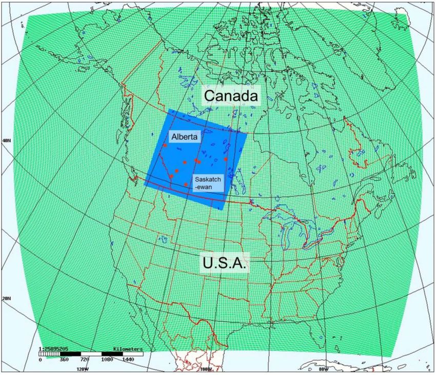
Figure 1. GEM-MACH domains. Green region: outer North Ameri- the samples were transferred from the clean collection bucket
can domain (10 km × 10 km grid-cell resolution). Blue region: inner to a smaller sample bottle, capped, refrigerated if stored on
Alberta and Saskatchewan domain (2.5 km × 2.5 km grid-cell res- site, and shipped to the laboratory for analysis. Collection oc-
olution). Red diamonds: locations of Canadian Acid Precipitation curred approximately daily at the SK sites and approximately
Monitoring Network (CAPMoN) stations used in this work.
weekly at the AB sites. Quality control was performed by the
collecting networks.
Annual precipitation-weighted mean concentrations of
ous time record of concentrations and deposition on the high- SO2− − +
4 , NO3 , and NH4 were calculated from the daily or
resolution model grid. weekly samples using recommended methods and complete-
Three simulations were carried out with this setup. The ness criteria (WMO/GAW, 2004, 2015) and the resulting de-
first of these made use of the two aerosol bin configuration position fluxes were compared with model values. Where
of GEM-MACH, for an entire year of simulated chemistry there were measurement gaps of > 3 weeks (two sites), or
and meteorology (1 August 2013 to 31 July 2014), in order where there was only partial coverage of the 12 months (one
to obtain a year of model output, required for critical load site), fluxes were compared over shorter measurement peri-
calculations. The outer 10 km North American domain of the ods. The collector buckets described above tend to underes-
simulation made use of the operational GEM-MACH fore- timate the total precipitation, so the flux of ions derived from
cast emissions inventories for the years 2010 (Canada), 2011 their records must be corrected using independent observa-
(USA) and 1999 (Mexico), while the inner nest made use of tions of total precipitation. At the SK sites, separate on-site
2013 (Canada) and 2011 (USA) inventories (see Zhang et al., rain and snow gauges were used to manually record the daily
2017). The predicted deposition thus represents the model precipitation amount. At the AB sites, precipitation gauges
predictions using emissions reported under current Canadian for independent quantification of total precipitation were not
regulatory requirements. Two additional simulations were available, and hence weekly deposition fluxes were calcu-
then carried out, for the period 13 August to 10 Septem- lated using daily precipitation depth data from the nearest
ber, making use of the 12-bin version of the model: a base meteorological station, or combination of meteorological sta-
case and a primary particulate scenario. The primary particu- tions, with the most complete coverage (ECCC, 2017; AAF,
late scenario made use of aircraft-based estimates of primary 2017).
particulate emissions from six oil sands facilities, and both Total precipitation depth collected in the AB wet depo-
making use of continuous emissions monitoring data for Al- sition collectors, summed over all collection periods at the
berta for SO2 and NOx emissions from large stack sources sites, was 51–96 % of the estimated precipitation depth at
(see Zhang et al., 2017, this issue, for the full description of meteorological stations. Our deposition flux calculations im-
these emissions). This second pair of simulations was car- plicitly assume that the ion concentrations measured in the
ried out to investigate the potential impact of possible under- sample are representative of all the precipitation during the
reporting of primary particulate emissions on model critical period. However, the mechanism of precipitation loss (un-
load exceedance predictions. About 96 % of these primary dercatch due to wind, evaporative loss, delay in lid open-
particulate emissions by mass are associated with fugitive ing) may lead to unrepresentative concentration values. Ad-
dust emissions sources, and over 68 % of this mass is in the ditional uncertainty is introduced by the use of precipitation
coarse mode (diameters greater than 2.5 µm) (Zhang et al., depth from collectors that are not co-located, particularly at
Atmos. Chem. Phys., 18, 9897–9927, 2018 www.atmos-chem-phys.net/18/9897/2018/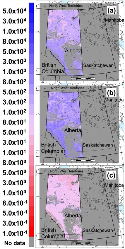
P. A. Makar et al.: Critical load exceedances for Alberta and Saskatchewan                                                 9903

Kananaskis. Therefore, wet deposition fluxes from the AB          2.3.1   Critical loads and critical load exceedances –
sites have higher uncertainty than the fluxes at the two SK               definitions
sites, where 105 and 78 % of the standard gauge precipita-
tion was captured by the collector.                               Critical loads were estimated following methodologies set
                                                                  out under the UNECE Convention on Long-range Trans-
2.2.2    Deposition of S and N compounds to snowpack              boundary Air Pollution (CLRTAP, 2017; de Vries et al.,
                                                                  2015). We define first the equations used for determining
Observations of total deposition of sulfur, nitrogen, and base    critical loads, and follow with the description of the data
cations to snow-covered open surfaces were collected in two       used to estimate critical loads of acidifying sulfur (S) and
separate studies. Samples were collected in the immediate         nitrogen (N) for terrestrial and aquatic ecosystems in Alberta
vicinity of the oil sands by Environment and Climate Change       and Saskatchewan, based on a Canada-wide implementation
Canada, and snowpack samples in northern Saskatchewan             (Carou et al., 2008), and two more recent studies focused on
were collected by Saskatchewan Environment (snowpack              terrestrial ecosystems in the province of Alberta, and aquatic
station locations are discussed in Sect. 3.4). Both sets of       ecosystems in northern Alberta and Saskatchewan (Cathcart
data were collected in open clearings and thus deposition         et al., 2016).
is to snow-covered open surfaces. They thus provide min-             For terrestrial ecosystems, critical loads of acidity were
imum estimates of deposition, particularly for gases. One         estimated using the steady-state (or simple) mass balance
method of accounting for deposition to forests and related        (SSMB) model which links deposition to a chemical vari-
vegetation is via collection of precipitation samples below       able (the “chemical criterion”) in the soil, or soil solution,
foliage, which assumes that deposited materials leave the         associated with ecosystem effects (Sverdrup and DeVries,
vegetation via precipitation and/or melting of snow, to reach     1994). The violation of a specific value (the “critical limit”)
the collector (“throughfall”). Watmough et al. (2014) com-        for the chemical criterion is associated with potential ecosys-
pared winter throughfall versus open deposition in the oil        tem damage. The most widely used soil chemical criterion is
sands region, and showed maximum throughfall values to be         based on the molar ratio of base cations to aluminum (BC : Al
about 1.9 times their open deposition counterparts. However,      where BC is the molar sum of calcium (Ca2+ ), magnesium
throughfall observations do not account for the portion of        (Mg2+ ) and potassium (K+ )) in soil solution (the factor of
the deposited material which remains on or within the veg-        3/2 in Eq. 4 below converts this term to equivalents). The
etated surfaces, and hence must also be considered a con-         acidifying impact of S and N define a critical load func-
servative estimate of total deposition. Using the algorithms      tion (CLF) incorporating the most important biogeochemi-
of GEM-MACH’s gas-phase deposition module, typical ra-            cal processes that affect long-term soil acidification (CLR-
tios of dry deposition velocity between a needle-leaf forest      TAP, 2017). The function is defined by three quantities (see
and an open snow-covered surface for SO2 and NH3 , respec-        Eqs. 1 to 4): the maximum critical load of S (CLmax (S)); min-
tively, are 2.63 and 1.97 (temperature −5 ◦ C, u∗ = 0.1 m s−1 ,   imum critical load of N (CLmin (N)); and the maximum crit-
solar radiation = 100 W m−2 , z0 = 0.1 m, Monin–Obukhov           ical load of N (CLmax (N)). The critical level of the leaching
length = 50). However, the ratios for dry deposition of par-      of acid neutralizing capacity for the ecosystem (ANCle,crit )
ticles with diameters of 2.5 and 10 µm are 0.76 and 0.82,         is defined via Eq. (4). Critical loads of acidity for terres-
respectively (Zhang et al., 2001), indicating that the open       trial ecosystems are defined in units of “equivalents” (ionic
snowpack observations may slightly overestimate BCdep and         charge × moles).
BCdep (in contrast to the Watmough et al., 2014, observa-
tions) but significantly underestimate Sdep and Ndep .            CLmax (S) = BCdep + BCw − Cldep − BCu − ANCle,crit         (1)
   Further details on the methodology used for snowpack                                   CLmax (S)
analysis may be found in the Supplement for this paper.           CLmax (N) = CLmin (N) +                                    (2)
                                                                                           1 − fde
2.3     Estimates of critical loads of acidic deposition in       CLmin (N) = Ni + Nu                                        (3)
        Canada – a review of recent work                                                                    1
                                                                                   2 3  BCw + BCdep − BCu       3
                                                                  ANCle,crit = −Q 3
In this section, we review recent work on the estimation of                          2   (BC : Al)crit Kgibb

critical loads in Canada, starting from the UNECE defini-                        3 BCw + BCdep − BCu
                                                                               −                                             (4)
tions, in order to provide a complete description of the crit-                   2      (BC : Al)crit
ical load datasets used in our subsequent estimates of ex-
ceedances.                                                          The remaining terms in these equations include BCdep , the
                                                                  non-marine annual base cation deposition, BCw , the release
                                                                  of soil base cations owing to physical and chemical break-
                                                                  down (weathering) of rock and soil minerals, CLdep , the non-
                                                                  marine chloride deposition, BCu , the average base cation
                                                                  removal due to the harvesting of base-cation-containing

www.atmos-chem-phys.net/18/9897/2018/                                              Atmos. Chem. Phys., 18, 9897–9927, 2018
9904                                             P. A. Makar et al.: Critical load exceedances for Alberta and Saskatchewan

biomass from the ecosystem, fde , the denitrification fraction      which follows), and Aj /A is the relative area of the compo-
(loss of nitrogen to N2 ), Ni , the long-term annual net immo-      nents (Aj ) to the total catchment area (A):
bilization of nitrogen in the rooting zone, and Nu , the average
                                                                                m                     m
removal of nitrogen from an ecosystem due to e.g. harvest-                      X Aj                  X Aj
                                                                    (1 − ρS )              Sdep,j +              1 − fde,j
ing); Q, defined above, (BC : Al)crit , is the critical value of                       A                     A
                                                                                j =0                  j =0
the non-sodium base cation to aluminum ion ratio described
above, and Kgibb is the Gibbsite equilibrium constant.                       Ndep,j 1 − fu,j − Ni,j − Nu,o,j + =
   For aquatic ecosystems, two steady-state models have
                                                                               "                                          #
                                                                                             m
                                                                             X             X    Aj
been widely used for calculating critical loads (Henriksen                       (1 − ρY )         Ydep,j − Yw,j − Yu,j +
                                                                                                A
and Posch, 2001; CLRTAP, 2017; de Vries et al., 2015): the                   Y             j =0
Steady-State Water Chemistry (SSWC) model and the First-                        − Q · ANClimit ,                                 (8)
order Acidity Balance (FAB) model.
   The SSWC model requires volume-weighted mean annual              where the “+” subscript refers to the maximum value of the
water chemistry and runoff volume (Q) to calculate critical         term within the brackets across the catchment components j
loads of S acidity.                                                 (lake and non-lake). Sdep includes all forms of sulfur deposi-
                                                                    tion (gaseous SO2 dry deposition, particulate dry deposition,
CL (A) = Q [BC]∗0 − ANClimit ,

                                                              (5)   and wet deposition of bisulfate and sulfate ions), converted to
                                                                    charge × mole equivalent deposition of SO2−   4 . Ndep includes
where [BC]∗0 is the sea salt corrected pre-acidification con-
                                                                    all forms of nitrogen deposition (gas-phase dry deposition of
centration of base cations in the surface water, and ANClimit
                                                                    NO, NO2 , NH3 , HONO, HNO3 , peroxyacetylnitrate, organic
is the ANC (concentration) limit above which no damage to
                                                                    nitrates, dry deposition of particulate nitrate and ammonium,
the specified biological indicator (e.g. fish) occurs. The sea
                                                                    and wet deposition of ammonium and nitrate ions), converted
salt correction, denoted by a superscript asterisk, assumes all
                                                                    to the charge × mole equivalent deposition of NO−     3 . Setting
chloride originates from sea salt; the current concentrations
                                                                    Ndep = 0 in Eq. (8) results in a formula for CLmax (S), and
of base cations, SO2−                −
                      4 (aq) and NO3 (aq) in water along with       setting Sdep = 0 results in a formula for CLmax (N). The den-
empirical functions (see below), are used to estimate [BC]∗0 ,
                                                                    itrification fraction was estimated as fde = 0.1 + 0.7 · fpeat ,
following CLRTA methodologies (CLRTAP, 2017); further
                                                                    where fpeat is the fraction of wetlands in the terrestrial catch-
details regarding the sensitivity of the critical load estimates
                                                                    ment, CLmin (N) was taken to be Ni + Nu (Ni was set to the
to these functions are described in Cathcart et al. (2016).
                                                                    regional default value of 35.7 eq ha−1 ), and Nu was based
   The FAB model (Posch et al., 2012) allows the simulta-
                                                                    on estimates of forest biomass (Canadian Forestry Service
neous calculation of critical loads of acidifying S and N de-
                                                                    National Forest Inventory) and literature data for the con-
position similar to the SSMB model widely used for forest
                                                                    centration of N in biomass. The net uptake of N on land
soil critical loads. In addition to processes in the terrestrial
                                                                    was assumed to be constant (fu,1 =0), and the flux of base
catchment soils, such as uptake, immobilization, and denitri-
                                                                    cations (right-hand side of Eq. 8) is determined using the
fication, the FAB model includes in-lake retention of N and
                                                                    SSWC model via Eq. (5). In both the SSWC and FAB mod-
S. The derivation of the FAB model starts from the charge
                                                                    els, the value of [BC]∗0 is derived using an “F -factor” equa-
balance at the outlet of a lake:
                                                                    tion describing the change in charge balance over time from
Srunoff + Nrunoff =Carunoff + Mgrunoff + Krunoff + Narunoff         pre-industrial (time 0) to current (time t) conditions:
                    − Clrunoff − ANClimit .                   (6)   [BC]∗0 =[BC]∗t − F
                                                                                · [SO4 ]∗t + [NO3 ]t − [SO4 ]0 − [NO3 ]0 .

   Steady-state mass balance equations for the runoff terms                                                                      (9)
for each ion (X) are then derived as a function of the total
                                                                       The F -factor in Eq. (9) depends on the pre-industrial base
number of ions entering the lake (Xin ) and dimensionless re-
                                                                    cation concentration and Eq. (12) is solved iteratively. The
tention factors (ρX ):
                                                                    in-lake retention coefficients for S and N (ρS and ρN , respec-
Xrunoff = (1 − ρX ) Xin .                                     (7)   tively) are modelled by a kinetic equation (Kelly et al., 1987)
                                                                    making them a function of runoff, the lake : catchment ratio,
   The formula for Xin depends on the specific ion; Sin de-         and net mass transfer coefficients for S and N. It is assumed
pends on deposition alone, Nin includes terms for net immo-         that the lakes and their catchments are small enough to be
bilization (subscript i), growth uptake (subscript u), and den-     properly characterized by average soil and lake-water prop-
itrification (fde ), and base cations include terms for deposi-     erties; furthermore, all of the lakes examined here are treated
tion (subscript dep) and weathering (subscript w). An equa-         as headwater lakes, and larger lakes are excluded from the
tion of the following form results (the summation is over the       analysis.
different components within the catchment, usually simpli-             The risk of negative impacts owing to acidifying S and N
fied to be “lake” and “non-lake”, i.e. m = 1 in the equation        deposition, i.e. deposition in excess of the critical load, is

Atmos. Chem. Phys., 18, 9897–9927, 2018                                                    www.atmos-chem-phys.net/18/9897/2018/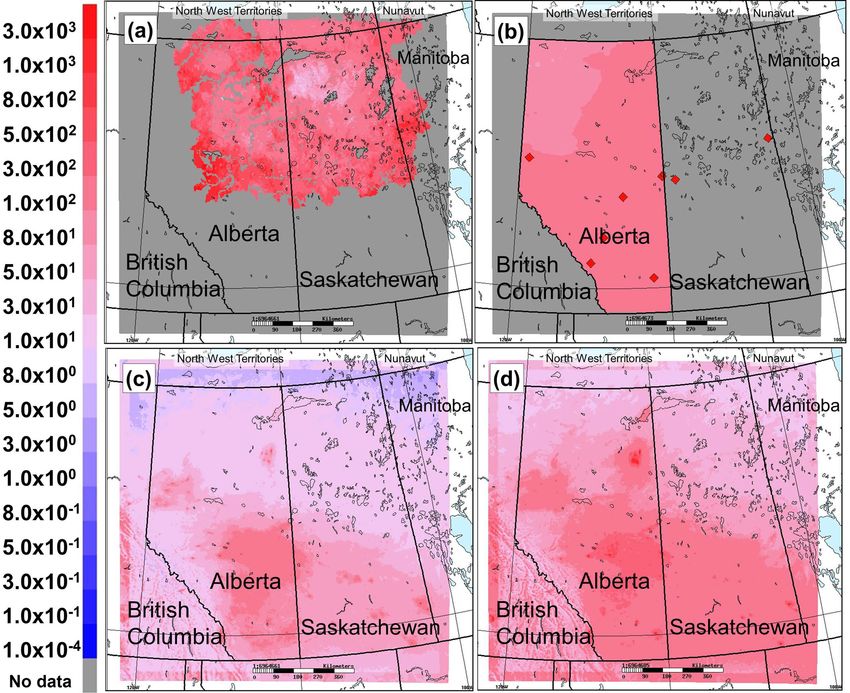
P. A. Makar et al.: Critical load exceedances for Alberta and Saskatchewan 9905
(CLmin (N), CLmax (S)) and (CLmax (N), 0), defined via
Ndep + mSdep + m2 CLmax (N)
N0 = , (12)
1 + m2
S0 = m (N0 − CLmax (N)) , (13)
where
CLmax (S)
m= . (14)
CLmin (N) − CLmax (N)
We define here E0 , a negative quantity defining the small-
est decrease in deposition from the critical load function (i.e.
the boundary between the exceedance and non-exceedance
regions of Fig. 2) to reach the Ndep , Sdep point in Fig. 2.
Sdep − CLmax (S) for Ndep ≤ CLmin (N)
Figure 2. Critical load function, showing exceedance Regions 1 E0 = Sdep − mNdep − CLmax (N) for CLmin (N) < Ndep
< CLmax (N)
through 4 and the “below exceedance” Region 0.
(15)
based on the magnitude and areal extent of exceedance. Ex- For deposition levels below exceedance, i.e. within the
ceedance of the critical load of S acidity for aquatic ecosys- grey region of Fig. 2, the value of E0 describes the proximity
tems under the SSWC model is defined as to exceedance; the fastest path by which exceedance could
occur, relative to current deposition levels. Given that Eq. (2)
Ex Sdep = Sdep − CL(A), (10) guarantees that the slope of the line joining (CLmin (N),
CLmax (S)) and (CLmax (N), 0) will always have an inclina-
where Sdep is the sum of deposition of all forms of S, where tion of less than 45◦ , the shortest path to exceedance will
each mole of S is treated as SO2− always be via the Sdep path. E0 is of potential interest to
4 (i.e. two equivalents per
mole of S deposited). Exceedances of acidity are defined as policymakers, in that this term describes the proximity of
instances where the addition of acidity in the form of S ex- regions which are not yet in exceedance of critical loads
ceeds the net buffering capacity. In contrast, under the SSMB to exceedance. Small magnitude values of E0 thus describe
and FAB models there is no unique amount of S and N to ecosystems for which small increases in Sdep or Ndep may
be reduced to reach non-exceedance; Exceedance for a given result in exceedances of critical loads. We also note that
S and N deposition pair is the sum of the S and N depo- Eqs. (11)–(14) themselves are a slight simplification for the
sition reductions required to reach the critical load function FAB model, which allows for a slight inclination of the CLF
(CLF) by the “shortest” path (Fig. 2). The computation of the for Ndep < CLmin (N).
exceedance function followed the methodology described in Three different sources of critical load data were used
CLRTAP (2017). in this work. We begin with Canada-wide critical loads of
Region 0 in Fig. 2 denotes cases for which Sdep and Ndep acidity, which employ modifications to the above UNECE
to an ecosystem are below exceedance levels (i.e. deposition methodology (CLRTAP, 2017), used in eastern North Amer-
does not exceed critical load). For this region, we introduce ica (NEG-ECP, 2001; Ouimet, 2005), and then expanded
a term E0 , a negative number indicating the proximity of de- across Canada (Carou et al., 2008; Jeffries et al., 2010; Ah-
position in Region 0 to the nearest bordering exceedance re- erne and Posch, 2013). We follow with more recent estimated
gion. Exceedances are calculated as follows. critical loads determined using the UNECE methodologies,
for terrestrial ecosystems for the province of Alberta (Aklilu
Ex Ndep , Sdep = et al., 2018), and aquatic ecosystems in northern Alberta and
Saskatchewan (Cathcart et al., 2016).
E0 Sdep , Ndep ∈ Region 0
N dep − CLmax (N) + Sdep Sdep , Ndep ∈ Region 1
2.3.2 Canada-wide critical loads of acidity: lakes and
Ndep − N0 + Sdep − S0 Sdep , Ndep ∈ Region 2
forest soils
Ndep − CLmin (N) + Sdep
−CLmax (S) Sdep , Ndep ∈ Region 3 The earliest critical load data used in the current work are
Sdep − CLmax (S) Sdep , Ndep ∈ Region 4 for forest and lake ecosystems, and resulted from updates
(11) to Environment and Climate Change Canada databases, sub-
sequent to the publication of the Canadian Acid Deposi-
For Region 2, the exceedance is defined with respect to tion Science Assessment (ECCC, 2004; Jeffries and Ouimet,
the closest point between the diagonal line joining the points 2005).
www.atmos-chem-phys.net/18/9897/2018/ Atmos. Chem. Phys., 18, 9897–9927, 2018
9906                                              P. A. Makar et al.: Critical load exceedances for Alberta and Saskatchewan

   Lake chemistry surveys were conducted in Canada in or-             plus dry) atmospheric base cation deposition data during
der to obtain data for critical load estimates (Jeffries et al.,      the period 1994–1998 were estimated using observed wet
2010). Critical loads of acidity for each sampled lake were           deposition, observed air concentrations, and modelled me-
estimated using the SSWC model (Henriksen and Posch,                  teorological data along with land-use-specific dry deposi-
2001). In addition to the lake survey data, other inputs to the       tion velocities, and mapped on the Global Environmental
SSWC include ecosystem-specific characteristics that were             Multiscale (GEM) grid at a resolution of 35 km × 35 km
estimated using a mixture of methods, including broad min-            (see Sect. 2.1 for details on GEM and its companion on-
eralogical, geological, hydrological, and biological surveys.         line chemistry module, GEM-MACH). Under the NEG-ECP
At the time these aquatic critical load data were collected,          methodology, weathering rates were estimated using a soil
acidic deposition estimates at ECCC were created using A              type-texture approximation method (Ouimet, 2005). The ap-
Unified Regional Air-quality Modelling System (AURAMS;                proach estimates weathering rate from texture (clay content)
Gong et al., 2006). The critical load values for lakes were           and parent material class. This method was used in con-
therefore gridded to the map of Canada used by the AU-                junction with the Soil Landscapes of Canada (SLC, ver-
RAMS model, with a grid-cell resolution of 45 km × 45 km.             sion 2.1) to estimate base cation weathering rates across
The SSWC critical load values for each surveyed lake con-             western Canada. Under the NEG-ECP (2001) methodol-
tained within each AURAMS grid cell were compared –                   ogy, several simplifying assumptions and/or specified func-
when data from multiple lakes within the same grid cell were          tions and values were applied to terms in Eqs. (1) through
available, the fifth percentile of the resulting critical load val-   (4): (a) a critical BC : Al molar ratio of 10, and a Kgibb of
ues was assigned to that grid cell (for grid cells containing         3000.0 m6 mol−2 charge were used, and (b) harvesting removals
less than 20 lakes, the critical load for the most sensitive lake     were not considered; therefore, long-term net uptake Nu and
was used). The lake critical load data thus represent the most        BCu were set to zero. (c) As in Sect. 2.3.3, net N immobiliza-
sensitive lake ecosystems within the given grid cell based on         tion (Ni ) was based on a 50 cm depth rooting and assumed
the available data. We note, however, that this procedure used        to be equivalent to 0.5 kg N ha−1 yr−1 (35.7 eq ha−1 yr−1 )
in the creation of this dataset (Jeffries et al., 2010) becomes       (CLRTAP, 2017). (d) Denitrification (Nde ) was also set to
less accurate as the number of lakes per grid cell becomes            0.5 kg N ha−1 yr−1 (35.7 eq ha−1 yr−1 ) following recommen-
small, with either over- or under-estimates of local ecosystem        dations in CLRTAP (2017) and Aherne and Posch (2013) as
sensitivity. This was one of the factors leading to more recent       an upper limit for well-drained soils, (e) the deposition of Cl
updates in aquatic critical load maps for Canada, discussed in        ions was assumed to be zero, (f) the weathering release of soil
more detail in Sect. 2.3.4. The resulting 45 km resolution CL         base cations (BCw ) was assumed to be dependent on temper-
maps were subsequently re-mapped to the higher-resolution             ature, (g) BCw was assumed to be equal to 0.75 BCw , and
GEM-MACH grid used here; the centroids of those 2.5 km                (h) BCdep was assumed to be equal to 0.75 BCdep . The net
GEM-MACH grid cells falling within the AURAMS lake                    critical load functions for the forest ecosystems with these
critical load polygons were assigned the corresponding AU-            simplifications become
RAMS grid critical load values. The resulting critical loads
are shown in Fig. 3a, with red values indicating the most sen-        CL (S + N) = BCdep + BCw (T )
sitive ecosystems and blue values indicating the least sen-                            "                          !# 13
sitive ecosystems. AURAMS cells for which no lake infor-                             2   3 0.75 BCw (T ) + BCdep
                                                                                 + Q3
mation was available were assigned “null” values (shown                                  2         3 × 10⁴
in grey). These critical load data identified lake ecosystems                                               !
in north-eastern Alberta, northern Saskatchewan, and north-                        3 0.75 BCw (T ) + BCdep
                                                                                 +                             + 71.4,           (16)
western Manitoba as particularly sensitive to acidifying pre-                      2            10
cipitation.
   The forest ecosystem critical loads used here began with           with
provincial and regional surveys that were combined to form                               h
                                                                                                1       1
                                                                                                           i
                                                                                          3600 281 − 274+T
a unified Canada-wide critical load dataset (Carou et al.,            BCw (T ) = BCw e                          ,                (17)
2008). Critical load and exceedance of S and N were esti-
mated for forest soils following the methodology and guide-           where T is the temperature in degrees Celsius (NEG-ECP,
lines established by the NEG-ECP (NEG-ECP 2001; Ouimet                2001; Nasr et al., 2010; Whitfield et al., 2010; Aherne, 2011).
2005), which largely follow the UNECE methodology (CLR-                  The resulting critical load values were referenced to the
TAP, 2017). The long-term critical load was estimated us-             corresponding GIS polygons under the SLC containing that
ing the SSMB model; the key spatial datasets (or base                 soil type, resulting in a Canada-wide map of forest soil crit-
maps) or formulae required for calculating critical loads             ical loads for acidity. These polygons were superimposed
are atmospheric deposition, base cation weathering rate, and          on the map of GEM-MACH 2.5 km × 2.5 km resolution grid
a critical base cation to aluminum ratio (used to calcu-              cells. Similar to the approach for lake critical loads described
late critical alkalinity leaching). Average annual total (wet         above, the 5th percentile value from the forest critical load

Atmos. Chem. Phys., 18, 9897–9927, 2018                                                www.atmos-chem-phys.net/18/9897/2018/
P. A. Makar et al.: Critical load exceedances for Alberta and Saskatchewan 9907
polygons existing within each GEM-MACH grid cell was as-
signed to that grid cell. The forest soil critical load values on
the resulting GEM-MACH grid cell thus represent the most
sensitive forest ecosystems within that grid cell. Polygons for
which forest soils were not present were assigned “null” val-
ues. Under the NEG-ECP methodology (NEG-ECP, 2001)
critical loads were simplified deposition of sulfur and nitro-
gen, as such exceedance was defined for combined deposi-
tion:
Ex Ndep , Sdep = Sdep + Ndep − CL(S + N). (18)
We note that Eq. (18), which follows the NEG-ECP
methodology (Ouiment, 2005), may lead to potential errors
at very low values of Ndep , in that the nitrogen sinks could
potentially compensate sulfur deposition. To avoid that pos-
sibility, we have added the caveat to Eq. (16) that the right-
most term is replaced by the minimum of 71.4 eq ha−1 yr−1
and Ndep (that is, the calculated nitrogen sink will not be
used to compensate Sdep , in the event that Ndep is be-
low the sum of nitrogen immobilization and denitrification
(71.4 eq ha−1 yr−1 )). In our application of this methodology
(see Sect. 3.6.1), this additional correction was found to bring
areas which were already below exceedance further below
exceedance, but had no impact on the estimate of the size
areas over exceedance, to three significant figures.
The resulting critical load map for forest soils for the first Figure 3. Critical loads of acidity on the 2.5 km GEM-MACH
of these approaches is shown in Fig. 3b, with the same colour domain, based on a Canada-wide implementation: (a) Critical
scale as Fig. 3a. The lake ecosystems can be seen to be more load for acidity (Eq. 5) and (b) forest ecosystems (Eq. 18)
(eq ha−1 yr−1 ). Forest values were calculated using 1994–1998 in-
sensitive to acidic deposition compared to forest soil ecosys-
terpolated/extrapolated BCdep observations (diamonds show the lo-
tems (lower critical load values, red shades in Fig. 3). cation of those Canada-wide stations used to estimate BCdep , which
Later in this work, we discuss the effect of different esti- reside within the 2.5 km resolution model domain). Red regions
mates of the assumed level of atmospheric base cation de- (low numbers) on the scale have the lowest critical loads, hence are
position in the above calculations towards the resulting esti- the most sensitive to deposition. No data: (a) no lake observations
mates of critical load and critical load exceedances. were available in the given 45 km × 45 km grid cell; (b) No forest
data were available and/or the “no data” regions were not forested.
2.3.3 Province of Alberta: critical loads of acidity for
terrestrial ecosystems
The SSMB model was used to estimate CLmax (S), was calculated using the Alberta Vegetation Index dominant
CLmax (N), and CLmin (N) for terrestrial ecosystems in the forest cover database to determine type and distribution of
province of Alberta following methods recommended un- forests (ABMI, 2010), harvest information (AAF, 2015), and
der the Convention on Long-Range Transboundary Air Pol- information on nutrient uptake by forest type (Paré et al.,
lution (CLRTAP, 2017). Critical loads were not derived 2012). For unmanaged ecosystems (i.e. not harvested) BCu
for areas comprising cultivated or agricultural land, rock, was set to zero, and the removal of biomass due to grazing in
and exposed or developed soil. Our initial estimate of non- grasslands was set to 8 eq ha−1 yr−1 . The acid neutralization
marine annual base cation deposition (BCdep ) was the in- capacity leaching (ANCle,crit ) was determined using critical
terpolated/extrapolated 1994–1998 base cation database de- BC : Al ratios applied by vegetation type (a (BC : Al)crit ra-
scribed above. The release of base cations as a result of tio of 6 was used for mixed forest, shrubland, and broadleaf
chemical dissolution from the soil mineral matrix (BCw ) fol- forest, while coniferous forest and grassland made use of ra-
lowed the soil texture approximation method (Eq. 17), with tios of 2 and 40, respectively). The denitrification fraction
soil information vertically weighted to a rooting depth of (fde ) was assigned using a seven-level scale (AAFC, 2010;
50 cm to create a homogeneous soil layer for calculations. CLRTAP, 2017). fde values for “very rapid”, “well”, “mod-
Soil information for this calculation was obtained from the erately well”, “imperfectly”, “poorly”, and “very poorly”
Soils Landscape Canada version 3.2 database (AAFC, 2010). drained soil were, respectively, 0.0, 0.1, 0.2, 0.4, 0.7, and
The average base cation removal in harvested biomass (BCu ) 0.8. The long-term net immobilization of N in the 50 cm
www.atmos-chem-phys.net/18/9897/2018/ Atmos. Chem. Phys., 18, 9897–9927, 2018You can also read