Addressing biases in Arctic-boreal carbon cycling in the Community Land Model Version 5 - GMD
←
→
Page content transcription
If your browser does not render page correctly, please read the page content below
Geosci. Model Dev., 14, 3361–3382, 2021
https://doi.org/10.5194/gmd-14-3361-2021
© Author(s) 2021. This work is distributed under
the Creative Commons Attribution 4.0 License.

Addressing biases in Arctic–boreal carbon cycling in the
Community Land Model Version 5
Leah Birch1 , Christopher R. Schwalm1 , Sue Natali1 , Danica Lombardozzi2 , Gretchen Keppel-Aleks3 , Jennifer Watts1 ,
Xin Lin3 , Donatella Zona4 , Walter Oechel4 , Torsten Sachs5 , Thomas Andrew Black6 , and Brendan M. Rogers1
1 Woodwell   Climate Research Center, Falmouth, MA, USA
2 National Center for Atmospheric Research, Boulder, CO, USA
3 University of Michigan, Ann Arbor, MI, USA
4 San Diego State University, San Diego, CA, USA
5 GFZ German Research Centre for Geosciences, Potsdam, Germany
6 University of BC, Vancouver, BC, Canada

Correspondence: Leah Birch (lbirch@woodwellclimate.org, birch.leah@gmail.com) and Brendan M. Rogers
(brogers@woodwellclimate.org)

Received: 1 November 2020 – Discussion started: 14 December 2020
Revised: 5 April 2021 – Accepted: 19 April 2021 – Published: 4 June 2021

Abstract. The Arctic–boreal zone (ABZ) is experiencing              ration (TER), that are more consistent with observations. Re-
amplified warming, actively changing biogeochemical cy-             sults suggest that algorithms developed for lower latitudes
cling of vegetation and soils. The land-to-atmosphere fluxes        and more temperate environments can be inaccurate when
of CO2 in the ABZ have the potential to increase in mag-            extrapolated to the ABZ, and that many land surface models
nitude and feedback to the climate causing additional large-        may not accurately represent carbon cycling and its recent
scale warming. The ability to model and predict this vulnera-       rapid changes in high-latitude ecosystems, especially when
bility is critical to preparation for a warming world, but Earth    analyzed by individual PFTs.
system models have biases that may hinder understanding of
the rapidly changing ABZ carbon fluxes. Here we investigate
circumpolar carbon cycling represented by the Community
Land Model 5 (CLM5.0) with a focus on seasonal gross pri-           1   Introduction
mary productivity (GPP) in plant functional types (PFTs).
We benchmark model results using data from satellite re-            As the atmospheric concentration of CO2 continues to rise,
mote sensing products and eddy covariance towers. We find           the Arctic–boreal zone (ABZ) is expected to continue to
consistent biases in CLM5.0 relative to observational con-          warm more rapidly than the rest of the globe (Serreze and
straints: (1) the onset of deciduous plant productivity to be       Francis, 2006; Serreze and Barry, 2011). The impacts of
late; (2) the offset of productivity to lag and remain abnor-       this accelerated warming are manifest across all major com-
mally high for all PFTs in fall; (3) a high bias of grass, shrub,   ponents of the ABZ – the cryosphere, hydrosphere, and
and needleleaf evergreen tree productivity; and (4) an under-       biosphere (Duncan et al., 2020). The multifaceted ABZ
estimation of productivity of deciduous trees. Based on these       response to warming includes accelerated carbon cycling
biases, we focus on model development of alternate phenol-          (Jeong et al., 2018), permafrost thaw, intensification of dis-
ogy, photosynthesis schemes, and carbon allocation param-           turbance regimes (Alexander and Mack, 2016), changes in
eters at eddy covariance tower sites. Although our improve-         snow cover and ecosystem water availability (Callaghan
ments are focused on productivity, our final model recom-           et al., 2011; Biancamaria et al., 2011), and shifts in vege-
mendation results in other component CO2 fluxes, e.g., net          tation structure and composition (Beck et al., 2011; Forkel
ecosystem exchange (NEE) and terrestrial ecosystem respi-           et al., 2016; Searle and Chen, 2017). These changes in the
                                                                    whole ABZ terrestrial ecosystem structure and function have

Published by Copernicus Publications on behalf of the European Geosciences Union.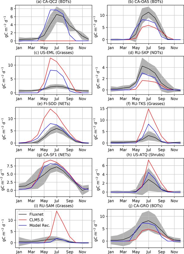
3362                                                                               L. Birch et al.: CLM5.0 biases in the ABZ

important implications for global climate, given the region’s      carbon cycling in the ABZ. In situ observations of carbon
strong biophysical coupling (Bonan et al., 1992; Bala et al.,      fluxes are required for mechanistic understanding but are of-
2007; Rogers et al., 2013, 2015) and large, and potentially        ten limited across time and space, especially in large and
vulnerable, reservoirs of below and aboveground carbon, es-        remote regions with extreme temperatures, like the ABZ
pecially in the permafrost zone (Shaver et al., 1992; McGuire      (Virkkala et al., 2018, 2019). For example, respiration dur-
et al., 2009, 2010; Koven et al., 2015; Parazoo et al., 2018b;     ing the winter has long been assumed to be effectively zero,
Natali et al., 2019; McGuire et al., 2018).                        but better technology has slowly allowed the seasonal cycle
   The responses of carbon cycling in the ABZ to changes           story to grow (Natali et al., 2019). Satellite observations pro-
in global climate are complex, interconnected, and may             vide near-complete coverage in space and time but are in-
have compensating effects (Welp et al., 2016). For exam-           direct observations of ecosystem properties, are challenging
ple, air and soil warming, in conjunction with a lengthen-         in the ABZ due to low insolation in the winter months and
ing of the annual non-frozen period across the ABZ (Kim            extreme snow storms, and contain a variety of uncertainties
et al., 2012), stimulate plant productivity directly and in-       related to sensor properties, atmospheric contamination, and
directly through increased nutrient and water availability         processing (Duncan et al., 2020). The brevity of the growing
(Natali et al., 2014; Salmon et al., 2016). Warming and            season and lack of light in the ABZ throughout the year also
CO2 fertilization have contributed to widespread “greening”        contributes to biases in satellite measurements (Randerson
across the ABZ, including shrubification (Myers-Smith et al.,      et al., 1997). Process-based models, or terrestrial biosphere
2011, 2015) and northward treeline expansion (Lloyd and            models (TBMs), are a particularly invaluable resource for
Fastie, 2003; Chapin et al., 2005), i.e., the encroachment of      examining mechanisms across spatial and temporal scales,
trees and shrubs into tundra regions. However, rapid warming       even projecting carbon cycle feedbacks in the future under
across much of the ABZ is also accelerating decomposition,         varying socioeconomic scenarios (Taylor et al., 2012; Eyring
causing drought stress in warmer and drier landscapes (Car-        et al., 2016, CMIP5 and 6). However, due to different for-
roll et al., 2011; Walker and Johnstone, 2014; Walker et al.,      mulations, assumptions, mechanisms, model inputs, and pa-
2015; Carroll and Loboda, 2017) and intensifying distur-           rameterizations, TBMs display a wide range of CO2 source–
bance regimes such as wildfire and insect outbreaks (Turet-        sink dynamics in the ABZ (Fisher et al., 2014; Huntzinger
sky et al., 2011; Kasischke et al., 2010; Rogers et al., 2018;     et al., 2013) and biases compared to observations (Schwalm
Hanes et al., 2019), all of which contribute to the increas-       et al., 2010; Schaefer et al., 2012). Given the criticality of
ingly observed patterns of “browning” in the ABZ (Verbyla,         the ABZ to future global carbon balance and the heterogene-
2011; Elmendorf et al., 2012; Phoenix and Bjerke, 2016).           ity of landscape responses to warming, it is a high priority
   As an emergent property of global change drivers in the         to understand and address the current biases in TBM carbon
ABZ, the seasonal cycle of CO2 exchange across the ABZ             cycling.
has been experiencing changes in timing and magnitude of               The Community Land Model version 5.0 (CLM5.0) is the
fluxes. Most critically regarding the magnitude of carbon          land component of the Community Earth System Mode ver-
fluxes, the atmospheric CO2 concentration in the ABZ has           sion 2.0 (CESM2.0, 2020). CLM is one of the most widely
been measured to be increasing between 30 %–60 % during            used land surface models and contributes to many global in-
the last 60 years (Keeling et al., 1996; Randerson et al., 1999;   tercomparisons (Zhao and Zeng, 2014; Peng et al., 2015;
Graven et al., 2013; Liptak et al., 2017; Jeong et al., 2018).     Ito et al., 2016) and future climate projections relevant for
Our current knowledge of the ABZ seasonal cycle of CO2             scientists and policymakers (Piao et al., 2013, e.g., IPCC).
suggests that much of the observed change in seasonal am-          The current state-of-the-art release of the Community Land
plitude is due to increased vegetation productivity during the     Model (Lawrence et al., 2019, CLM) incorporates several
growing season, a result of CO2 fertilization and warming          improvements to climatic fluxes and biogeochemistry rel-
(Forkel et al., 2016; Ito et al., 2016; Zhao et al., 2016). At     evant for the ABZ. A general improvement was observed
the same time, fall and winter respiration constitute a large      globally for CLM5.0 compared to past versions of the model
portion of the annual CO2 budget (Euskirchen et al., 2014;         (i.e., CLM 4.0 and 4.5). However, a high bias in photosyn-
Natali et al., 2019) and have been increasing with climate         thesis or gross primary productivity (GPP) at high latitudes
change (Belshe et al., 2012; Piao et al., 2008), making the        remains a well-documented issue (Wieder et al., 2019) in
implications for net sink–source dynamics uncertain (Ciais         CLM5.0. Thus, we explore the simulation of GPP along with
et al., 1995; McGuire et al., 2018). Hence, the current and        the net ecosystem exchange (NEE) and terrestrial ecosystem
anticipated state of carbon source–sink dynamics remains an        respiration (TER) in order to identify biases in the simulation
open question in part due to the uncertainty in the domi-          of the seasonal carbon balance.
nant mechanisms and differential responses governing car-              This study assesses the ability of CLM5.0 to accurately
bon fluxes across the ABZ.                                         represent CO2 fluxes with gridded model simulations, iden-
   Ground observations, satellite products, and process-based      tifies deficiencies in the simulation of ABZ carbon fluxes,
climate models are all used to understand interactions and         and provides a model recommendation for application in
feedbacks between changing environmental conditions and            the ABZ. We provide a step-by-step diagnosis of the ma-

Geosci. Model Dev., 14, 3361–3382, 2021                                            https://doi.org/10.5194/gmd-14-3361-2021
L. Birch et al.: CLM5.0 biases in the ABZ                                                                                    3363

jor factors contributing to biases in the simulation of the         diation, downward longwave radiation, 10 m wind speed, and
seasonal cycle of CO2 fluxes in CLM5.0. We use FLUX-                cloud cover fraction) from the Global Soil Wetness Project
COM (a gridded product based on machine learning; Jung              (GSWP3v1, http://hydro.iis.u-tokyo.ac.jp/GSWP3/, last ac-
et al., 2017, 2020) and the International Land Model Bench-         cess: 28 May 2021), which is a standard forcing dataset in the
marking Project (ILAMB; Collier et al., 2018) to assess             Land Surface, Snow and Soil Moisture Model Intercompari-
model results, and in situ data from FluxNet (https://fluxnet.      son Project (Van den Hurk et al., 2016, LS3MIP). GSWP3v1
fluxdata.org, last access: 28 May 2021) and Ameriflux (https:       has been shown to be appropriate and is the least biased forc-
//ameriflux.lbl.gov/, last access: 28 May 2021). We focus our       ing dataset for CLM5.0 simulations in the ABZ (Lawrence
development on the simulation of CO2 fluxes for each ABZ            et al., 2019). We begin a simulation of the CLM5.0 release
vegetation type in CLM5.0, representing the tundra and bo-          in 1850 and run through 2014 including default time series
real forest. We use point-based simulations at eddy covari-         inputs of CO2 , aerosol deposition, nitrogen deposition, and
ance (i.e., EC or flux) tower sites to inform the failure or suc-   land use change (Lamarque et al., 2010; Lawrence et al.,
cess of each model development test of the phenology and            2016), which are available on NCAR’s Cheyenne system
photosynthesis modules in CLM5.0. We validate model de-             (Computational and Information Systems Laboratory, 2017).
velopment using gridded products and additional flux towers         We implement a regional simulation of CLM5.0 north of
(withheld from the initial model development) before mak-           40◦ N across both hemispheres, allowing us to focus ex-
ing our final model recommendation. As a result, we iden-           clusively on ABZ processes. We confirm the improvements
tify and resolve many of the known biases in the representa-        made to the newly updated CLM version 5.0 (Lawrence
tion of phenology (Richardson et al., 2012), photosynthesis         et al., 2019) through a comparison of CLM version 4.5 with
(Lawrence et al., 2019), and carbon allocation in CLM5.0,           the same input datasets.
allowing a more realistic representation of carbon cycling in          For our control CLM5.0 simulation, we use an available
this rapidly changing ecosystem.                                    equilibrated 1850 initialization on NCAR’s Cheyenne system
                                                                    (Computational and Information Systems Laboratory, 2017)
                                                                    with spun-up carbon pools. After model development, we
2     Methods                                                       again spin the model using this initial dataset, and we find
                                                                    GPP to equilibrate quickly, within 20 years (Fig. S1 in the
We investigate the seasonal cycle of ABZ CO2 fluxes with            Supplement). To be conservative, we spin up the model with
CLM5.0 due to its widespread use and significant model im-          our recommended model development versions for 100 years
provements from the previous version. These updated pro-            to ensure carbon fluxes have come to equilibrium. Then we
cesses include snow physics related to snow age and den-            use this equilibrated state as initial conditions in a produc-
sity, canopy snow interactions, active layer depth, groundwa-       tion simulation beginning in 1850 with all the same configu-
ter movement, soil hydrology and biogeochemistry, and river         rations and climatology as the CLM5.0 release control simu-
transport (Li et al., 2013). Moving away from globally con-         lation.
stant values of plant traits that are challenging to measure,          Typical of land surface models, CLM5.0 represents vege-
carbon and nitrogen cycle representations now use prognos-          tation through broad plant functional types (PFTs). CLM5.0
tic leaf photosynthesis traits (the maximum rate of electron        represents ABZ vegetation using five PFTs: needleleaf ever-
transport or Jmax and the maximum rate of carboxylation or          green boreal trees (NETs), needleleaf deciduous boreal trees
Vcmax ; Ali et al., 2016), carbon costs for nitrogen uptake, leaf   (NDTs), broadleaf deciduous boreal trees (BDTs), decidu-
nitrogen optimization, and flexible leaf stoichiometry. Stom-       ous boreal shrubs (hereafter “shrubs”), and arctic C3 grasses
atal physiology was updated with the Medlyn conductance             (hereafter “grasses”). We focus model development on PFT-
model, replacing the Ball–Berry model (Medlyn et al., 2011).        specific comparisons, which allows a direct comparison with
Additionally plant hydraulics have recently undergone im-           observational data. Any improvements to PFT-specific car-
provement in more realistic stress representation (Kennedy          bon flux simulations have implications for changing vegeta-
et al., 2019). One primary goal with these improvements was         tion distributions in the ABZ.
to allow for more physically based parameters that could be
informed by observational ecological data, ultimately allow-        2.2   Model benchmarking and validation with
ing for better fidelity with hydrological and ecological pro-             FLUXCOM and ILAMB
cesses. Land cover inputs to CLM5.0 were updated to capture
transient land use changes from the satellite record.               Benchmarking is the process of quantifying model perfor-
                                                                    mance based on observational data considered to be the ex-
2.1    Pan-Arctic CLM5.0 simulation                                 pected value or truth. We use FLUXCOM (Tramontana et al.,
                                                                    2016; Jung et al., 2017, 2020) to benchmark gridded CO2
We run CLM5.0 at 0.5◦ by 0.5◦ grid resolution with mete-            fluxes (i.e., gross primary productivity, terrestrial ecosystem
orology inputs (rainfall, snowfall, 2 m air temperature, 2 m        respiration, and net ecosystem exchange, or GPP, TER, and
specific humidity, surface pressure, downward shortwave ra-         NEE) in CLM5.0. FLUXCOM is an upscaled machine learn-

https://doi.org/10.5194/gmd-14-3361-2021                                              Geosci. Model Dev., 14, 3361–3382, 2021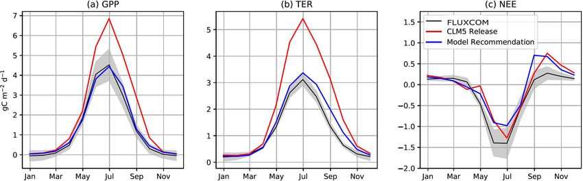
3364                                                                                L. Birch et al.: CLM5.0 biases in the ABZ

ing product based on FLUXNET eddy covariance towers.                sonal CO2 fluxes, which is a standard model development
As a global product, FLUXCOM is particularly useful for             procedure (Stöckli et al., 2008a). We aggregate fluxes of CO2
filling spatial gaps in tower observations, especially in the       to monthly means from flux towers in the ABZ that are part
relatively data-sparse ABZ. This product uses multiple re-          of the FluxNet (https://fluxnet.fluxdata.org, last access: 28
analysis datasets and machine learning methods to train mul-        May 2021) and Ameriflux (https://ameriflux.lbl.gov/, last ac-
tiple predictors at flux tower sites. The resulting product is      cess: 28 May 2021) networks. We screen the tower records
the mean of those ensembles, which also allows standard er-         to determine whether the PFT type in CLM5.0 corresponds
ror to be calculated. We use the standard deviation around          to the vegetation described by tower metadata. We choose
the mean to identify successful model development. Machine          towers and grid cells with at least 3 years of sample data
learning is a useful tool for this type of gap filling, as it       before 2014, as that is the end date of GSWP forcing data
does not care about geographic locations, just the predictor        for CLM5.0. Collectively, the chosen towers that conform to
space, which are the fluxes and environmental conditions.           our data requirements span all PFT types over the ABZ (Ta-
FLUXCOM is unable to simulate fluxes from fires and CO2             ble S1 in the Supplement). We divide our observational data
fertilization accurately, which is why we focus model de-           into model development sites vs. evaluation sites to prevent
velopment on averages over the past couple decades, rather          overfitting of parameters. Our chosen model development
than specific years with forest fires and the increasing CO2        sites are US-EML (Belshe et al., 2012), CA-QC2 (Margolis,
amplitude trend. Any systemic problems with FLUXNET                 2018), CA-OAS (Black, 2016, BDT), and RU-SKP (Maxi-
data would also exist within FLUXCOM, but validations of            mov, 2016), which encompass all of the CLM5.0 PFTs. We
regions with sun-induced chlorophyll fluorescence (Köhler           verify our work using additional flux tower measurements
et al., 2015, SIF) add confidence in the FLUXCOM product.           from FI-SOD (Aurela et al., 2016), RU-Tks (Aurela, 2016),
Additionally, derived from global MODIS-based vegetation            CA-Sf1 (Amiro, 2016), US-Atq (Oechel et al., 2014), RU-
layers Sulla-Menashe and Friedl (2019), FLUXCOM has the             Sam (Kutzbach et al., 2002–2014; Holl et al., 2019; Runkle
ability to generate PFT-specific output. Although there are         et al., 2013), and CA-Gro (McCaughey, 2016).
inconsistencies between the PFT classifications, such as the            During our model development process, we examine phe-
representation of “mixed forests” in FLUXCOM, this allows           nology and photosynthesis schemes in CLM5.0 by running
direct comparisons of the PFT-specific fluxes represented by        point simulations starting in 1901 using the same inputs
CLM5.0.                                                             as our gridded simulations. For each model issue listed in
    For an independent set of comparisons that includes addi-       Sect. 2.4, we iteratively test hypotheses and ranges of param-
tional environmental variables, we also use the International       eters values that may improve the simulation at the represen-
Land Model Benchmarking System (Collier et al., 2018, IL-           tative towers. Point simulations allow for rapid deployment
AMB). ILAMB is an open-source land model evaluation sys-            of model tests, while also conserving computing resources.
tem that provides a uniform approach to benchmarking and            This speed of computation is invaluable for our multiple
scoring model fidelity. It is a powerful tool to quickly and        model development trajectories. We find that for our focus
thoroughly investigate biases, seasonality, spatial distribu-       on phenology and photosynthesis, carbon fluxes equilibrate
tion, and interannual variability in climate model output. We       rapidly and a 20-year spin-up is sufficient for point simula-
use ILAMB to benchmark fluxes of CO2 , moisture, and heat,          tions (Fig. S1 in the Supplement). We run the point simula-
in addition to several land surface properties essential for cli-   tions through 2014 and compared the years measured by flux
mate responses and feedbacks such as albedo and leaf area           towers with the same years simulated by CLM5.0. We ac-
index (LAI). Although the focus of our model development is         knowledge that the climatology experienced by a given flux
on GPP, TER and NEE tend to respond strongly to changes in          tower and the reanalysis data used as model input are differ-
productivity (Chapin et al., 2006; Schaefer et al., 2012; Chen      ent. Thus, we focus on the mean seasonal behavior of the flux
et al., 2015). We benchmark these additional interdependent         towers and CLM5.0 to guide model development. The yearly
properties in ILAMB to ensure our development generates             variance serves as an uncertainty range for our characteri-
systematic improvements.                                            zation of flux tower behavior. Additionally, using the mean
                                                                    monthly CO2 fluxes as calibration data can prevent over-
2.3    Point simulation protocol                                    fitting of CLM5.0 parameters. Each model development sim-
                                                                    ulation for a specific PFT is also run for the other PFTs at the
Although FLUXCOM is an invaluable tool to fill spatial              development sites (CA-QC2, CA-OAS, US-EML, and RU-
and temporal gaps in tower observations across the ABZ,             SKP). After finalizing a given model development scheme,
it is by definition not as accurate as direct in situ obser-        we implement the updates at the withheld EC sites (Table S1
vations of CO2 fluxes, for instance measurements from EC            in the Supplement) and then in a gridded fashion across our
towers, which also include helpful ancillary information            ABZ regional domain.
such as detailed vegetation composition. After benchmark-
ing the aggregated grid cell fluxes, we assess model perfor-
mance at specific EC towers that measure year-round sea-

Geosci. Model Dev., 14, 3361–3382, 2021                                             https://doi.org/10.5194/gmd-14-3361-2021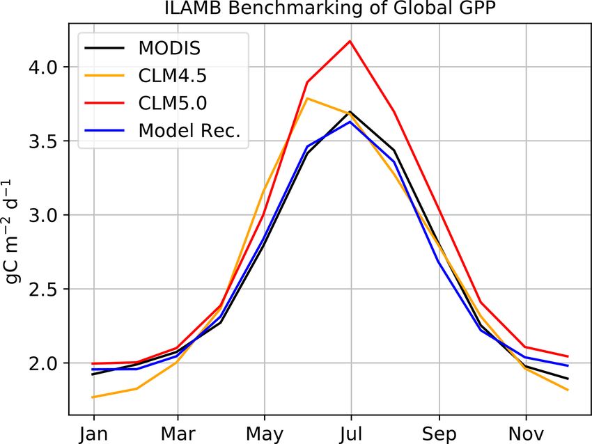
L. Birch et al.: CLM5.0 biases in the ABZ                                                                                   3365

2.4     Model development                                            For our ABZ deciduous phenology algorithm, we there-
                                                                  fore allow photosynthesis to begin when the following envi-
We identify several issues in the phenology and photosyn-         ronmental criteria occur:
thesis schemes in CLM5.0 for the ABZ, which are detailed
in Sect. 3.1. These can be categorized by (i) extrapolation of     1. The 10 d average soil temperature in the third soil layer
schemes and parameterizations designed for temperate veg-             is above 0 ◦ C.
etation, (ii) biases in the prediction of leaf photosynthetic
                                                                   2. The 5 d average minimum daily 2 m temperature aver-
traits, and (iii) mis-specified carbon allocation parameters.
                                                                      age is above 0 ◦ C.
We also incorporate a bug fix as detailed in Sect. S3 in the
Supplement.                                                        3. Only a thin layer of snow remains on the ground (<
                                                                      10 cm).
2.4.1    Phenology onset
                                                                  Together, these metrics approximate when plants begin pho-
The representation of spring and autumn phenology for de-         tosynthesis in spring, allowing for roots to absorb moisture
ciduous trees, shrubs, and grasses in CLM5.0 is based on a        in unfrozen soil, for air temperatures to be consistently above
study of the conterminous United States (White et al., 1997)      freezing, and for plants to no longer be covered in snow.
and extended to the ABZ. In the extratropics, plants initiate
their photosynthetic growing season in response to various        2.4.2   Phenology offset
climatic factors in spring, reach peak productivity in sum-
mer, and enter dormancy in autumn. This is parameterized in       Fall deciduous phenology in CLM5.0 is based on the same
CLM5.0 by allowing spring onset to begin once a threshold         study focused on the temperate latitudes (White et al., 1997).
for cumulative growing degree days is met, as determined          As with phenology onset, biases arise from the extrapolation
by White et al. (1997) using relationships between tempera-       of temperate-zone relationships to the high latitudes. Using
tures and the satellite-based normalized difference vegetation    NDVI, senescence was identified to occur in autumn when
index (NDVI). Thus, in CLM5.0, onset is based on relation-        daylight decreases ∼ 11 h. This daylight threshold is then
ships derived from temperate latitudes and extrapolated to        set to be a global constant in CLM5.0. Complete dormancy
the ABZ. We find that this parameterization requires rela-        is reached after 30 d after this photoperiod threshold. In the
tively warm temperatures for the ABZ before onset can be-         ABZ, this threshold of 11 h of total daylight generally causes
gin, which causes a delay in the beginning of the growing         plants to decrease productivity in October and to begin dor-
season for deciduous plants in the ABZ.                           mancy in November. In reality, vegetation should be reaching
   To implement a more mechanistic approach to onset in the       dormancy at the end of September in the high Arctic (Zhang
ABZ, we identify environmental thresholds that correspond         et al., 2004), with senescence beginning in August (Corradi
to physiological changes during spring onset in high lati-        et al., 2005). Based on existing physiological studies of ABZ
tudes. Field observations consistently demonstrate that pro-      vegetation, it is unclear if temperature or photoperiod are the
ductivity initiation in the ABZ is governed by the cessation      driving factor that triggers fall senescence (Marchand et al.,
of freezing temperatures (Ueyama et al., 2013; Stöckli et al.,    2004; Eitel et al., 2019), or if a combination of both is neces-
2008b) and the availability of soil water (Goulden et al.,        sary for ABZ senescence (Oberbauer et al., 2013). Therefore,
1998). Additionally snow cover has been shown to influ-           we focus on photoperiod, which is seasonally more consis-
ence the start of the growing season (Høye et al., 2007; Se-      tent across the ABZ and clearly crucial for photosynthesis.
menchuk et al., 2016). We use daily output from FLUXCOM           Based on observations at high latitudes, 15 h is a more accu-
and flux towers to identify the initiation of GPP in spring for   rate timing for senescence above 65◦ N (Corradi et al., 2005;
different PFTs. We then compare the timing of productivity        Eitel et al., 2019). We scale the photoperiod threshold lin-
to a variety of CLM5.0 environmental variables known to           early along a latitudinal gradient from 65◦ N until ∼ 11 h at
correspond strongly with GPP onset (Chapin III and Shaver,        45◦ N such that the temperate latitudes retain the offset tim-
1996; Starr and Oberbauer, 2003; Borner et al., 2008), in-        ing determined by White et al. (1997).
cluding soil temperature, soil moisture, soil ice content, air
temperature, liquid and ice precipitation, snow depth, and la-    2.4.3   Day length scaling for photosynthetic parameters
tent and sensible heat fluxes (Fig. S2 in the Supplement). We
                                                                  The Farquhar model of photosynthesis for C3 plants uses two
find that soil temperature (and thus soil ice content in the
                                                                  main parameters to represent photosynthetic capacity, Jmax
third soil layer with ∼ 10 cm depth), minimum 2 m tempera-
                                                                  (the maximum rate of photosynthetic electron transport) and
ture, and snow cover undergo notable state transitions around
                                                                  Vcmax (the maximum rate of rubisco carboxylase activity). In
the timing of GPP onset, enabling their use as a phenology
                                                                  the current release of CLM5.0, Jmax and Vcmax are predicted
threshold in CLM5.0.
                                                                  by a mechanistic model of Leaf Utilization of Nitrogen for
                                                                  Assimilation (LUNA; Ali et al., 2016). Unlike previous ver-
                                                                  sions of CLM, both Jmax and Vcmax are prognostic in CLM

https://doi.org/10.5194/gmd-14-3361-2021                                            Geosci. Model Dev., 14, 3361–3382, 2021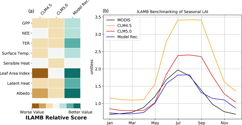
3366                                                                                   L. Birch et al.: CLM5.0 biases in the ABZ

5.0, which allows for the vegetation to adjust to nutrients and    in Kattge and Knorr (2007) we choose to implement temper-
environmental conditions. In our comparison of productivity        ature scaling functions from Leuning (2002), which does not
in CLM5.0, we find that the prediction of Jmax and Vcmax           create a discontinuity in Jmax and Vcmax at such a critical tem-
may be biased high in the ABZ (Rogers et al., 2017) when           perature for the ABZ. This is a standard implementation of
using algorithm values and schemes more appropriate for the        the Arrhenius temperature response function, which has been
tropics and temperate regions, which contributes to the over-      shown to work well at lower temperatures under present cli-
estimation of GPP by CLM5.0 across the ABZ.                        mate conditions in previous versions of CLM. The shift from
   Currently, Jmax is scaled in LUNA using day length:             Leuning (2002) to Kattge and Knorr (2007) was originally
                                                                   made due to improved process understanding of acclimation
                   daylength 2

f (daylength) =                  .                           (1)   in photosynthesis, but Kattge and Knorr (2007) would only
                       12                                          be suitable if ABZ sites had been included in the parameteri-
The function, f (daylength), is a scaling factor that is based     zation. Without those sites, it is an extrapolation of the south-
on the formulation in Bauerle et al. (2012), which quantifies      ern scheme to the ABZ, which we find introduces significant
the relationship between day length and Jmax . However, the        biases.
denominator in this equation in CLM5.0 is set to 12 h, when
                                                                   2.4.5    Jmax and Vcmax winter default
it should be the maximum day length possible at a particular
latitude (Bauerle et al., 2012). While 12 h is fairly represen-    The LUNA module calculates Jmax and Vcmax dynamically
tative for lower latitudes, this scale factor does not work for    during the growing season only. When plants are dormant
the ABZ where some regions experience up to 24 h of day-           in winter (non-growing season), CLM5.0 uses constant val-
light in summer, which allows f (daylength) > 1 in Eq. (1),        ues (see equations in the Supplement Sect. S4). Thus, at the
particularly around the summer solstice in June. To address        start of the growing season (or first day of spring), Jmax,t and
this, we replace the default denominator of 12 h with the ge-      Vcmax,t are directly calculated from a winter constant value:
ographically specific annual maximum hours of daylight that
occur for a given grid cell.                                       Jmax, last day of winter = Jmax,t−1 = 50,                    (2)
2.4.4   Temperature acclimation                                    Vcmax, last day of winter = Vcmax,t−1 = 85.                  (3)

Within both the photosynthesis and LUNA schemes in                 We find that this global default winter value strongly influ-
CLM5.0, Jmax and Vcmax are scaled from their values on the         ences the prediction of Jmax and Vcmax throughout the en-
environmental leaf temperature and to 25 ◦ C using a mod-          tire growing season (Fig. S4 in the Supplement). In all of
ified Arrhenius temperature response function from Kattge          the ABZ PFTs, raising these default values increases mean
and Knorr (2007, Fig. S3 in the Supplement). Currently, Jmax       growing-season GPP, whereas decreasing them lowers GPP
and Vcmax are allowed to acclimate to the plant’s growth tem-      (Fig. S4 in the Supplement). Furthermore, the constant win-
perature, defined as the 10 d average 2 m temperature. How-        ter values in Eq. (3) represent a high bias globally in Vcmax
ever, the temperature acclimation function is limited to tem-      (Lawrence et al., 2019), contributing additional bias. Due to
peratures between 11 and 35 ◦ C and tuned to mostly tem-           the sensitivity of this choice and in an effort to leverage the
perate species (Kattge and Knorr, 2007). At temperatures           physiological history of a given location, we choose to save
outside of the acclimation range, the temperature acclima-         the average predictions of Jmax and Vcmax from the previous
tion function scales Jmax and Vcmax to unusually high values       growing season for all PFTs (Jmax, prevyr and Vcmax, prevyr ).
(Fig. S3 in the Supplement), likely due to the use of tem-         We preserve the LUNA equations, except these constant val-
perate species for parameterization tuning. The mean daily         ues.
summer temperature in the ABZ above 60◦ N is below 11 ◦ C
(NCEP/NCAR reanalysis; Kalnay et al., 1996), which im-             Jmax, pft, last day of winter = Jmax, pft, prevyr            (4)
plies vegetation at this latitude may never enter the range        Vcmax, pft, last day of winter = Vcmax, pft, prevyr          (5)
for temperature acclimation designated by Kattge and Knorr
(2007). The temperature scaling done below 11 ◦ C is not           2.4.6    Carbon allocation
based on any ABZ studies, nor does it match the previ-
ous scaling used in CLM5.0 parameterizations from Leun-            Finally, we investigate the sensitivities of parameters re-
ing (2002), which do contain some field sites in the ABZ.          lated to carbon allocation, which are relatively uncertain and
At more southern locations in the ABZ, vegetation may fluc-        strongly influence CO2 fluxes in the ABZ, particularly the
tuate around this minimum threshold value of 11 ◦ C, allow-        stem-to-leaf ratio and the root-to-leaf ratio. In CLM5.0, the
ing discontinuities to appear in the temperature scaling of        parameter defining the root-to-leaf allocation ratio is set at
Jmax and Vcmax and influencing biases in the seasonality of        a constant value of 1.5 for all PFTs. This is not an ideal
CO2 fluxes. Due the lack of observational data across the          configuration as boreal trees and tundra vegetation are struc-
ABZ incorporated in the Arrhenius function for acclimation         turally different than other plant types due to the need to cope

Geosci. Model Dev., 14, 3361–3382, 2021                                                https://doi.org/10.5194/gmd-14-3361-2021
L. Birch et al.: CLM5.0 biases in the ABZ 3367
with colder temperatures, which should be reflected in al- as detailed in Sect. 2.2. We address the biases that arise from
location to their roots, leaves, and other plant components. using the default CLM5.0 parameters and schemes described
Even within a PFT, different species have been measured in Sect. 2.4, which can be classified as (1) phenology onset,
to have drastically different ratios of allocation to roots and (2) phenology offset, (3) daylight scaling, (4) Leuning tem-
leaves (Iversen et al., 2015), but for the purpose of circum- perature scaling, (5) initial spring value of Jmax /Vcmax , (6)
polar simulations, we limit our allocation parameters to the dynamic stem-to-leaf carbon allocation, and (7) realist root-
PFT level. Root-to-leaf ratios have been measured as consis- to-leaf carbon allocation.
tently high for grasses and shrubs, meaning more allocation
to roots than leaves (Chapin III, 1980; Iversen et al., 2015),
3.1 Biases in CLM5.0
as the large root systems are key to survival of these Arc-
tic species (Archer and Tieszen, 1983). We, therefore, tested
a higher root-to-leaf allocation of 2 for shrubs and grasses, The latest release of CLM5.0 substantially overestimates
which agrees relatively well with observations of tundra veg- summer GPP in the ABZ by ∼ 3 g C m−2 d−1 or 40 % (red
etation (Buchwal et al., 2013). For boreal trees, belowground line in Figs. 1b and 2a). The magnitude of this bias is such
allocation in evergreen conifers has been found to be higher that CLM5.0 estimates of GPP for high-latitude tundra veg-
than in deciduous trees (Gower et al., 2001; Kajimoto et al., etation are comparable with the more southern boreal forests
1999). Lowering the root-to-leaf ratio of DBT to 0.75 better (Fig. 1a). This lack of a latitudinal gradient in CLM5.0 is
represents the typically shallow root systems of deciduous not supported by FLUXCOM and ILAMB benchmarking
boreal trees (Kobak et al., 1996), while being consistent with (Fig. 1f). Though most of the ABZ in CLM5.0 is over pro-
values implemented in other deciduous tree modeling stud- ductive, we note that there is a large area with GPP = 0 in
ies (Arora and Boer, 2005). Observations suggest that boreal Siberia, indicating that this region is not photosynthesizing
NETs in general have more extensive root systems than the in CLM5.0 though it should be. Thus, the simulation of car-
deciduous trees (Gower et al., 1997), thereby requiring more bon fluxes in CLM5.0 is very heterogeneous with areas that
belowground resources, and that tundra shrubs and grasses are highly productive and areas that are non-functioning, or
allocate even more photosynthate belowground. Thus, obser- “dead zones”.
vations provide support for NET root-to-leaf allocation to be We next investigate the seasonal cycle of CO2 fluxes in the
larger than DBT, and we choose to allow the NET root-to- ABZ. Across the ABZ, average productivity in the CLM5.0
leaf allocation to remain at the CLM5.0 default value. simulation is high throughout the year compared to FLUX-
Regarding stem allocation, CLM5.0 includes an option for COM, which is shown throughout the year in Fig. 2a. From
dynamic stem-to-leaf allocation. The ratio is based on NPP a seasonal perspective, CLM5.0 vegetation enters dormancy
and can be used for woody trees and shrubs (Friedlingstein later than observations, as can be seen by the high biases in
et al., 1999), generally acting to increase woody growth in GPP in fall. The timing of photosynthesis in spring appears
favorable conditions (Vanninen and Mäkelä, 2005). Though to be accurate when we look at the PFT-aggregated average
this allocation was previously used in CLM4.5 and turned of CO2 fluxes. We see a similar high bias in TER in Fig. 2b,
off for CLM5.0, it is an uncertain choice as noted explic- as respiration is tightly coupled to the highly biased GPP. The
itly in Lawrence et al. (2019). A problem with this alloca- magnitude of peak summer NEE in CLM5.0 matches obser-
tion scheme was noted in the tropics (Negrón-Juárez et al., vational data better than GPP and TER. However, its seasonal
2015), but not in temperate or high-latitude climates. We test cycle exhibits biases and timing issues related to spring draw-
both options, comparing the static stem-to-leaf ratios used in down, summer minimum, and fall peak NEE (Fig. 2c).
CLM5.0 to the dynamic allocation option. Assessing the seasonality of CO2 fluxes in the ABZ using
the PFT-specific output of CLM5.0 reveals biases in phenol-
ogy that are hidden when PFTs are aggregated together in a
3 Results grid cell. In terms of phenology, we find that NET begins sig-
nificant photosynthesis in February in CLM5.0 when air tem-
We investigate the simulation of CO2 fluxes in the Arctic– peratures are well below freezing. This onset of NET photo-
boreal zone by CLM5.0 using gridded and point simula- synthesis is considerably early according to both FLUXCOM
tions. We identify biases in the carbon cycle in Sect. 3.1, (Fig. 3b) and our understanding of available liquid water for
present our mechanistic and additive improvements to phe- photosynthesis (Goulden et al., 1998). The peak productivity
nology and photosynthesis in Sect. 3.2, and make our model in NET occurs in June, instead of July as seen in observa-
recommendation in Sect. 3.3. This ABZ analysis focuses pri- tional data. In contrast, the onset of photosynthesis for decid-
marily on GPP fluxes in CLM5.0, but as expected, our as- uous trees and shrubs is consistently late (Fig. 3). The grid-
sessment extends to TER and NEE due to the interdepen- ded CLM5.0 GPP output hides these biases, showing that on
dence of these carbon fluxes on productivity (Chen et al., average onset in CLM5.0 matches observations (Fig. 1a). In
2015). We assess simulation biases based on the compari- contrast, the high bias of CLM5.0 productivity during late
son of CLM5.0 output against FLUXCOM and EC towers, autumn was easily seen in the gridded CLM5.0 output, and
https://doi.org/10.5194/gmd-14-3361-2021 Geosci. Model Dev., 14, 3361–3382, 20213368 L. Birch et al.: CLM5.0 biases in the ABZ Figure 1. Average summer (JJA) GPP (g C m−2 d−1 ) for (a) CLM5.0 release, (b) our model recommendation, and (c) FLUXCOM, with the differences between the two model simulations and FLUXCOM in (b) and (d). The latitudinal gradient of summer GPP is depicted in (f). Figure 2. The annual cycle of (a) GPP, (b) TER, and (c) NEE from CLM5.0 and our model recommendation compared to FLUXCOM in the ABZ. Non-productive grid cells in the ABZ are removed from the average, meaning where LAI = 0, which is standard procedure in CLM analysis (Lawrence et al., 2019). Geosci. Model Dev., 14, 3361–3382, 2021 https://doi.org/10.5194/gmd-14-3361-2021
L. Birch et al.: CLM5.0 biases in the ABZ 3369
we confirm that this bias is due to the shifted seasonal cycle 3.2 Model development at flux towers
of deciduous PFTs (Fig. 3).
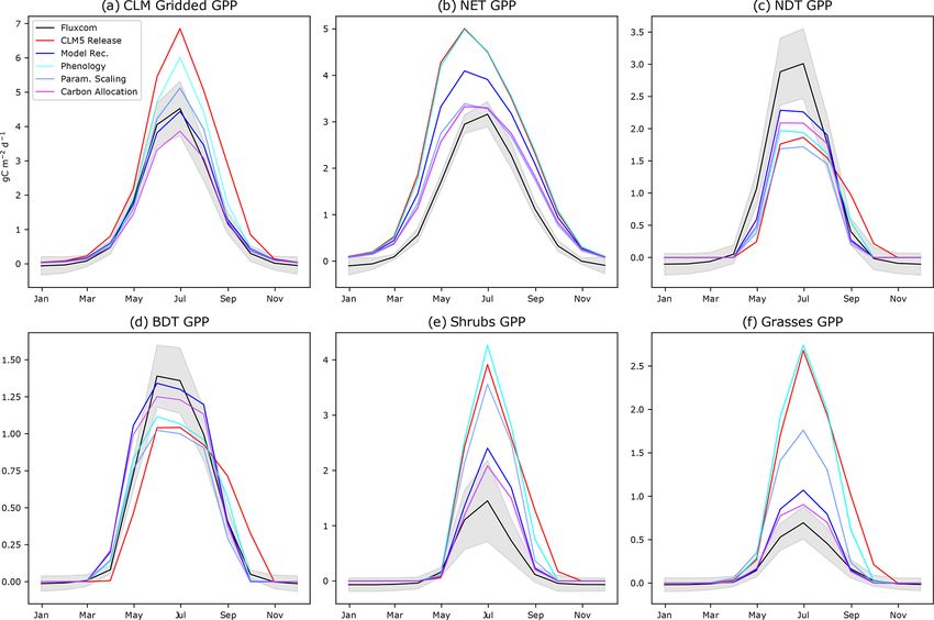
Regarding the magnitude of photosynthesis, the CLM5.0 We confirm these biases in the ABZ by comparing the
PFT-specific output indicates that both shrubs and grasses CLM5.0 PFT-specific output to representative flux towers
have a large high bias of GPP compared to observational data across the ABZ. For example, the southern boreal mixed for-
by a factor of 2–3 (Fig. 3a). We confirm that the tundra grass est site at CA-QC2 (Fig. 4a) contains NET, BDT, and shrub
and shrub PFT-specific output is often greater than or as pro- PFTs. The BDT here is a dead zone, where GPP = 0, mak-
ductive as the boreal trees in CLM5.0 (Fig. 3e and f vs. b– ing it a useful site to understand what model thresholds may
d). The deciduous boreal trees (NDT and BDT) have a low be influencing one PFT to die out in a simulation, while oth-
growing-season GPP bias, while NETs have a high produc- ers remain productive. We also include a BDT site at CA-
tivity bias. By examining the spatial pattern of the average OAS (Fig. 4b) to further investigate the simulation of decid-
summer GPP (Fig. 1), one can see that there are many ar- uous trees at a productive grid cell in CLM5.0. The grasses
eas where GPP = 0 for many consecutive years, indicating and shrubs at Eight Mile Lake, Alaska, are approximately
that the PFT did not survive. In Siberia, a prominent “dead 5 times more productive than observations (Fig. 4c). In con-
zone” occurs in what should be highly productive deciduous trast, at the larch forest at RU-SKP (Fig. 4d), we find that
needleleaf larch forests. Smaller dead zone areas are present onset is late and GPP is roughly half the observed value,
for all other PFTs across the ABZ (Fig. S5 in the Supple- consistent with the low bias in NDT gridded output. We per-
ment). form model development by examining each issue described
As with the aggregated CLM5.0 output, the PFT-specific in Sect. 2.4 sequentially on our model development sites:
biases in TER are similar to those noted for GPP (Fig. S6 CA-QC2, CA-OAS, US-EML, and RU-SKP. Each flux tower
in the Supplement). PFT-specific patterns in NEE also tend measurement is carefully chosen to cover all CLM5.0 PFTs
to follow the biases in GPP and TER, with the notable ex- to understand their complex impacts on GPP across all PFTs,
ception of spring in deciduous vegetation. For these PFTs, while also including a dead zone to tease out a different kind
there is a large spike of CO2 released to the atmosphere, up to of bias. Model development follows the procedure and bi-
0.5 g C m−2 d−1 between April and May, that does not match ases described in Sect. 2; we begin with phenology, move
observations (Fig. S7 in the Supplement). This is primarily on to the photosynthesis schemes, and end with adjusting
due to the late-onset photosynthesis at a time when TER is the carbon allocation parameters. The use of flux towers and
increasing due to warming air and soil temperatures. We note point simulations allow us to test a range of hypotheses for
that the net balance of BDTs is near 0, rather than a sink, each model development objective. Successful model devel-
which agrees with our conclusions that deciduous trees are opment is achieved when GPP is within standard deviation
not productive enough relative to FLUXCOM and flux tow- limits. We choose to make the model development additive
ers. Ultimately, the timing and magnitude of biases in TER because the improvements are generally small and justified
and NEE confirm our need to focus on GPP as a first step observationally, but all together make for a substantially im-
towards better representing seasonal CO2 fluxes in CLM5.0 proved simulation of ABZ carbon fluxes (Fig. 3).
for the ABZ. Regarding phenology, when new thermal and moisture
Benchmarking CLM5.0 yields the following primary is- thresholds for onset are used, the deciduous plants to be-
sues for the simulation of GPP across the ABZ: gin photosynthesis earlier in the season, which more closely
matches observations (Fig. 3). However, the bias in the mag-
1. The onset of GPP in deciduous PFTs in spring is con-
nitude of photosynthesis is not improved by our phenology
sistently late across all PFTs.
changes; in fact, the productivity of grasses and shrubs in-
2. The fall senescence of GPP is consistently late. creases further with a growing season that begins earlier in
spring (Fig. 3e and f, comparing the red “CLM5.0 Release”
3. There is no latitudinal gradient in summer GPP, due in line to the cyan “Phenology” line).
part to the high GPP bias in tundra grasses and shrubs. Next, regarding Jmax , we find that modifying the function
4. NETs begin photosynthesis early in winter and reach that scales Jmax to accurately use the maximum number of
their peak in productivity in June, instead of July. daylight hours on each grid cell (Bauerle et al., 2012) de-
creases productivity across all PFTs (Figs. 4 and S8 in the
5. NETs have a high GPP bias throughout the growing sea- Supplement). In particular, we decrease the June spike in
son. GPP for NET because the daylight fraction around the sum-
6. Deciduous trees (BDTs and NDTs) have a low GPP mer solstice is no longer greater than 1. Overall, this modifi-
bias. cation decreases the high bias in ABZ GPP by 2 g C m−2 d−1
in the summer (Fig. S8 in the Supplement) and generates
7. There are large areas of PFTs that have no productivity a latitudinal gradient in the PFT-specific output of trees
at all or are effectively dead in CLM5.0, particularly the (Fig. S5 in the Supplement). By reverting the CLM5.0 tem-
NDTs in Siberia, representing larch forests (Larix spp.). perature scaling scheme from Kattge and Knorr (2007) to
https://doi.org/10.5194/gmd-14-3361-2021 Geosci. Model Dev., 14, 3361–3382, 20213370 L. Birch et al.: CLM5.0 biases in the ABZ
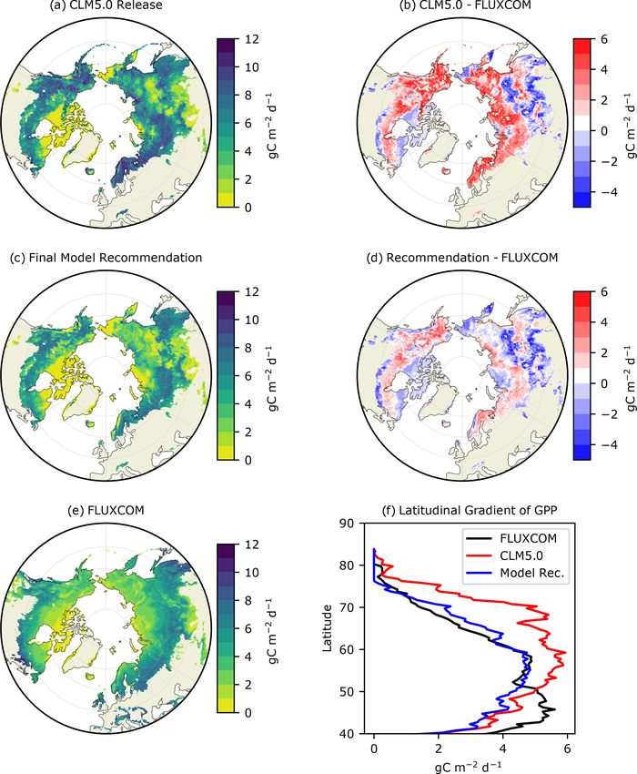
Figure 3. The annual cycle of GPP for CLM5.0 release with intermediate model development steps compared to FLUXCOM for (a) aggre-
gated gridded CLM5.0 output, (b) NET, (c) NDT, (d) BDT, (e) shrubs, and (f) grasses. “Phenology” incorporates changes to onset and offset.
“Param. Scaling” adds our scaling of Jmax and Vcmax by daylight and the Leuning parameterization. “Carbon allocation” adds changes
to the root-to-leaf and stem-to-leaf parameters. The final model recommendation (“Model Rec.”) incorporates the bug fix (Sect. S3 in the
Supplement) and spring initialization of Jmax and Vcmax .
Leuning (2002) as used in CLM4.5, we find that GPP is de- and BDT), approaching FLUXCOM values (Fig. 3). The rest
creased for all PFTs, especially in spring when the photosyn- of our changes to the model involve schemes in LUNA that
thesis ramp-up had been artificially high. Our updated model we believe are initialized incorrectly for the ABZ, but also
improves phenology of NETs due to more realistic scaling of the rest of the world. These recommended model updates in-
Jmax and Vcmax (Fig. 3b, the light blue “Temp Scaling” sim- clude initializing the winter default values of Jmax and Vcmax
ulation and Fig. S12 in the Supplement). The GPP of grasses using the mean value for a given grid cell during the previous
is also decreased (Fig. S13 in the Supplement), but shrubs growing season (Eqs. 4 and 5 and Fig. S4 in the Supplement)
are still biased high. and a model error related to the calculation of 10 d leaf tem-
After decreasing productivity of all PFTs (Fig. 3, com- perature (Sect. S3 in the Supplement).
pare the red “CLM5.0 Release” with the blue “Param. Scal-
ing”), tundra shrub and grass productivity in CLM5.0 re- 3.3 Improved carbon fluxes in the model
tains a substantial high GPP bias (Fig. 3e and f), while the recommendation
deciduous tree PFTs have a low GPP bias (Fig. 3c and d),
which may be related to non-optimized ABZ carbon allo- Based on our changes to phenology, photosynthesis, and car-
cation parameters. Allowing for a dynamic stem-to-leaf al- bon allocation schemes, we recommend the following mech-
location improves both the timing and magnitude of pho- anistically based changes to CLM5.0 for a considerably im-
tosynthesis (Fig. S9 in the Supplement). Additionally, we proved representation of CO2 fluxes in the ABZ:
make PFT-specific alterations to root-to-leaf ratios based on
our findings from Sect. 2.4. As a result, GPP is lowered in
grasses and shrubs and increased for deciduous trees (NDT 1. GPP onset is based on soil temperature, air temperature,
and snow cover.
Geosci. Model Dev., 14, 3361–3382, 2021 https://doi.org/10.5194/gmd-14-3361-2021L. Birch et al.: CLM5.0 biases in the ABZ 3371
2. GPP offset is based on a latitudinal photoperiod gradient
such that the high Arctic begins senescence earlier.
3. Jmax is scaled by maximum day length instead of a con-
stant 12 h.
4. Jmax and Vcmax are scaled by temperature response
functions parameterized by Leuning (2002).
5. Jmax and Vcmax have initial values in spring that are
based on the LUNA predictions from the previous grow-
ing season, allowing the values to vary across PFTs,
time, and space.
6. The stem-to-leaf carbon allocation ratio for trees and
shrubs is allowed to be dynamic throughout the season.
7. Observationally based root-to-leaf carbon allocation ra-
tios are used. For deciduous tree PFTs, the root-to-leaf
ratio is decreased, while the ratio for shrubs and grasses
is increased.
We first validate that our modifications to CLM5.0 offer
improvements to simulations of CO2 fluxes when looking
at specific flux towers (Fig. 4). For instance, productivity is
increased for BDTs at CA-OAS, which is further validated
at CA-GRO. The dead zone at CA-QC2 is now highly pro-
ductive and much closer to observed carbon fluxes in terms
of seasonality and magnitude. The new cold deciduous on-
set scheme causes this improvement, as the previous grow-
ing degree-day scheme in CLM5.0 prevented photosynthesis Figure 4. Comparison of GPP at flux tower sites to the CLM5.0
from ever starting. Photosynthesis in NDTs is increased due release and the results of our model development. We performed
model development at CA-QC2 (mixed forest site in Quebec), CA-
to our model development, but as shown in both gridded out-
OAS (Aspen forest in Saskatchewan), US-EML (Eight Mile Lake
put and RU-SKP, the NDT photosynthesis needs to increase tundra location), and RU-SKP (Yakutsk Spasskaya Larch Forest).
further. The phenology and magnitude of NET is much im- We did additional comparisons with FI-SOD (Sodankylä, Finland),
proved at validation sites. However, as is expected (Schaefer RU-TKS (Tiksi grasslands), CA-SF1 (Saskatchewan boreal forest),
et al., 2012), not all of the flux tower sites have CO2 fluxes RU-COK (Chokurdakh Tundra shrubs), RU-SAM (Samoylov grass-
that are reproduced within the range of observational uncer- lands), and CA-GRO (Groundhog River Boreal Forest).
tainty (Figs. 4c and S11 in the Supplement). For example,
although GPP at US-EML is reduced due to our model de-
velopment, it is still biased high. However, the grasses and shrubs, and grasses. In contrast, our model development suc-
shrubs at other validation sites are much improved compared cessfully delays the onset of productivity in NETs, due to a
to flux measurements, like the grasses and shrubs at RU- combination of daylight scaling and the temperature scaling
SAM, RU-TKS, and US-ATQ. from Leuning (2002). As for the magnitude of photosynthe-
We next compare our model improvements in a gridded sis, we find that NET photosynthesis is reduced across the
simulation against CO2 fluxes from FLUXCOM (Fig. 2a). ABZ, while the deciduous boreal tree PFTs experience an
The high productivity bias at high latitudes is substantially increase in productivity (Fig. S10 in the Supplement).
reduced due to our model development by decreasing the Although GPP is our main focus of development due to
productivity of ABZ shrubs and grasses. Our model rec- the number of productivity biases, we find improvements in
ommendation for CLM5.0 produces a latitudinal gradient other component CO2 fluxes. Changes in TER generally fol-
(Fig. 1f) in productivity, with the tundra no longer being as low those of GPP, and our modifications substantially reduce
productive as the boreal forest (Fig. 3). The timing of pho- the high summer respiration bias in CLM5.0 (Fig. 2), which
tosynthesis is also improved as dormancy is reached by Oc- is mostly due to the reduction of GPP and TER in grasses
tober in most PFTs, instead of November (Figs. 1 and 3). and shrubs at high latitudes (Fig. S6 in the Supplement). The
In examining the PFT-specific output (Fig. 3), we confirm an respiration of deciduous tree PFTs did not change substan-
earlier beginning to spring photosynthesis in deciduous trees, tially, but TER decreases in NETs due to the decrease in
https://doi.org/10.5194/gmd-14-3361-2021 Geosci. Model Dev., 14, 3361–3382, 20213372 L. Birch et al.: CLM5.0 biases in the ABZ
GPP. Due to the improvements in GPP onset and offset, the 4 Discussion
model no longer simulates large net CO2 emissions in spring
(Fig. S7 in the Supplement), which better matches observa- Through mechanistic model development, we have reduced
tions of NEE. In many PFTs the respiration and thus NEE the biases in carbon cycling in CLM5.0 for the Arctic–boreal
in fall are high in the gridded output. Although this does not PFTs. Many of our recommendations in Sect. 2.4 affect sev-
match FLUXCOM, it is consistent with recent measurements eral of the biases noted in Sect. 3.1, indicative of the many in-
of high fall respiration in the ABZ (Commane et al., 2017; terconnected schemes in CLM5.0. Ultimately, we believe our
Natali et al., 2019). The net balance of carbon fluxes does modifications to be reasonable, observationally based, and a
not change substantially due to our model development. We step towards a more accurate simulation of carbon cycling in
find that the carbon sink in ABZ CLM5.0 decreases by about high-latitude terrestrial ecosystems, but we also discuss the
12 %, which is due to a smaller net sink in the summer and limitations of our model development choices and identify
larger carbon release in fall. avenues of research that could continue to improve CLM5.0.
Having more accurate phenology in CLM5.0 is critical for
3.4 Validation with ILAMB understanding the recent and future changes in biogeochem-
istry in the ABZ, as global change drivers during the shoul-
Comparing output from CLM5.0 and our model recommen- der seasons may be drivers of carbon cycle changes. Decid-
dation to observational data provided by the ILAMB frame- uous trees have protective mechanisms to avoid the onset
work confirms broad improvements in model fidelity (Fig. 5). of growth when there is a strong probability of cold snaps
This includes the CO2 fluxes we focus development on, as (McMillan et al., 2008), and our new thresholds are key en-
well as surface fluxes (sensible heat, latent heat, albedo). IL- vironmental conditions designed to mimic the end-of-winter
AMB confirms that the high GPP bias and late phenology signals. The use of threshold values in onset schemes is a
biases are reduced. LAI, in particular, has been improved well established phenology method (Jolly et al., 2005; Arora
greatly in the Arctic in regards to both timing and magnitude and Boer, 2005) that is used in other models, like LPJ (Forkel
(Fig. 5). According to the ILAMB score, the implemented et al., 2014) and the Canadian Terrestrial Ecosystem Model.
changes are not detrimental to any other essential land sur- These schemes can be fairly simple or more complicated,
face variables, and in fact improve their simulation accord- much like growing degree-day (GDD) models. We choose
ing to the centralized benchmark scores. Breaking down the to focus on environmental thresholds due to the uniqueness
overall benchmark score, our model recommendation shows of the ABZ environment, which is dominated by freeze–thaw
large improvements in the spatial distribution and interan- dynamics, making a threshold approach effective. We did in-
nual variability scores. The seasonal cycle score of GPP did vestigate other GDD schemes, but we found that many GDD
not improve substantially, which makes sense due to the phe- models perform similarly (Hufkens et al., 2018) and in the
nology problems only becoming apparent in the PFT-specific ABZ have a documented late onset (Botta et al., 2000; Fu
output, which is not a standard ILAMB benchmark. The et al., 2014), just like the current scheme in CLM5.0. We
NEE seasonal cycle is substantially improved according to did not identify a scheme well validated in the ABZ, as most
ILAMB, which agrees with our FLUXCOM validation. The observational validation studies are focused on the lower lati-
relative improvements to moisture and heat fluxes are par- tudes, and those studies also identify that gridded phenology
ticularly noteworthy, as these changes can feed back to the products tend to be produced using optical imagery, which
regional climate system. often does not correspond well with CO2 fluxes in shoul-
We are also interested in contributing to the improvement der seasons (Fisher et al., 2007; Parazoo et al., 2018a). Ul-
of the global CLM5.0 simulation. We confirm that a global timately, using another GDD scheme from the known liter-
simulation is possible and reasonable (Fig. 6) with these ad- ature would be trading one extrapolated temperate scheme
ditions to the code base. All but two of our model improve- for another. This threshold approach may have limitations
ments are limited to the ABZ, meaning that we do not ex- for a warming world, which is why an ABZ-focused phenol-
pect significant biases to emerge at lower latitudes due to ogy study, using novel datasets like PhenoCam (Richardson
our model development, and our ILAMB validation con- et al., 2018; Hufkens et al., 2018) has potential to uncover
firms this. The constant LUNA equation is one of the global more complicated vegetation processes and filling in gaps
changes and the other is the change in temperature scaling from satellite-based studies (Fisher et al., 2007).
from Kattge and Knorr (2007) to Leuning (2002). Additional Implementing an offset scheme with a latitudinal gradi-
testing at lower latitudes, which is outside of the scope of ent in CLM5.0 is a first step towards more realistic timing
this study, is necessary to determine the effects on the global of fall senescence in CLM5.0, and additional work is needed
carbon budget. to understand how temperature and other climate drivers im-
pact the timing of dormancy. Studies are divided on the issue
of whether temperature or photoperiod are driving offset in
the ABZ. Field experiments have found photoperiod to be a
likely driver at high latitudes (Eitel et al., 2019), but temper-
Geosci. Model Dev., 14, 3361–3382, 2021 https://doi.org/10.5194/gmd-14-3361-2021You can also read