SCALING AND BALANCING CARBON DIOXIDE FLUXES IN A HETEROGENEOUS TUNDRA ECOSYSTEM OF THE LENA RIVER DELTA - MPG.PURE
←
→
Page content transcription
If your browser does not render page correctly, please read the page content below
Biogeosciences, 16, 2591–2615, 2019
https://doi.org/10.5194/bg-16-2591-2019
© Author(s) 2019. This work is distributed under
the Creative Commons Attribution 4.0 License.

Scaling and balancing carbon dioxide fluxes in a heterogeneous
tundra ecosystem of the Lena River Delta
Norman Rößger1 , Christian Wille2 , David Holl1 , Mathias Göckede3 , and Lars Kutzbach1
1 Institute
         of Soil Science, University of Hamburg, Allende-Platz 2, 20146 Hamburg, Germany
2 German Research Centre for Geosciences, Telegrafenberg, 14473 Potsdam, Germany
3 Max Planck Institute for Biogeochemistry, Hans-Knöll-Straße 10, 07745 Jena, Germany

Correspondence: Norman Rößger (norman.roessger@uni-hamburg.de)

Received: 14 January 2019 – Discussion started: 19 February 2019
Revised: 21 May 2019 – Accepted: 30 May 2019 – Published: 5 July 2019

Abstract. The current assessments of the carbon turnover in        sites, the decomposed fluxes were employed in a vegetation
the Arctic tundra are subject to large uncertainties. This prob-   class area-weighted upscaling that was based on a classified
lem can (inter alia) be ascribed to both the general shortage      high-resolution orthomosaic of the flood plain. In this way,
of flux data from the vast and sparsely inhabited Arctic re-       robust budgets that take the heterogeneous surface character-
gion, as well as the typically high spatiotemporal variabil-       istics into account were estimated. In relation to the average
ity of carbon fluxes in tundra ecosystems. Addressing these        sink strength of various Arctic flux sites, the flood plain con-
challenges, carbon dioxide fluxes on an active flood plain         stitutes a distinctly stronger carbon dioxide sink. Roughly
situated in the Siberian Lena River Delta were studied dur-        42 % of this net uptake, however, was on average offset by
ing two growing seasons with the eddy covariance method.           methane emissions lowering the sink strength for greenhouse
The footprint exhibited a heterogeneous surface, which gen-        gases. With growing concern about rising greenhouse gas
erated mixed flux signals that could be partitioned in such a      emissions in high-latitude regions, providing robust carbon
way that both respiratory loss and photosynthetic gain were        budgets from tundra ecosystems is critical in view of accel-
obtained for each of two vegetation classes. This downscal-        erating permafrost thaw, which can impact the global climate
ing of the observed fluxes revealed a differing seasonality in     for centuries.
the net uptake of bushes ( − 0.89 µmol m−2 s−1 ) and sedges
(−0.38 µmol mm−2 s−1 ) in 2014. That discrepancy, which
was concealed in the net signal, resulted from a compara-          1   Introduction
tively warm spring in conjunction with an early snowmelt
and a varying canopy structure. Thus, the representativeness       Permafrost underlies between 12.8 % and 17.8 % of the land
of footprints may adversely be affected in response to pro-        area in the Northern Hemisphere (Zhang et al., 2000). Large
longed unusual weather conditions. In 2015, when air tem-          parts of this area coincide with the Arctic tundra, which is
peratures on average corresponded to climatological means,         situated north of the boreal treeline and covers roughly 8 %
both vegetation-class-specific flux rates were of similar mag-     of the global land surface (McGuire et al., 2012). As a con-
nitude (−0.69 µmol m−2 s−1 ). A comprehensive set of mea-          sequence of the long-term carbon sink function, the underly-
sures (e.g. phenocam) corroborated the reliability of the par-     ing permafrost forms a carbon stock of global relevance: ap-
titioned fluxes and hence confirmed the utility of flux de-        proximately 1300 Gt of soil organic carbon are stored in the
composition for enhanced flux data analysis. This scrutiny         circumpolar permafrost region (Hugelius et al., 2014). How-
encompassed insights into both the phenological dynamic of         ever, large fractions of this carbon pool may be remobilised
individual vegetation classes and their respective functional      in response to a warming climate, making the tundra a key
flux to flux driver relationships with the aid of ecophysiolog-    ecosystem for climate change (Schuur et al., 2008).
ically interpretable parameters. For comparison with other

Published by Copernicus Publications on behalf of the European Geosciences Union.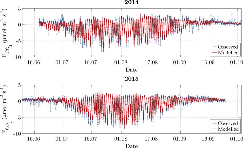
2592                  N. Rößger et al.: Scaling and balancing carbon dioxide fluxes in a heterogeneous tundra ecosystem

   The Arctic north of 60◦ N latitude has warmed at a rate         mate change. Such assessments are based on biome-level
of 1.36 ◦ C per century since 1875, i.e. roughly twice as fast     monitoring of the global warming-induced impacts on Arc-
as the global average (Masson-Delmotte et al., 2013). And          tic vegetation such as growing season prolongation as well
this rapid warming trend is projected to continue (Collins et      as expansion of plant’s growing range and size, e.g. the en-
al., 2013). Due to ambiguous model results and their large         hanced growth of shrubs and their northward migration into
confidence intervals, it currently remains unclear whether         typical graminoid tundra ecosystems (Jia et al., 2009; Sweet
the permafrost areas maintain their sink function or con-          et al., 2015). On the other side, microscale observations
vert into a carbon source in the future (Heimann and Re-           are crucial in order to reflect the individual biogeochemi-
ichstein, 2008; Schuur et al., 2015). These uncertainties do       cal dynamics in the mosaic of vegetation patches. The direct
not only arise from the limited knowledge of the physical          appraisal of the vegetation’s responses to global warming
thawing rates, the fraction of released carbon after thawing       through field surveys on the plant community level involves
and the timescales of release but also from the general short-     aspects such as enhanced primary productivity, deeper root-
age of flux data in Arctic ecosystems (Ciais et al., 2013).        ing depths, as well as augmented ground shading and snow
The scarce data availability particularly applies to the exten-    accumulation trough taller growth forms (Myers-Smith et al.,
sive Siberian tundra, which covers around 3 million km2 , i.e.     2011; Sitch et al., 2007).
more than half of northern high-latitude tundra ecosystems            Chamber measurements operate on the microscale (10−2 –
(Chapin et al., 2005; Sachs et al., 2010). The low density of      102 m2 ) and form the common approach to differentiate the
flux observation sites is due to both harsh environmental con-     carbon dioxide exchange of multiple microforms (i.e. indi-
ditions as well as challenging logistics in these remote and       vidual land cover components such as bare soil, water bod-
sparsely inhabited areas that are often without line power.        ies, vascular plants, etc.) with the atmosphere (McGuire et
Consequently, current estimates of the tundra’s sink strength      al., 2012). Despite their widespread application, however,
for carbon dioxide are associated with large uncertainties:        chamber measurements are associated with several draw-
−103 ± 193 Tg C yr−1 (McGuire et al., 2012). The same is-          backs such as (i) a disturbance of the studied system due to
sue applies to estimates that indicate a shift to a source for     collar insertion, (ii) a subjectivity in the selection of cham-
carbon dioxide: 462 ± 378 Tg C yr−1 (Belshe et al., 2013).         ber locations, which is particularly momentous, if an upscal-
The refinement of these macroscale estimates and the reduc-        ing of fluxes is intended, (iii) a lacking acquisition of a pro-
tion of their uncertainties can be achieved via providing both     nounced temporal flux variability on account of a usual con-
more flux budgets (in particular from the Siberian tundra)         finement to discrete sampling, (iv) a limited spatial repre-
and more reliable information on the variation in habitats         sentativeness due to both the small sampled size and only a
(e.g. bogs, fens,) plus their associated surface heterogeneities   few replicate sites as a result of a high labour intensity, and
(e.g. tussocks, hummocks).                                         (v) a decoupling of the sampled surface from the atmosphere
   Tundra ecosystems are frequently characterised by a pro-        that causes a modification of the environmental conditions in
nounced vegetation patchiness with sharply defined bound-          the headspace (Fox et al., 2008; Kade et al., 2012; Kutzbach
aries between different vegetation classes (Shaver et al.,         et al., 2007a; Livingston et al., 2006; Riederer et al., 2014;
2007). Besides vegetation, surface classifications can also        Sachs et al., 2008; Wagner and Reicosky, 1992).
be based on differences in soil moisture, snow cover, per-            Alternatively, the non-intrusive as well as directly and con-
mafrost features or combinations of them (Fox et al., 2008;        tinuously measuring eddy covariance technique circumvents
Virkkala et al., 2018). The consequently high spatial vari-        most of these downsides. This method, however, operates on
ability in carbon fluxes complicates the estimation of robust      the mesoscale (104 –106 m2 ) and yields turbulent fluxes that
carbon budgets that are accurate and precise. The omission         integrate across multiple microforms (Aubinet et al., 2012).
of accounting for the spatial distribution of different sur-       The size and location of the sampled surface constantly shifts
face types is likely to lead to incorrect budgets (Oechel et       according to wind direction, wind speed, atmospheric stabil-
al., 1998). Therefore, an improved understanding of the ef-        ity, crosswind velocity and surface roughness (Detto et al.,
fects of surface heterogeneity on these budgets, e.g. through      2006). In the presence of a heterogeneous landscape (i.e. an
a better characterisation of both spatial flux variability as      irregular pattern of individual land cover components), the
well as associated key factors such as vegetation composi-         temporal variability in the observed fluxes is not only a result
tion and structure, is necessary (Kade et al., 2012; Kwon          of the varying uptake/release rates of the individual micro-
et al., 2006). For quantifying vegetation properties, NDVI         forms but also an outcome of the varying fractions of micro-
(normalised difference vegetation index), LAI (leaf area in-       forms in the sampled area. In addition, the footprint budgets
dex) and foliar nitrogen content have been found suitable          may lack representativeness since the fractional composition
(Marushchak et al., 2013; Shaver et al., 2013). All of these       of microforms within the footprint is likely to deviate from
predictors can be estimated by remote sensing, thereby ne-         the microform distribution in the area of interest. In such
glecting the patchy nature of tundra ecosystems, but also of-      an environment, budgets strongly depend on tower location,
fering the potential for macroscale modelling of both carbon       sensor height and wind field conditions, and are thus likely
dioxide budgets plus their prospective alterations through cli-    to exhibit a sensor location bias (Schmid and Lloyd, 1999).

Biogeosciences, 16, 2591–2615, 2019                                                     www.biogeosciences.net/16/2591/2019/
N. Rößger et al.: Scaling and balancing carbon dioxide fluxes in a heterogeneous tundra ecosystem                                2593

Moreover, heterogeneous flux signals also complicate the             tumn). More importantly, the surface of the flood plain ex-
determination of model parameters, e.g. the light response           hibits, in opposition to the river terrace, a distinct heterogene-
curve of a specific vegetation type, if the microforms in the        ity on the mesoscale.
footprint exhibit strongly deviating characteristics (Lasslop           The central delta region is situated in a continental Arc-
et al., 2010). Despite these challenges in signal interpreta-        tic climate, which is characterised by very low tempera-
tion, a heterogeneous surface also provides the opportunity to       tures and a low annual precipitation. In the distant town
both conduct a concurrent sampling of multiple microforms            of Tiksi, located around 120 km southeast of Samoylov Is-
and study their respective carbon dioxide fluxes utilising only      land, a mean annual air temperature of −12.8 ◦ C was mea-
one eddy covariance instrumentation (Forbrich et al., 2011;          sured during 1936–2016 and a mean annual precipitation of
Morin et al., 2017). Exploiting this potentially valuable in-        329 mm was gauged during 1956–2016 (AARI, 2017). Addi-
formation source requires the partitioning of the integrated         tional information on this study site can be found in Rößger
flux into its microform-specific fluxes. Such a successful flux      et al. (2019a).
decomposition routine benefits from the advantages of eddy
covariance measurements on the mesoscale whilst resolving            2.2   Experimental setup and data recording
the pronounced variability on the microscale. These decom-
posed fluxes in turn enable, in conjunction with a precise de-       An eddy covariance system was installed in the southern
termination of the microforms’ spatial coverages in the area         part of the flood plain, and the measurements covered two
of interest, the estimation of robust carbon dioxide budgets         periods: 18 June to 2 October 2014 (107 d) and 9 June to
for a heterogeneous surface.                                         24 September 2015 (108 d).
   Addressing the problems of balancing carbon fluxes in a               The flux tower was equipped with a sonic anemometer
Siberian tundra ecosystem with both a heterogeneous surface          (CSAT3, Campbell Scientific, UK) and a gas analyser for
and an unknown greenhouse gas sink/source strength, the ob-          water vapour and carbon dioxide (LI-7500A, LI-COR Bio-
jectives of this study are as follows: (i) elucidating the hetero-   sciences, USA). Both instruments were mounted at a height
geneity of the landscape with geospatial data, (ii) analysing        of 2.83 m and sampled with a frequency of 20 Hz. In addi-
the spatiotemporal variability of carbon dioxide fluxes with         tion, another eddy covariance system with the same instru-
the eddy covariance technique, (iii) explaining this variabil-       mentation has already been deployed at a central position on
ity with a model-based approach, (iv) estimating robust car-         the adjacent river terrace (Holl et al., 2019).
bon dioxide budgets that account for the heterogeneity of the            Supplementary measurements on the flood plain involved
area, and (v) combining these budgets with previously esti-          gathering data of both air temperature (HMP45, Camp-
mated methane budgets in order to determine the sink/source          bell Scientific, UK) and photosynthetic photon flux density
strength for greenhouse gases.                                       (SKP215, Skye Instruments, UK). These environmental vari-
                                                                     ables were recorded on a logger (CR1000, Campbell Scien-
                                                                     tific, UK) in quarter-hourly intervals. Furthermore, a time-
2     Material and methodology                                       lapse camera (TLC200, Brinno, Taiwan) was mounted on the
                                                                     flux tower, pointing northeast, for monitoring the phenology
2.1    Site description                                              during spring 2014 with the same interval of a quarter of an
                                                                     hour.
The Lena River Delta, one of the largest deltas in the world, is         An acquisition of data on the footprint’s surface struc-
located within the zone of continuous permafrost in northern         ture was intended by employing ground-based LAI mea-
Siberia (Fig. 1). One of its numerous islands is Samoylov Is-        surements, as this quantity is widely applied for characteris-
land (72◦ 220 N, 126◦ 280 E), which covers an area of 4.8 km2        ing plant canopies. However, on account of the low height
and features two geomorphological units: the Late Holocene           of lichens, mosses and sedges, the measurements with an
river terrace in the eastern part and the active flood plain         upwards-pointing sensor (LAI-2200C, LI-COR Biosciences,
in the western part. The carbon dioxide exchange on the              USA) yielded poor quality results. Therefore, the measure-
river terrace, which is characterised by ice-wedge polyg-            ments were terminated after a few test surveys.
onal tundra with sedges and mosses, has been repeatedly
studied (Eckhardt et al., 2019; Kutzbach et al., 2007b; Run-         2.3   Flux processing
kle et al., 2013). In contrast to the river terrace, the flood
plain has to date received scarce attention in terms of green-       The flux computation was carried out with the software Ed-
house gas fluxes, although active flood plain levels represent       dyPro version 6.0.0 (LI-COR Biosciences, 2016) for 30 min
roughly 40 % of the soil-covered area of the Lena River Delta        flux intervals and followed the standard procedure. Detailed
(Zubrzycki et al., 2013). Aside from the period of the annual        information on the executed (i) raw data processing (spike
spring flood, whose associated inundation is very variable in        removal, coordinate rotation, block averaging, time lag com-
magnitude and duration, the flood plain on Samoylov Island           pensation), the implemented (ii) flux correction scheme
stretches over an area between 1 km2 (spring) and 2 km2 (au-         (density correction, spectral correction in low- and high-

www.biogeosciences.net/16/2591/2019/                                                         Biogeosciences, 16, 2591–2615, 2019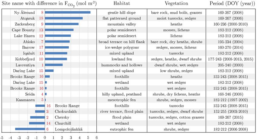
2594                    N. Rößger et al.: Scaling and balancing carbon dioxide fluxes in a heterogeneous tundra ecosystem

Figure 1. Location of the Lena River Delta in northern Siberia indicated by the square. The dots point out sites that were utilised for the pan-
Arctic comparison of carbon dioxide budgets (Table 3). The classification of the Arctic zones was based on vegetation occurrence (modified
from AMAP, 1998). Accordingly, the treeline delimits the (terrestrial) Arctic; i.e. it corresponds with the boundary between sub-Arctic and
low Arctic.

frequency ranges, flux error estimation), and the conducted               2.4    Surface structure
(iii) quality assessment routine (stationarity test, integral tur-
bulence characteristics test, skewness and kurtosis examina-
tion, energy flux quality verification, signal strength control,          For studying the impact of the heterogeneous surface on the
percentile removal) is provided in Rößger et al. (2019a).                 flux variability, the entire flood plain was mapped in August
   For the footprint modelling, an analytical model for non-              2014 by employing helicopter-based visible aerial imagery.
neutral stratification was employed (Kormann and Meixner,                 The resulting geo-referenced orthomosaic exhibited a reso-
2001). This model is based on a stationary gradient diffu-                lution of 8.5 cm and hence provided very detailed spatial in-
sion formulation with height-independent crosswind disper-                formation, which was sufficient to resolve the pronounced
sion (Leclerc and Foken, 2014). When applying the solution                heterogeneity of the surface. Based on maximum likelihood
of the resulting two-dimensional advection–diffusion equa-                classification tools, the vegetation was classified employing a
tion for solving the power law profiles of both eddy diffusiv-            supervised classification routine on the orthomosaic (Fig. 2).
ity and mean wind velocity, it yielded a source weight func-              In this process, four different land cover classes were utilised,
tion for each flux interval.                                              two of which represent the vegetation.
                                                                             Vegetation class 1 (“shrubs”) refers to sites, which were
                                                                          densely vegetated by large dwarf shrubs of the willow fam-
                                                                          ily such as Salix pulchra, Salix lanata, Salix hastata, Salix
                                                                          glauca, growing to a maximum height of around 1 m. This
                                                                          shrubby vegetation was located on a sandy ridge aligned

Biogeosciences, 16, 2591–2615, 2019                                                              www.biogeosciences.net/16/2591/2019/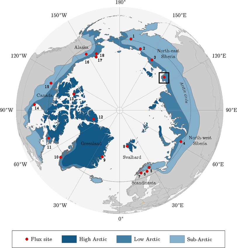
N. Rößger et al.: Scaling and balancing carbon dioxide fluxes in a heterogeneous tundra ecosystem                                                  2595

                                                                        ter levels up to 40 cm. The ample moisture attracted many
                                                                        mosses forming a dense cover of thick moss.
                                                                           The two other classes, which do not occur in the 90 %
                                                                        contribution footprint around the flux tower, denote a large
                                                                        area of bare sand along the waterfront and some small wa-
                                                                        ter bodies mainly situated in the northern part of the flood
                                                                        plain (Fig. 2). The former class was not considered in the
                                                                        budget estimation since its carbon dioxide flux rates were (in
                                                                        comparison to the two vegetation classes) assumed negligi-
                                                                        ble. The latter class was appended to vegetation class 2 as
                                                                        the few small water bodies surrounded by sedges were pre-
                                                                        sumed to have similar flux rates. Further information on the
                                                                        classification routine is given in Rößger et al. (2019a).

                                                                        2.5   Flux modelling

                                                                        The model structure was based on the computation of the two
                                                                        components of the carbon dioxide flux.
                                                                        FCO2 = NEE = TER − GPP                                                      (1)
                                                                        FCO2 is the net carbon dioxide flux observed at the flux tower
                                                                        and is equal to the net ecosystem exchange (NEE). Its two
                                                                        components describe, respectively, the total ecosystem res-
                                                                        piration (TER) and the gross primary productivity (GPP),
                                                                        both of which can be modelled simultaneously (Runkle et
                                                                        al., 2013).

                                                                                               Tair −Tref
                                                                                                    γ               Pmax · α · PPFD
                                                                        NEE = Rbase · Q10                       −                                   (2)
                                                                                                                    Pmax + α · PPFD
                                                                        Rbase denotes the basal respiration at the reference tempera-
Figure 2. Vegetation map of the flood plain on Samoylov Island          ture (Tref ), which was set to 15 ◦ C, and a scaling factor (γ )
obtained through supervised classification of a high-resolution or-     was held constant at 10 ◦ C (Mahecha et al., 2010). Q10 indi-
thomosaic. The flux tower was situated in the centre of the footprint   cates the temperature sensitivity; i.e. this parameter is a value
isolines, which indicate the averaged area from which 10 %–90 %         by which respiration multiplies/divides, when the tempera-
(increments of 10 %) of the flux originated during the measurement      ture rises/drops by 10 ◦ C. Pmax refers to the maximum pho-
periods of 2014 and 2015 (footprint climatology). The small inset
                                                                        tosynthetic potential and quantifies the theoretical maximum
illustrates Samoylov Island being composed of flood plain (grey)
                                                                        of photosynthesis at infinite irradiance. α represents the light
and river terrace (white) plus the location of their respective flux
towers.                                                                 sensitivity and states, as the initial quantum efficiency, the
                                                                        slope of the light response curve at irradiance of zero. All of
                                                                        the four (physiologically interpretable) parameters are best-
in the north–south axis. The elevated area enabled, in con-             fit parameters, which were estimated via non-linear ordinary
junction with a spatially averaged maximum thaw depth of                least-squares regression utilising both air temperature (Tair )
0.93 m, a good drainage. Since the groundwater table re-                and photosynthetic photon flux density (PPFD) as explana-
mained at depths around 50 cm, the surface was mostly dry,              tory variables. In order to take the heterogeneous surface
forming favourable growing conditions for willow shrubs                 structure into account, footprint information was included,
and a sparse cover of thin moss.                                        forming the final model employed for carbon dioxide flux
   Vegetation class 2 (“sedges”) represents areas, which were           modelling.
dominated by sedges including Carex aquatilis, Carex chor-                      i=2
                                                                                X
dorrhiza, Carex concolor, as well as species of Eriopho-                NEE =         i
rum and Equisetum. Also, small willow shrubs growing to                         i=1

                                                                                                       Tair −Tref
                                                                                                                                              !
a height of about 0.3 m were occasionally to be found. This                                                 γ             Pmax,i · αi · PPFD
predominantly graminoid vegetation was located in depres-                       · Rbase,i · Q10,i                       −                           (3)
                                                                                                                          Pmax,i + αi · PPFD
sions around the dry ridge and exhibited a mean active layer
depth of 0.69 m. Accordingly, the soil moisture conditions              Another explanatory variable is the relative contribution of
alternated between moist surfaces and wet patches with wa-              each vegetation class to the flux () that weights the two

www.biogeosciences.net/16/2591/2019/                                                                   Biogeosciences, 16, 2591–2615, 2019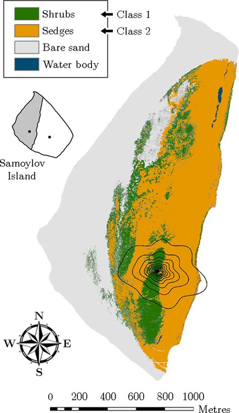
2596                   N. Rößger et al.: Scaling and balancing carbon dioxide fluxes in a heterogeneous tundra ecosystem

computed vegetation-specific fluxes. This variable was ob-           plausible best-fit parameters were in. The output was tested
tained through (i) computing the source weight function for          again, and in case of significant best-fit parameters, the mod-
a flux interval, (ii) spatially discretising this continuous func-   elled NEE was accepted, and the fitting procedure continued
tion with a resolution of 1 m, (iii) adjusting the vegetation        with the next day. Lastly, a replacement function for Pmax
map to a resolution of 1 m, (iv) assigning each value of the         was created by fitting a Gaussian bell curve to the time series
source weight function to its spatially corresponding vege-          of significant best-fit Pmax values in both vegetation classes.
tation class, and (v) summing the values in each vegetation          In the final step (step 4), two greatly simplified models (2-
class.                                                               1-p/1-2-p) were run with only three fitting parameters to be
    The fitting procedure, in which only half-hourly quality-        estimated, as well as a Pmax value from the replacement func-
controlled flux data were employed, required the estimation          tion. Here, if not before, all fitting parameters have taken on
of a large number of fitting parameters: Rbase , Q10 , Pmax , α      meaningful and significant values, which ensured the com-
for each vegetation class (Fig. 3). In order to avoid overpa-        putation of reliable NEE values. In addition to this brief ex-
rameterisation and equifinality problems, the model structure        planation, a detailed description of the entire fitting process
was gradually simplified along four different steps. These al-       is attached in the Appendix.
terations in the parameterisation enabled the desired estima-           Since the model was designed to simultaneously compute
tion of (i) reasonable seasonal courses of the fitting parame-       the component fluxes in both vegetation classes, it provided
ters, i.e. courses that displayed a predominantly smooth evo-        the capability for the decomposition of the observed fluxes
lution with elevated values during the growing season and            into their separate flux contributions by the two vegetation
low values in the shoulder seasons, and (ii) meaningful and          classes. The reliability of this downscaling, however, was de-
significant values for the fitting parameters, i.e. values that      pendent on the restrictive acceptance of meaningful and sig-
were within an acceptable range and their 95 % confidence            nificant values for the fitting parameters. The temporal inte-
interval did not overlap zero. Achieving both objectives pro-        gration of these partitioned fluxes and the subsequent projec-
vided the possibility to interpret the fitting parameters eco-       tion of the resulting budgets on their corresponding areas on
physiologically.                                                     the flood plain formed the upscaling. The summation of both
    In each of the four parameterisation steps, the respectively     vegetation class budgets finally yielded a robust budget of the
parameterised model was recalibrated for every day, applying         entire flood plain, which was designated as the area of inter-
a moving window with fixed/flexible window sizes and a step          est. This budget, as opposed to the directly estimated foot-
size of 1 d. In the initial step (step 1), which served the com-     print budget, did not exhibit a sensor location bias and hence
putation of representative Q10 values, all of the eight fitting      allowed an unbiased appraisal of both the interannual vari-
parameters were estimated in the model (4-4-p). Through its          ability and the sink/source strength. For the sake of compa-
output, which encompassed eight best-fit time series, a repre-       rability of the budgets between the years, the carbon dioxide
sentative Q10 value was obtained for each vegetation class by        budgets were calculated for the comparison period of 18 June
determining the median out of the best-fit Q10 values that ful-      to 24 September, where data were available in both years.
filled two requirements: statistical significance and an asso-       The utilised methane budgets, being necessary for estimating
ciated coefficient of determination (between observed NEE            greenhouse gas sink/source strengths, have been obtained for
and modelled NEE) of 0.75 or greater. These two Q10 val-             the same period and in a similar fashion to the carbon dioxide
ues were held constant in the further fitting procedure. In the      fluxes, i.e. an initial downscaling of the observed net fluxes
subsequent step (step 2), the simplified model (3-3-p) was           and a subsequent upscaling of the decomposed fluxes on the
run with six fitting parameters to be estimated, and a Gaus-         flood plain (Rößger et al., 2019a).
sian bell curve was fitted to the time series of significant best-
fit α values for each vegetation class. By adding/subtracting
30 % of the function values to/from these two replacement            3     Results
functions, a pair of encompassing threshold functions was
respectively appended. These intervals around the replace-           3.1    Meteorological conditions
ment functions formed a range inside which best-fit α val-
ues were accepted. In the following step (step 3), the model         The mean air temperatures during the measurement periods
(3-3-p) was run with the same parameterisation of the pre-           in 2014 and 2015 amounted to 7.7 and 7.1 ◦ C, respectively.
vious step. The model output was checked for α values in-            Furthermore, the respective precipitation sums totalled 92.3
side the acceptable interval as well as significant values for       and 130.4 mm. The assessment of these values was based
Rbase , Pmax and α. If these criteria were satisfied, the accord-    on their comparison with long-term averages that were ob-
ingly modelled NEE was approved, and the fitting procedure           tained for Samoylov Island between 1998 and 2018 (Fig. 4).
proceeded to the next day. Alternatively, several models (3-         The measurement period in 2014 was on average distinc-
2-p/2-3-p/2-2-p) were run employing α value(s) from the re-          tively warmer and slightly drier, while the measurement pe-
placement function(s) for one or both vegetation classes, de-        riod in 2015 featured the same mean temperature as the base-
pending on which vegetation class insignificant and/or im-           line but considerably more rain. The largest differences in air

Biogeosciences, 16, 2591–2615, 2019                                                      www.biogeosciences.net/16/2591/2019/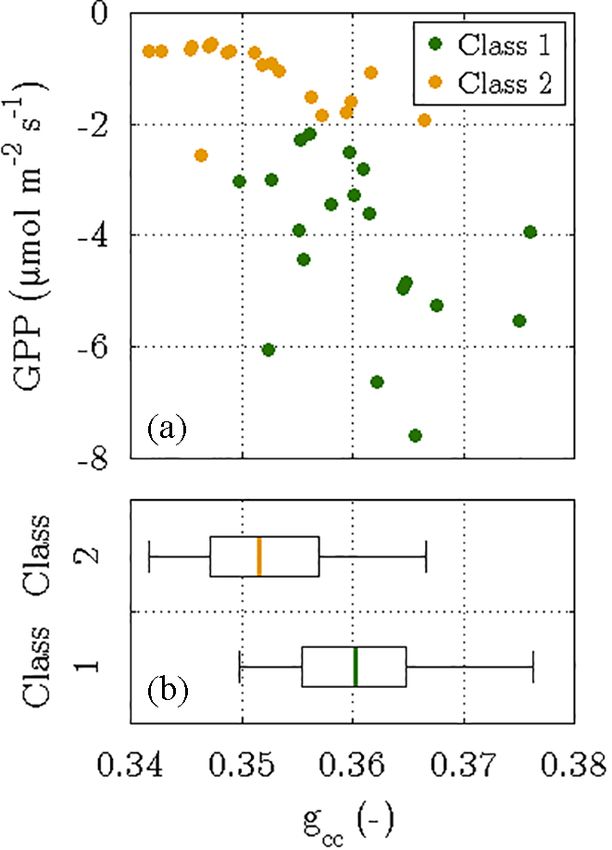
N. Rößger et al.: Scaling and balancing carbon dioxide fluxes in a heterogeneous tundra ecosystem                                         2597

Figure 3. Schematic overview of the model calibration along four steps, in which different parameterisations were applied to obtain mean-
ingful estimates for the eight fitting parameters (Rbase , Q10 , Pmax , α for each vegetation class). The values in the boxes (e.g. 3-2-p model)
denote the number of parameters to be fitted for each vegetation class.

www.biogeosciences.net/16/2591/2019/                                                                Biogeosciences, 16, 2591–2615, 2019
2598                   N. Rößger et al.: Scaling and balancing carbon dioxide fluxes in a heterogeneous tundra ecosystem

Figure 4. Annual course of air temperature on Samoylov Island for the years 2014 and 2015, as well as the recent 20-year baseline (Boike
et al., 2013, 2019). In each box plot, the central mark denotes the monthly median, and the bottom and top edges indicate the 25th and 75th
percentiles, respectively. The whiskers extend to the most extreme data points excluding outliers. During the warm season, when flux data
were available (June to September), 2014 was mostly warmer than 2015.

temperature between both measurement periods occurred in                3.3   Model calibration and performance
spring. Accordingly, the snowmelt in 2014 took place in a
prolonged manner during mid-May already, whereas in 2015,               While the Q10 values were optimised at constant values of
the snowmelt was completed within a couple of days in early             1.42 for vegetation class 1 and 1.48 for vegetation class 2,
June, as usual.                                                         the other fitting parameters (Rbase , Pmax and α) displayed a
                                                                        seasonal course for each vegetation class in 2014 and 2015
3.2    Dynamics of observed fluxes                                      (Figs. 6 and 7). The temporal evolution of α values could be
                                                                        well approximated with replacement functions, whose appli-
The carbon dioxide fluxes exhibited both a diurnal and a                cation reduced the noise not only in the seasonal courses of
seasonal course with the following mean fluxes that were                α but also in the seasonal courses of both Rbase and Pmax . In
obtained by averaging half-hourly flux data for the sub-                contrast to the replacement functions of α, which were cre-
seasons in both 2014 and 2015 (Fig. 5). Between the                     ated for both vegetation classes in both years, a replacement
snowmelt and the vegetative phase, the mean carbon diox-                function for Pmax was created only for vegetation class 1 in
ide fluxes remained slightly positive, indicating a prevalent           2015 and for vegetation class 2 in 2014.
respiration, while the vegetation largely remained dormant                 The slightly simplified 3-3-p model, which was run at the
(0.26 µmol m−2 s−1 ). With the onset of the growing season in           start of step 3, yielded meaningful and significant values for
late June, stalks and foliage began to develop, and the uptake          the fitting parameters in 49 % of the modelled days includ-
of carbon dioxide during daytime outweighed the release                 ing 2014 and 2015 (Fig. 3). In the further course of step 3,
of carbon dioxide during nighttime (−1.06 µmol m−2 s−1 ).               these goals were achieved by the gradually simplified 3-2-
The intensity of this oscillation increased towards the on-             p/2-3-p/2-2-p models in 47 % of the modelled days. During
set of the reproduction phase in mid-July, where flowers                the remaining 4 %, the greatly simplified 2-1-p/1-2-p models
and seeds developed. During this phase, the most nega-                  of step 4 were deployed. While the 3-3-p model was mainly
tive fluxes occurred featuring a relatively constant magni-             employed during the summer season, the 3-2-p/2-3-p/2-2-p
tude (−1.77 µmol m−2 s−1 ). With the onset of the ripening              models were applied throughout the measurement periods
phase in early August, bushes and sedges attained full ma-              with a focus on the shoulder seasons. The 2-1-p/1-2-p models
turity, and the flux amplitude of the diurnal cycle began               were solely deployed during the shoulder seasons and more
to be progressively attenuated (−0.78 µmol m−2 s−1 ). Dur-              often during spring than during autumn. Hence, larger fluxes
ing the nights of this period, the most positive fluxes oc-             during the growing season could be more easily modelled in
curred. Towards late August, the respiration exceeded photo-            comparison to the remaining time, when lower fluxes associ-
synthesis again, indicating the onset of the senescence phase,          ated with a less favourable signal-to-noise ratio prevailed.
which was associated with both leaf colouration and leaf                   Rbase was the fitting parameter that could be estimated
drop (0.39 µmol m−2 s−1 ). After the end of the growing sea-            most confidently, as this parameter accounted for only 19 %
son in early September, when abscission was completed, the              of the insignificant values obtained during the fitting pro-
dominance of respiration continued to grow, leading to more             cedure in 2014 and 2015. While Pmax caused 31 % of the
positive mean carbon dioxide fluxes (0.55 µmol m−2 s−1 ).               insignificance values, α appeared to be the least certain fit-
                                                                        ting parameter representing the remaining 50 %. Further-
                                                                        more, Pmax featured most of the significant differences in
                                                                        best-fit values between both vegetation classes, i.e. the con-

Biogeosciences, 16, 2591–2615, 2019                                                           www.biogeosciences.net/16/2591/2019/
N. Rößger et al.: Scaling and balancing carbon dioxide fluxes in a heterogeneous tundra ecosystem 2599
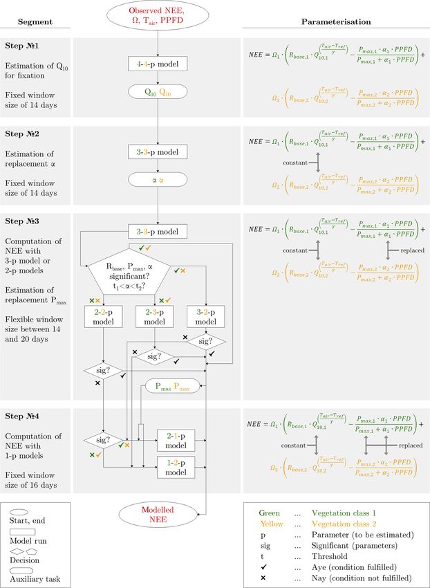
Figure 5. Time series of observed carbon dioxide fluxes (after conducting the quality assessment) and modelled fluxes. During the growing
season, which is indicated by an elevated variability between late June and early September, the daytime uptake directly followed the diurnal
cycle of PPFD, while the nighttime release was dependent on air temperature.
fidence intervals of vegetation classes 1 and 2 rarely over- to early August), when the net uptake of vegetation class 1
lapped, whereas best-fit α values exhibited the fewest signif- was considerably larger relative to vegetation class 2. Dur-
icant differences. ing the second half of the growing season (early August to
On account of both the recalibration for each day as well late September), both net uptakes were rather similar again.
as the coinciding variabilities of explanatory variables and Furthermore, the differences in the net uptakes between both
the explained variable, the model was able to reproduce the years were governed by changes in GPP rather than in TER.
observed fluxes very well (Fig. 5). This performance was ex- In vegetation class 1, NEE in 2014 was only slightly greater
pressed by a coefficient of determination (R 2 ) of 0.88 for in comparison to 2015, which can be attributed to a greater
2014 and 0.95 for 2015. Furthermore, the mean absolute TER and a distinctly greater GPP. And in vegetation class 2,
error (MAE) amounted to 0.49 and 0.35 µmol m−2 s−1 for NEE in 2014 was smaller compared to 2015, which can be
2014 and 2015, respectively, while the root mean square error ascribed to a smaller TER and a clearly smaller GPP.
(RMSE) amounted to 0.75 and 0.52 µmol m−2 s−1 . During The aggregation of the decomposed fluxes over the com-
the summer season, the model performed better in compari- parison period yielded individual budgets, whose multiplica-
son to the shoulder seasons, where autumn in turn displayed tion with the corresponding fractional coverages on the flood
a slightly better performance than spring. plain formed the upscaling (Table 1). The subsequent sum-
mation of both vegetation-class-specific net uptakes returned
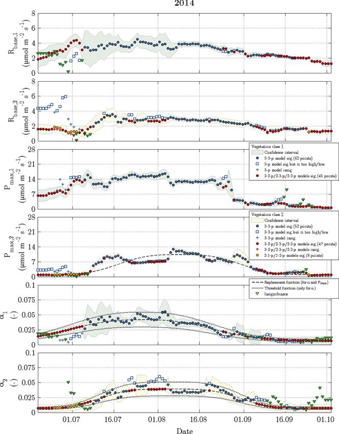
3.4 Downscaling and upscaling of fluxes the net uptake of the entire flood plain for the comparison
period: −4.42 ± 0.49 Mmol in 2014 and −6.17 ± 0.66 Mmol
in 2015. The stated uncertainties were obtained by means of
The estimation of vegetation-class-specific parameter sets
standard error propagation techniques including both cumu-
allowed the decomposition of the observed net fluxes.
lative flux error and classification error, where the former was
This downscaling yielded fluxes of NEE plus their com-
an order of magnitude smaller than the latter. Dividing these
ponent fluxes (TER and GPP) accounting for both vege-
budgets by the total area of the flood plain yielded mean flood
tation classes in both years (Fig. 8). For the comparison
plain budgets of −4.22±0.47 and −5.89±0.63 mol m−2 (Ta-
period in 2014, the mean NEE amounted to −0.89 and
ble 2). These budgets consider the surface heterogeneity; i.e.
−0.38 µmol m−2 s−1 for vegetation class 1 and vegetation
they are corrected for the sensor location bias, plus they con-
class 2, respectively, and for the comparison period in 2015,
tain an areal reference and thus enable an appropriate com-
−0.71 and −0.69 µmol m−2 s−1 (Table 1). In contrast to the
parison with other sites.
similar mean net uptakes in 2015, the mean net uptakes in
2014 distinctly differed from each other. This discrepancy
originated from the first half of the growing season (mid-June
www.biogeosciences.net/16/2591/2019/ Biogeosciences, 16, 2591–2615, 20192600 N. Rößger et al.: Scaling and balancing carbon dioxide fluxes in a heterogeneous tundra ecosystem Figure 6. Time series of fitting parameters in 2014 for vegetation class 1 (index 1 and green confidence intervals) and vegetation class 2 (index 2 and yellow confidence intervals). The circles represent acceptable fits, while the respective reasons for reparameterisation such as insignificant values or values out of valid range are indicated by plus signs and squares. The triangles denote the fitting parameter(s), which caused a refit in the corresponding vegetation class. Biogeosciences, 16, 2591–2615, 2019 www.biogeosciences.net/16/2591/2019/
N. Rößger et al.: Scaling and balancing carbon dioxide fluxes in a heterogeneous tundra ecosystem                               2601

Figure 7. Time series of fitting parameters in 2015 with the same symbols and colours as utilised in the previous figure.

www.biogeosciences.net/16/2591/2019/                                                              Biogeosciences, 16, 2591–2615, 2019
2602                   N. Rößger et al.: Scaling and balancing carbon dioxide fluxes in a heterogeneous tundra ecosystem

Figure 8. Time series of decomposed fluxes with 95 % confidence intervals for both vegetation classes. The width of the confidence intervals
varied depending on both the flux magnitude and the number of fitting parameters in the chosen model. The decomposition revealed a distinct
difference in the net uptake between both vegetation classes during the first half of the growing season in 2014, while the flux dynamics of
both vegetation classes were rather similar during the remaining time and in 2015.

Biogeosciences, 16, 2591–2615, 2019                                                           www.biogeosciences.net/16/2591/2019/
N. Rößger et al.: Scaling and balancing carbon dioxide fluxes in a heterogeneous tundra ecosystem                                                         2603

Table 1. Outcome of downscaling and upscaling carbon dioxide fluxes for the comparison period (18 June to 24 September) in both 2014 and
2015. The mean downscaled fluxes (± standard deviation) refer to the individual fluxes of both vegetation classes (Fig. 8). Their aggregation
yielded cumulative fluxes, whose projection on their corresponding areas on the flood plain in turn returned upscaled fluxes (± combination
of cumulative flux error and classification error). The uncertainty metrics derived from the comparison of the applied vegetation map, which
was obtained through supervised classification of aerial imagery, with another vegetation map that was acquired via ground-based surveys
(Rößger et al., 2019a).

 Vegetation         Fractional    Classification           Downscaled FCO2 (µmol m−2 s−1 )                                Upscaled FCO2 (Mmol)
 class               cover on       uncertainty            2014                       2015                         2014                          2015
              flood plain (m2 )             (%)     NEE      TER    GPP      NEE       TER       GPP      NEE      TER        GPP     NEE        TER      GPP
 1                    251 891              19.1    −0.89    2.62   −3.51    −0.71      1.87     −2.58    −1.89     5.56      −7.45   −1.51    3.96      −5.47
                                                   ±2.86   ±0.84   ±3.32    ±2.51     ±0.99     ±3.11    ±0.36    ±1.06      ±1.42   ±0.29   ±0.75      ±1.04
 2                    795 065              19.5    −0.38    1.81   −2.19    −0.69      2.11     −2.81    −2.53    12.12     −14.65   −4.66   14.11      −18.77
                                                   ±1.81   ±0.71   ±2.21    ±2.32     ±0.68     ±2.62    ±0.33    ±1.55      ±1.87   ±0.59   ±1.81       ±2.41

Table 2. Comparison of the sink/source strengths between flood plain and river terrace for the comparison periods in 2014 and 2015 (Holl
et al., 2019; Rößger et al., 2019a). Accounting for methane’s radiative efficiency as a potent greenhouse gas, the methane budgets were
converted to carbon dioxide equivalents with a factor of 34, which corresponds to methane’s global warming potential based on a time
horizon of 100 years including climate carbon feedbacks (Myhre et al., 2013). The flood plain budgets are given for each vegetation class and
for the total area. These budgets are the result of a scaling procedure, which included fairly large classification errors that caused distinctly
greater uncertainties in comparison to the river terrace budgets, which derived from a representative footprint and hence did not undergo any
scaling processes. In comparison to the flood plain, the polygonal tundra on the river terrace took up less carbon dioxide per square metre,
but also released less methane, resulting in a similar (2014) and weaker (2015) sink strength for greenhouse gases.

  Geomorphological          Vegetation                    FCO2                                     FCH4                            Greenhouse gases
  unit                      class                    (mol CO2 m−2 )                           (mol CH4 m−2 )                      (mol CO2 eq. m−2 )
                                                      2014              2015                   2014               2015               2014                2015
  Flood plain               1                −7.51 ± 1.43      −5.99 ± 1.15         0.004 ± 0.001       0.002 ± 0.001       −7.45 ± 1.43     −5.98 ± 1.15
                            2                −3.18 ± 0.42      −5.86 ± 0.74         0.213 ± 0.042       0.221 ± 0.042       −0.55 ± 0.66     −3.12 ± 0.91
                            Total            −4.22 ± 0.47      −5.89 ± 0.63         0.163 ± 0.032       0.169 ± 0.032       −2.21 ± 0.61     −3.81 ± 0.74
  River terrace             Total            −3.47 ± 0.03      −3.74 ± 0.03         0.096 ± 0.001       0.099 ± 0.001       −2.29 ± 0.03     −2.52 ± 0.03

3.5      Greenhouse gas balances                                                    sink than vegetation class 2 in both years, which is mainly
                                                                                    due to the fact that methane emissions were only present in
The evaluation of the flood plain’s sink/source strength                            vegetation class 2. Since these emissions hardly changed be-
for greenhouse gases required the corresponding methane                             tween the years along with the negligible methane release in
emission budgets and their conversion to carbon dioxide                             vegetation class 1, the interannual variability in the green-
equivalents (Rößger et al., 2019a). Despite methane’s mi-                           house gas sink strength was governed by the carbon dioxide
nor percentage of roughly 3 % in the entire greenhouse                              net uptake.
gas exchange (specified in molar units), its carbon diox-                              These balances are the first greenhouse gas budgets of a
ide equivalents diminished the greenhouse gas sink strength                         flood plain in the Lena River Delta. Based on these bud-
(given by the carbon dioxide net uptake) by half in 2014                            gets, the sink strength of the adjacent river terrace, where an-
and by one-third in 2015. Accordingly, the greenhouse gas                           other eddy covariance system has been in operation for many
balances specify that the flood plain formed a moderate                             years, could finally be put in context within the domain of
sink of −2.21 ± 0.61 mol CO2 eq. m−2 and a stronger sink                            the Lena River Delta (Table 2). In 2014 and 2015, the flood
of −3.81 ± 0.74 mol CO2 eq. m−2 during the warm season                              plain sequestered per square metre roughly 20 % and 60 %
in 2014 and 2015, respectively (Table 2). The lower sink                            more carbon dioxide, respectively, but it also emitted approx-
strength in 2014 was a result of a reduced carbon dioxide                           imately 70 % more methane. Hence, the flood plain consti-
net uptake rather than an augmented methane efflux. And                             tuted a sink for greenhouse gases that resembled (2014) or
this reduced carbon dioxide net uptake in turn was caused                           was 1.5 times (2015) the sink strength of the polygonal tun-
by a lowered net uptake in vegetation class 2 that effectively                      dra on the river terrace.
counteracted the elevated early season net uptake in vegeta-
tion class 1. This class constituted a stronger greenhouse gas

www.biogeosciences.net/16/2591/2019/                                                                             Biogeosciences, 16, 2591–2615, 2019
2604 N. Rößger et al.: Scaling and balancing carbon dioxide fluxes in a heterogeneous tundra ecosystem
4 Discussion individual surface classes is still possible under these circum-
stances may be an objective of further studies at other sites.
4.1 Assessment of the flux decomposition model
4.2 Validation of the decomposed fluxes
The partitioning of carbon dioxide fluxes was conducted
during the Arctic summer, when fully dark conditions dur- The flux decomposition yielded insights into the flux dy-
ing the nights were absent. Consequently, a partitioning ap- namics of both investigated vegetation classes. The validity
proach that is based on fitting parameters to nighttime res- of these dynamics and hence the reliability of the employed
piration followed by extrapolating these fits to daytime, and model is examined utilising four approaches.
subsequently subtracting the estimated daytime respiration Firstly, it has been demonstrated that the photosynthetic
flux from the observed net flux to obtain the photosynthe- cycle of a canopy during a growing season is linked to its
sis flux is confronted with elevated uncertainties (Reichstein seasonal changes in greenness (Peichl et al., 2014; Sonnentag
et al., 2005). The partitioning approach of the present study et al., 2012). The evolution of canopy greenness can be ex-
avoids this problem since the parameter fitting employs the amined by determining the green chromatic coordinates (gcc )
entire data set. However, the model may have a shortcom- of a target area in images obtained by digital repeat photog-
ing in the small number of environmental driving parame- raphy (Richardson, 2012). Employing the images from the
ters, which may oversimplify the complex biogeochemical time-lapse camera on the flux tower, this method yielded gcc
processes involved in the carbon dioxide exchange between values for vegetation class 1 with a central tendency that is
soils, plants and the atmosphere. While the entire tempera- significantly greater than the one of the gcc values for veg-
ture sensitivity of the modelled NEE is manifested through etation class 2 (P < 0.05). These differences in greenness
changes in TER, the effect of temperature on the biochem- substantiate the most prominent result of the flux decompo-
ical reactions in GPP is neglected (Haraguchi and Yamada, sition: the greater photosynthesis of vegetation class 1 at the
2011). At the same time, no correlation between air temper- onset of the growing season in 2014 (Fig. 9).
ature and model residuals could be detected (homoscedastic- Secondly, during periods with a certain wind direction and
ity), which indicates that the temperature-induced variabil- atmospheric stability, the fetches of some observed fluxes
ity was sufficiently considered. The confounding effect of a were strongly dominated by only one vegetation class as op-
high vapour pressure deficit (VPD), which tends to take place posed to the commonly mixed signals. Thus, observed fluxes
in the afternoon, leading to a limited photosynthetic activity, that are accompanied with a large contribution of one veg-
was not taken into account (Lasslop et al., 2010). However, etation class ( > 0.7) were compared to fluxes that were
only very few days with low humidity (VPD > 10 hPa) oc- modelled for the same vegetation class. The choice of an
curred, and the typically asymmetric diurnal cycle of NEE of 70 % rested in the desire to identify a trade-off between
could not be found on these days. A missing linkage of both applying many fluxes for a broad statistical basis (low
the model with potential flux limitations through a low soil ) and utilising many fluxes without a mixed fetch for an
moisture is deemed appropriate given the constantly high accurate evaluation (large ). Both observed and modelled
moisture availability in the permafrost-affected soils at the fluxes match very well as indicated by a mean R 2 of 0.88
study site (Gao et al., 2017; Minkkinen et al., 2018). The and a mean RMSE of 0.82 µmol m−2 s−1 . When MAE is ap-
diverse effect of direct and diffuse solar radiation on pho- plied as an intuitive error metric, the decomposed fluxes are
tosynthetic efficiency was also not taken into consideration associated with a mean error of roughly 0.56 µmol m−2 s−1 .
(Williams et al., 2014). This effect plays a tangential role The frequent similarity of the vegetation-class-specific flux
for the low sedges but adds uncertainty to the light response rates, however, reduces the effectivity of this validation test.
curves calculated for the larger shrubs. Further uncertainty Therefore, the observed fluxes governed by one vegetation
may also be appended by a potential inaccuracy in both sur- class were also compared to fluxes modelled for the other
face classification and footprint model. While the former is class. This counter-check caused a rise in mean RMSE and
deemed appropriate due to extensive ground truthing (in the MAE by 89 % and 99 %, respectively, thus lending further
form of a comparison between the classification results and credibility to the modelled flux rates. It can be assumed that
comprehensive field surveys), the latter is difficult to assess. this rise would be far greater if the flux rates of both vegeta-
However, the employed footprint model is a widely applied tion classes were less similar.
tool within the flux community, and it constitutes a suitable Thirdly, closed chamber measurements have been carried
model for this study site in a flat tundra landscape with low out with an opaque chamber during mid-June 2014 in veg-
roughness lengths (Thomas Foken, personal communication, etation class 2 east of the flux tower (Benjamin Runkle and
2015). More importantly, the flux decomposition method, as Alex Sabrekov, personal communication, 2016). Similar to
carried out in the present study, may approach methodical the respiration modelled for this class, a mean carbon dioxide
limits, if the surface classes in the footprint are too uniformly flux with a standard deviation of 2.1 ± 0.9 µmol m−2 s−1 was
distributed and/or their individual flux rates are too similar. observed. This mean, however, is based on five individual
Whether the assignment of flux rates from a mixed signal to discontinuous chamber measurements and thus conclusive to
Biogeosciences, 16, 2591–2615, 2019 www.biogeosciences.net/16/2591/2019/N. Rößger et al.: Scaling and balancing carbon dioxide fluxes in a heterogeneous tundra ecosystem 2605
(2.3 µmol m−2 s−1 ). While the latter respiratory rate
corresponds to the mean mid-growing season TER of
2.2 µmol m−2 s−1 , which was estimated for northern
peatlands, the former rate is greater (Frolking et al.,
1998; Laurila et al., 2001). The comparatively large
respiration in vegetation class 1 is likely due to both
the large willow shrubs (fostering autotrophic respira-
tion) and the large active layer depth (facilitating het-
erotrophic respiration).
– The estimated Q10 values of 1.42 and 1.48 are well
within the range of 1.3.Q10 .1.5, which was retrieved
across different ecosystems and climates (Mahecha et
al., 2010). Furthermore, the fact that Q10,1 was lower
than Q10,2 is in accordance with a concept, which sug-
gests a correlation between a lower/greater soil temper-
ature sensitivity and a drier/wetter tundra (Olefeldt et
al., 2013).
– The estimated Pmax values also follow a seasonal course
reflecting the growth and senescence of the canopy.
Figure 9. Outcome of the phenocam approach, i.e. determining the
The reason for Pmax,1 being greater than Pmax,2 is the
green chromatic coordinates (gcc ) of two target areas in time-lapse larger biomass of the bushes relative to the sedges.
images that were taken between 18 June and 6 July 2014. The gcc The values agree well to the maximum assimilation
values were computed for both vegetation classes and depict the rates of approximately 15.9 and 11.1 µmol m−2 s−1 that
fraction of the green colour in relation to the three primary colours are, respectively, found for Salix pulchra and Carex
in the RGB colour space. While the scatter plot (a) displays daily aquatilis during the peak of the Arctic growing season
means of photosynthesis versus their corresponding gcc values, the (Oberbauer and Oechel, 1989; Tieszen, 1975). Given
box plots (b) visualise the difference in the distribution of gcc values a mean mid-growing season Pmax of 8.6 µmol m−2 s−1
between both vegetation classes. The significantly greater greenness for northern peatlands, Pmax,2 (8.9 µmol m−2 s−1 ) con-
in vegetation class 1 was associated with larger photosynthetic rates, stitutes a representative uptake capacity, whereas Pmax,1
whereas vegetation class 2 was characterised by a less green canopy
(12.3 µmol m−2 s−1 ) suggests a comparatively large po-
and thus a lower photosynthetic activity (P < 0.05).
tential for sequestering carbon dioxide (Frolking et al.,
1998; Laurila et al., 2001). Another aspect that indicates
only a limited extent, since taking the spatial variability into the reliability of the estimated Pmax values is their rela-
account is crucial, when fluxes are scaled between eddy co- tionship with the NDVI as seen at many other tundra
variance and chamber measurements (Oechel et al., 1998). ecosystems (Mbufong et al., 2014; Shaver et al., 2007).
Chamber measurements have also been conducted in vegeta- Regarding both growing seasons, the footprint’s NDVI
tion class 1 but only to the exclusion of shrubs due to their was greater in 2015, suggesting a more active vegetation
chamber-incompatible size. than in 2014 (ORNL, 2017). Similarly, the Pmax values
Fourthly, the discussion of the obtained fitting parame- of both vegetation classes, in particular the values of the
ters and their comparison with values estimated at other sites more abundant vegetation class 2, were greater during
gives further confidence in the validity of the decomposed 2015. Satellite records for tundra landscapes are, how-
fluxes (Figs. 6 and 7): ever, often confounded by various effects that are par-
ticularly profound in high-latitude regions (Stow et al.,
– The estimated Rbase values follow a temperature-driven 2004). Therefore, satellite-derived NDVI values of tun-
seasonal cycle, in which Rbase,2 is mostly lower than dra ecosystems may need to be double-checked with op-
Rbase,1 . A smaller autotrophic respiration can be at- tical sampling in the field, if they are applied to resolve
tributed to the lesser biomass of the sedges, and a interannual differences (Gamon et al., 2013).
smaller heterotrophic respiration can be ascribed to both
increased soil moisture and decreased soil tempera- – The estimated α values amount to 0.042 (α1 ) and 0.04
ture, which in turn hamper microbial activity in the (α2 ), and are thus greater than the mean mid-growing
depressions (Hobbie et al., 2000; Walz et al., 2017). season α of northern peatlands amounting to 0.023
For comparison with values found at other sites, a (Frolking et al., 1998; Laurila et al., 2001). The high
mean peak season TER was computed for vegeta- light sensitivity indicates an efficient physiology en-
tion class 1 (2.8 µmol m−2 s−1 ) and vegetation class 2 abling a considerable photosynthetic activity at low
www.biogeosciences.net/16/2591/2019/ Biogeosciences, 16, 2591–2615, 2019You can also read