The potential of machine learning for weather index insurance
←
→
Page content transcription
If your browser does not render page correctly, please read the page content below
Nat. Hazards Earth Syst. Sci., 21, 2379–2405, 2021
https://doi.org/10.5194/nhess-21-2379-2021
© Author(s) 2021. This work is distributed under
the Creative Commons Attribution 4.0 License.

The potential of machine learning for weather index insurance
Luigi Cesarini1 , Rui Figueiredo2 , Beatrice Monteleone1 , and Mario L. V. Martina1
1 Department   of Science, Technology and Society, Scuola Universitaria Superiore IUSS Pavia, Pavia, 27100, Italy
2 CONSTRUCT-LESE,        Faculty of Engineering, University of Porto, 4200-465 Porto, Portugal

Correspondence: Luigi Cesarini (luigi.cesarini@iusspavia.it)

Received: 23 July 2020 – Discussion started: 10 August 2020
Revised: 28 June 2021 – Accepted: 1 July 2021 – Published: 11 August 2021

Abstract. Weather index insurance is an innovative tool in        economic and social damages all over the world (Kron et al.,
risk transfer for disasters induced by natural hazards. This      2019). According to Hoeppe (2016), over the period from
paper proposes a methodology that uses machine learning al-       1980 to 2014, extreme weather events have caused losses of
gorithms for the identification of extreme flood and drought      around USD 3300 billion, with floods accounting for 32 %
events aimed at reducing the basis risk connected to this kind    of the losses and drought for 17 %. Extreme weather events
of insurance mechanism. The model types selected for this         have devastating effects on people’s lives. The International
study were the neural network and the support vector ma-          Disasters Database EMDAT (CRED, 2019) reports that, over
chine, vastly adopted for classification problems, which were     the period from 1980 to 2019, extreme weather caused the
built exploring thousands of possible configurations based on     death of 1.15 million people, with droughts being the disaster
the combination of different model parameters. The models         responsible for the highest number of deaths (around 50 % of
were developed and tested in the Dominican Republic con-          fatalities due to climate extremes), followed by storms (34 %)
text, based on data from multiple sources covering a time         and floods (16 %).
period between 2000 and 2019. Using rainfall and soil mois-          The implementation of effective disaster risk management
ture data, the machine learning algorithms provided a strong      strategies is key to limiting economic and social losses asso-
improvement when compared to logistic regression models,          ciated with extreme weather events and to reducing disaster
used as a baseline for both hazards. Furthermore, increasing      risk. In recent years, there has been increasing worldwide in-
the amount of information provided during the training of the     terest in the integration of risk transfer instruments within
models proved to be beneficial to the performances, increas-      such strategies (Kunreuther, 2001; Surminski et al., 2016).
ing their classification accuracy and confirming the ability of   Among those instruments, index-based insurance, or para-
these algorithms to exploit big data and their potential for      metric insurance, has gained remarkable popularity. Unlike
application within index insurance products.                      traditional insurance, which indemnifies policyholders based
                                                                  on experienced losses, parametric insurance pays indemni-
                                                                  ties based on realisations of an index (or a combination of
                                                                  parameters) that is correlated with losses (Barnett and Mahul,
1   Introduction                                                  2007). It can be used to transfer risk associated with different
                                                                  types of extreme events, such as earthquakes (Franco, 2010),
Changes in frequency and severity of extreme weather and          floods (Surminski and Oramas-Dorta, 2014) and droughts
climate events have been observed since 1950, including           (Makaudze and Miranda, 2010). Parametric insurance offers
an increase in the number of heavy precipitation events           various advantages over traditional indemnity-based insur-
in some land areas and a significant decrease in rainfall         ance, such as lower operating expenses, reduced moral haz-
in other regions (Field et al., 2014). Impacts from recent        ard and adverse selection, and prompt access to funds by
weather-related extremes, such as floods and droughts, have       the insured following the occurrence of disasters (Ibarra and
revealed a substantial vulnerability of many human systems        Skees, 2007; Figueiredo et al., 2018). This promptness is crit-
to climate-related hazards (Visser et al., 2014). In recent       ical in developing countries, which tend to be exposed to
decades, extreme weather events have caused widespread

Published by Copernicus Publications on behalf of the European Geosciences Union.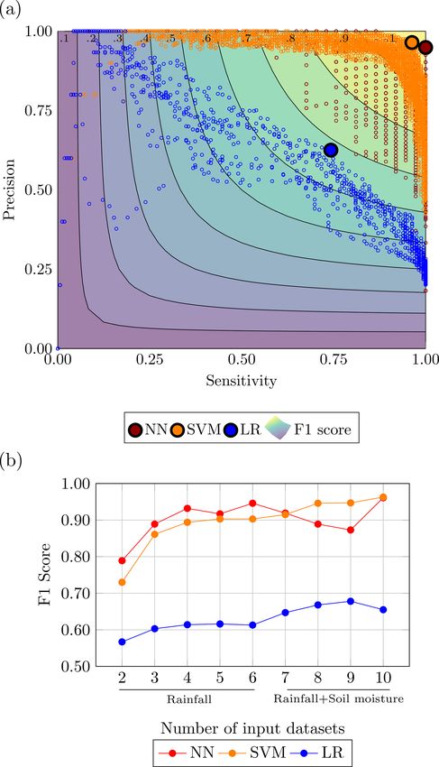
2380                                      L. Cesarini et al.: The potential of machine learning for weather index insurance

short-term liquidity gaps that may overwhelm their capac-          els used to forecast floods, while Hao et al. (2018) and Fung
ity to cope with large disasters (Van Nostrand and Nevius,         et al. (2019), in their reviews on drought forecasting, give
2011). A critical disadvantage of parametric insurance, how-       an overview of machine learning tools applied to predict
ever, is its susceptibility to basis risk, which may be defined    drought indices. Machine learning has also been employed to
as the risk that triggered payouts do not coincide with the        forecast wind gusts (Sallis et al., 2011), severe hail (Gagne
occurrence of loss events.                                         et al., 2017) and excessive rainfall (Nayak and Ghosh, 2013).
   The minimisation of basis risk in parametric insurance re-      In contrast, only a minor part of the body of literature focuses
quires a reliable, rapid and objective identification of extreme   its attention on the identification or classification of events
climate events. Nowadays, different sources of weather data        (Nayak and Ghosh, 2013, Khalaf et al., 2018, and Alipour
that may be used to support this endeavour are available.          et al., 2020, for floods; Richman et al., 2016, for droughts;
Among them, the use of satellite images and reanalyses prod-       and Kim et al., 2019 for tropical cyclones). However, clas-
ucts in parametric insurance mechanisms is growing (Black          sification of events to distinguish between extreme and non-
et al., 2016; Chantarat et al., 2013). Satellite images and re-    extreme events is essential to support the development of ef-
analyses are frequently free of charge, and therefore para-        fective parametric risk transfer instruments. In addition, the
metric models based on them are cheaper and can be afford-         major part of the analysed studies deals with a single type of
able even for developing countries (Castillo et al., 2016). In     event.
addition, satellite images and reanalyses consist of continu-         This paper aims to assess the potential of machine learning
ous spatial fields and often have global coverage. These last      for weather index insurance. To achieve this, we propose and
features make them attractive, since they overcome one of          apply a machine learning methodology that is capable of ob-
the most common issues related to gauges and weather sta-          jectively identifying extreme weather events, namely flood
tions, which is their limited or irregular spatial coverage. It    and drought, in near-real time, using quasi-global gridded
should also be noted that, hypothetically, if an entity that is    climate datasets derived from satellite imagery or a combi-
responsible for such stations (e.g. a governmental agency) is      nation of observation and satellite imagery. The focus of the
related in some form with a potential beneficiary from in-         study is then to address the following research questions.
dex insurance coverage, a conflict of interest may arise. This
                                                                    1. Can machine learning algorithms provide improvement
issue is avoided with satellite-based or reanalysis products,
                                                                       in terms of performance for weather index insurance
which are produced by third parties, for example internation-
                                                                       with respect to traditional approaches?
ally renowned research institutes such as the Climate Haz-
ards Center of the University of California and the Euro-           2. To which extent do the performances of machine learn-
pean Centre for Medium-Range Weather Forecasts. Satellite              ing models improve with the addition of input data?
images are often available with high spatial resolution, but
                                                                    3. Do the best-performing models share similar properties
records are still short, with a maximum duration of around
                                                                       (e.g. use more input data or consistently have similar
30 years. Reanalysis, on the other hand, provides longer time
                                                                       algorithm’s features)?
series but tends to have a coarser spatial resolution. More-
over, satellite data should be checked for consistency with           In this study we focus on the detection of two types of
ground measurement, which is not always feasible when the          weather events with very different features: floods, which are
network of ground instruments is inadequate or non-existent        mainly local events that can develop over a timescale going
(Loew et al., 2017). Although using satellite data has its         from few minutes to days, and droughts, which are creep-
own limitations, various index-based insurance products, ex-       ing phenomena that involve widespread areas and have a
ploiting remote-sensing data and reanalysis, have been devel-      slow onset and offset. In addition, floods cause immediate
oped in data-sparse regions such as Africa and Latin Amer-         losses (Plate, 2002), while droughts produce non-structural
ica (Awondo, 2018; African Union, 2021; The World Bank,            damages and their effects are delayed with respect to the be-
2008). The combined use of various sources of information          ginning of the event (Wilhite, 2000). Both satellite images
to detect the occurrence of extreme events is valuable, since      and reanalyses are used as input data to show the potential
it can significantly improve the ability to correctly detect ex-   of these instruments when properly designed and managed.
treme events (Chiang et al., 2007), and a proper index design      Two of the most used machine learning methodologies, neu-
helps in addressing the limitations brought by satellite data,     ral network (NN) and support vector machine (SVM), are
as underlined in Black et al. (2016).                              applied. With machine learning (ML) models it is not al-
   Over the last two decades there has been an increasing          ways straightforward to know a priori which model(s) per-
focus on the application of machine learning methods to            form(s) better or which model configuration(s) should be
process and extract information from big data with limited         used. Therefore, various model configurations are explored
human intervention (Ornella et al., 2019). Correspondingly,        for both NN and SVM, and a rigorous evaluation of their
machine learning approaches have also been applied to fore-        performances is accomplished. The best-performing config-
cast extreme events. Mosavi et al. (2018) offer an accurate        urations are tested to reproduce past extreme events in a case
description of the state of the art of machine learning mod-       study region.

Nat. Hazards Earth Syst. Sci., 21, 2379–2405, 2021                                https://doi.org/10.5194/nhess-21-2379-2021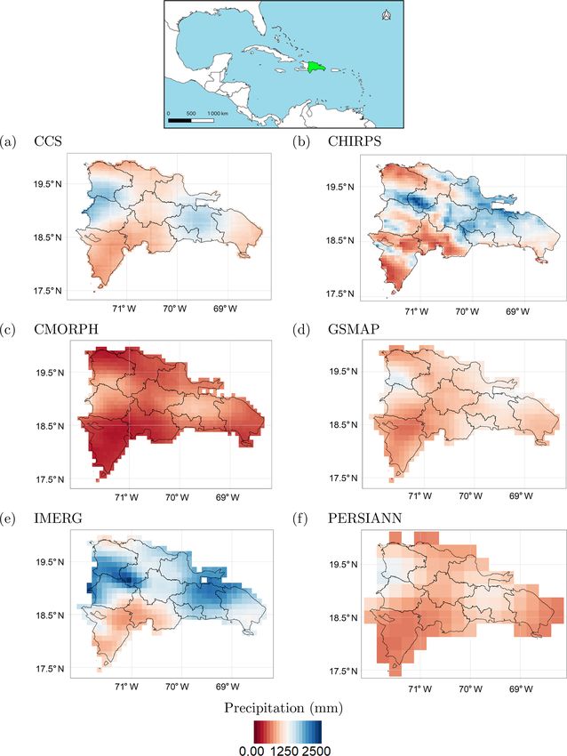
L. Cesarini et al.: The potential of machine learning for weather index insurance                                             2381

   Section 2 describes the NN and SVM algorithms used in             transformations of a set of environmental variables. This hy-
this study and their configurations, the procedure adopted to        brid approach aims to capture some of the physical processes
take into consideration the problem of data imbalance due            of how the hazard creates damage by incorporating a priori
to the rarity of extreme events, the assessment of the qual-         expert knowledge on environmental processes and damage-
ity of the classifications, and the procedure used to select         inducing mechanisms for different hazards. Raw environ-
the best-performing models and configurations. In addition,          mental variables are not always able to fully describe com-
an overview of the datasets used is provided. Section 3 pro-         plex dynamics like flood induced damage; therefore, the us-
vides some insights on the area where the described method-          age of expert knowledge is important to provide the machine
ology is applied. Section 4 presents and discusses the most          learning model with input data that are able to better charac-
important outcomes for both floods and droughts. Section 5           terise the natural hazard events.
summarises the main findings of the study, highlighting their           Supervised learning with machine learning methods based
meanings for the study case and analysing the limitations of         on physically motivated transformations of environmental
the proposed approach, while providing insight on possible           variables are then used to capture loss occurrence. The mod-
future developments.                                                 els are set up such that they produce probabilistic predic-
                                                                     tions of loss rather than directly classifying events in a bi-
                                                                     nary manner. This allows the parametric trigger to be op-
2   Methodology                                                      timised in a subsequent step, in a metrics-based, objective
                                                                     and transparent manner, by disentangling the construction
Machine learning is a subset of artificial intelligence whose
                                                                     of the model from the decision-making regarding the defini-
main purpose is to give computers the possibility to learn,
                                                                     tion of the payout-triggering threshold. Probabilistic outputs
throughout a training process, without being explicitly pro-
                                                                     are also able to provide informative predictions of loss oc-
grammed (Samuel, 1959). It is possible to distinguish ma-
                                                                     currence that convey uncertainty information, which can be
chine learning models based on the kind of algorithm that
                                                                     useful for end users when a parametric model is operational
they implement and the type of task that they are required
                                                                     (Figueiredo et al., 2018).
to solve. Algorithms may be divided into two broad groups:
                                                                        Figure 1 summarises the general framework implemented
the ones using labelled data (Maini and Sabri, 2017), also
                                                                     in this work.
known as supervised learning algorithms, and the ones that
during the training receive only input data for which the out-
                                                                     2.1   Variable and datasets selection
put variables are unknown (Ghahramani, 2004), also called
unsupervised learning algorithms.
                                                                     The data-driven nature of ML models implies that the results
   As previously mentioned, in index insurance, payouts are
                                                                     yielded are as good as the data provided. Thus, the effec-
triggered whenever measurable indices exceed predefined
                                                                     tiveness of the methods depends heavily on the choice of the
thresholds. From a machine learning perspective, this cor-
                                                                     input variables, which should be able to represent the under-
responds to an objective classification rule for predicting the
                                                                     lying physical process (Bowden et al., 2005). The data se-
occurrence of loss or no loss based on the trigger variable.
                                                                     lection (and subsequent transformation) therefore requires a
The rule can be developed using past training sets of hazard
                                                                     certain amount of a priori knowledge of the physical system
and loss data (supervised learning). Conceptually, the devel-
                                                                     under study. For the purpose of this work, precipitation and
opment of a parametric trigger should correspond to an in-
                                                                     soil moisture were used as input variables for both flood and
formed decision-making process, i.e. a process which, based
                                                                     drought. An excessive amount of rainfall is the initial trigger
on data, a priori knowledge and an appropriate modelling
                                                                     to any flood event (Barredo, 2007), while scarcity of precip-
framework, can lead to optimal decisions and effective ac-
                                                                     itation is one of the main reasons that leads to drought peri-
tions. This work aims to leverage the aptitude of machine
                                                                     ods (Tate and Gustard, 2000). Soil moisture is instead used
learning, particularly supervised learning algorithms, to sup-
                                                                     as a descriptor of the condition of the soil. With the idea to
port the decision-making process in the context of parametric
                                                                     implement a tool that can be exploited in the framework of
risk transfer, applying NN and SVM for the identification of
                                                                     parametric risk financing, we selected the datasets to retrieve
extreme weather events, namely flooding and drought for this
                                                                     the two variables according to five criteria.
particular study.
   Consider the occurrence of losses caused by a natural haz-         1. Spatial resolution. A fine spatial resolution that takes
ard on each time unit t = 1, . . ., T over a certain study area G,       into account the climatic features of the various areas
and let Lt be a binary variable defined as                               of the considered country is needed to develop accurate
                                                                         parametric insurance products.
       (
         1 if loss occurs on t in G
Lt =                                                           (1)
         0 if loss does not occur on t in G.
                                                                      2. Frequency. The selected datasets should be able to
  The aim is then to predict the occurrence of losses based              match the duration of the extreme event that we need
on a set of explanatory variables obtained from non-linear               to identify. For example, in the case of floods, which

https://doi.org/10.5194/nhess-21-2379-2021                                  Nat. Hazards Earth Syst. Sci., 21, 2379–2405, 2021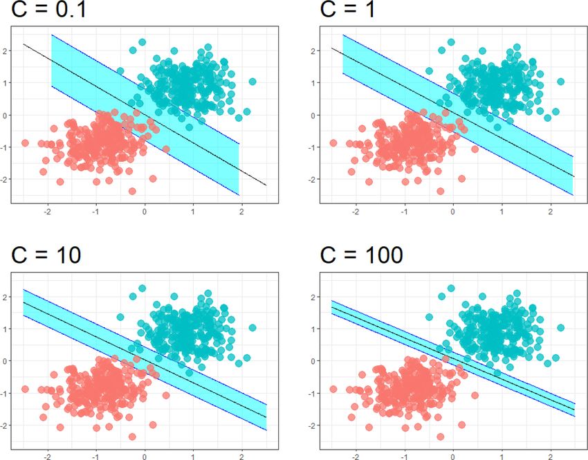
2382                                      L. Cesarini et al.: The potential of machine learning for weather index insurance

Figure 1. Flowchart of the proposed approach.

     are quick phenomena, daily or hourly frequencies are         ciated with a single variable (rainfall). The use of multiple
     required.                                                    datasets is able to improve the ability of models in identi-
                                                                  fying extreme events, as demonstrated for example by Chi-
  3. Spatial coverage. Global spatial coverage enables the        ang et al. (2007) in the case of flash floods. In addition, sin-
     extension of the developed approach to areas different       gle datasets may not perform well; the combination of vari-
     from the case study region.                                  ous datasets produces higher-quality estimates (Chen et al.,
  4. Temporal coverage. Since extreme events are rare, a          2019). Two merged satellite-gauge products (the Climate
     temporal coverage of at least 20 years is considered nec-    Hazards Group InfraRed Precipitation with Station data,
     essary to allow a correct model calibration.                 CHIRPS; and the CPC Morphing technique, CMORPH,) and
                                                                  four satellite-only (the Global Satellite Mapping of Precipi-
  5. Latency time. A short latency time (i.e. time delay to ob-   tation, GSMaP; the Integrated Multi-Satellite Retrievals for
     tain the most recent data) is necessary to develop tools     GPM, IMERG; the Precipitation Estimation from Remotely
     capable of identifying extreme events in near-real time.     Sensed Information using Artificial Neural Networks, PER-
                                                                  SIANN; and the global PERSIANN Cloud Classification
   Based on a comprehensive review of available datasets,         System, PERSIANN-CCS) datasets were used. The main
we found six rainfall datasets and one soil moisture dataset,     features of the selected datasets are reported in Table 1.
comprising four layers, matching the above criteria. With re-        Soil moisture was retrieved from the ERA5 reanalysis
spect to the studies analysed in Mosavi et al. (2018), Hao        dataset, produced by the European Centre for Medium Range
et al. (2018) and Fung et al. (2019), which associated a sin-     Weather Forecast (ECMWF). The dataset provides informa-
gle dataset to each input variable, here six datasets are asso-

Nat. Hazards Earth Syst. Sci., 21, 2379–2405, 2021                               https://doi.org/10.5194/nhess-21-2379-2021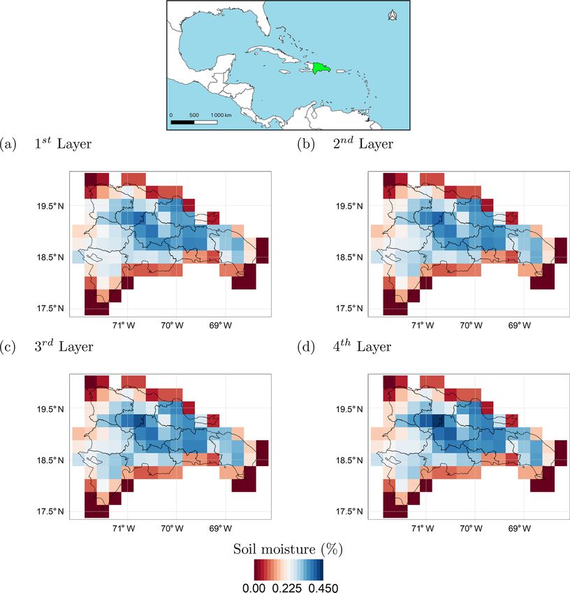
L. Cesarini et al.: The potential of machine learning for weather index insurance                                                               2383

Table 1. Main features of the selected (quasi-)global precipitation datasets.

      Dataset         Type               Resolution    Frequency   Coverage            Time span               Latency   Reference
      CCS             Satellite          0.04◦         1h          60◦ S–60◦ N         Jan 2003–present        6h        Hong et al. (2004)
      CHIRPS          Satellite gauge    0.05◦         1d          50◦ S–50◦ N         Jan 1981–present        3 weeks   Funk et al. (2015)
      CHIRP           Satellite                                                                                3d
      CMORPH          Satellite gauge    0.07◦         3h          60◦ S–60◦ N         Jan 1998–present        14 d      Joyce et al. (2004)
      GSMaP           Satellite          0.10◦         1h          60◦ S–60◦ N         Mar 2000–present        12 h      Ushio and Kachi (2010)
      IMERG           Satellite          0.10◦         30 min      60◦ S–60◦ N         Jun 2000–present        12 h      Bolvin et al. (2018)
      PERSIANN        Satellite          0.25◦         1h          60◦ S–60◦ N         Mar 2000–present        48 h      Sorooshian et al. (2000)

Table 2. Main features of the selected soil moisture dataset.

            Dataset    Type             Resolution    Frequency    Coverage      Time span                Latency     Reference
            ERA5       Reanalysis       0.25◦         1h           Global        Jan 1979–present         5d          ECMWF et al. (2018)

tion on four soil moisture layers (layer 1: 0–7 cm, layer 2:                  is restricted to a 3 d period. The potential runoff volume ac-
7–28 cm; layer 3: 28–100 cm; layer 4: 100–289 cm). Table 2                    cumulated over cell gj over days t, t − 1 and t − 2 is thus
shows the main features of the ERA5 dataset.                                  given by

2.2     Data transformation                                                   Rt∗ (gj ) = θ0 Rt (gj ) + θ1 Rt−1 (gj ) + θ2 Rt−2 (gj ),              (3)

The raw environmental variables are subjected to a trans-                     where θ0 , θ1 , θ2 > 0 and θ0 + θ1 + θ2 = 1.
formation which is dependent on the hazard at study and is                       Finally, let Yt be an explanatory variable representing po-
deemed more appropriate to enhance the performances of the                    tential flood intensity for day t, which is defined as
model, as described below.
                                                                                      J
                                                                                      X R ∗ (gj )λ − 1
                                                                                             t
2.2.1    Flood                                                                Yt =                        .                                         (4)
                                                                                      j =1
                                                                                                 λ
Flood damage is not directly caused by rainfall but from
physical actions originated by water flowing and submerg-                        The Box–Cox transformation provides a flexible, non-
ing assets usually located on land. As a result, even if floods               linear approach to convert runoff to potential damage for
are triggered by rainfall, a better predictor for the intensity of            each grid cell, which is summed over all grid cells in a study
a flood and consequent occurrence of damage is warranted.                     area to obtain a daily index of flood intensity. In order to ob-
To achieve this, we adopt a variable transformation to em-                    tain the Yt variable that best describes potential flood losses
ulate, in a simplified manner, the physical processes behind                  due to rainfall, the transformation parameters u, θ1 , θ2 and λ
the occurrence of flood damage due to rainfall, based on the                  are optimised by fitting a logistic regression model to con-
approach proposed by Figueiredo et al. (2018), which is now                   current potential flood intensity and reported occurrences of
briefly described.                                                            losses caused by flood events, as well as maximising the like-
   Let Xt (gj ) represent the rainfall amount accumulated over                lihood using a quasi-Newton method:
grid cell gj belonging to G on day t. Potential runoff is first
estimated from daily rainfall. This corresponds to the amount                 Lt ∼ Bernoulli(pt ),                                                  (5)
of rainwater that is assumed to not infiltrate the soil and thus
remain over the surface and is given by                                       with

Rt (gj ) = max{Xt (gj ) − u, 0},                                   (2)                pt
                                                                              log            = β0 + β1 Yt .                                         (6)
                                                                                    1 − pt
where u is a constant parameter that represents the daily rate
of infiltration.                                                              2.2.2     Drought
   Overland flow accumulates the excess of rainfall over the
surface of a hydrological catchment. This process is mod-                     Before being processed by the ML model, rainfall data are
elled using a weighted moving time average, which preserves                   used to compute the standardised precipitation index (SPI).
the accumulation effect and allows the contribution of rain-                  The SPI is a commonly used drought index, proposed by
fall on previous days to be considered. The moving average                    McKee et al. (1993). Based on a comparison between the

https://doi.org/10.5194/nhess-21-2379-2021                                             Nat. Hazards Earth Syst. Sci., 21, 2379–2405, 2021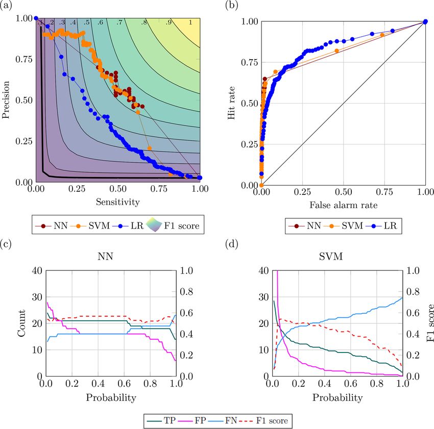
2384                                                    L. Cesarini et al.: The potential of machine learning for weather index insurance

Table 3. Drought classification based on SPI according to McKee
et al. (1993)

       Category               SPI                       Probability (%)
       Extremely wet          2.00 and above                         2.3
       Severely wet           1.50 to 1.99                           4.4
       Moderately wet         1.00 to 1.49                           9.2
       Near normal            −0.99 to 0.99                         68.2
       Moderately dry         −1.49 to −1.00                         9.2
       Severely dry           −1.50 to −1.99                         4.4
       Extremely dry          −2 and below                           2.3

long-term precipitation record (at a given location for a se-
lected accumulation period) and the observed total precipi-                       Figure 2. Learning process of a neural network (Stevens and
tation amount (for the same accumulation period), the SPI                         Antiga, 2019).
measures the precipitation anomaly. The long-term precipita-
tion record is fitted to the gamma distribution function, which
is defined according to the following equation:                                   than −1. The drought event is ongoing until SPI is up to 0
               1                                                                  (McKee et al., 1993). The main strengths of the SPI are
                              − βx
g(x) =              x α−1 e          for x > 0,                             (7)   the fact that the index is standardised, and therefore can be
         β α 0(α)
                                                                                  used to compare different climate regimes, and that it can be
where α and β are, respectively, the shape factor and the scale                   computed for various accumulation periods (World Meteo-
factor. The two parameters are estimated using the maximum                        rological Organization and Global Water Partnership, 2016).
likelihood solutions according to the following equations:                        In this study, SPI1, SPI3, SPI6 and SPI12 were computed,
         q                                                                        where the numeric values in the acronym refer to the pe-
      1 + 1 + 4D                                                                  riod of accumulation in months (e.g. SPI3 indicates the stan-
                 3
α=                 ,                                        (8)                   dard precipitation index computed over a 3-month accumula-
          4D                                                                      tion period). Shorter accumulation periods (1–3 months) are
      x
β= ,                                                        (9)                   used to detect impacts on soil moisture and on agriculture.
      α                                                                           Medium accumulation periods (3–6 months) are preferred to
where x is the mean of the distribution and N is the number                       identify reduced streamflow, and longer accumulation peri-
of observations.                                                                  ods (12–48 months) indicate reduced reservoir levels (Euro-
   The cumulative probability G(x) is defined as                                  pean Drought Observatory, 2020).

          Zx                            Zx                                        2.3     Machine learning algorithms
                          1                            − βx
G(x) =         g(x)dx = α                    x α−1 e          dx.          (10)
                       β 0(α)                                                     We now focus on the machine learning algorithms adopted in
          0                              0
                                                                                  this work, starting with a short introduction and description
   Since the gamma function is undefined if x = 0 and pre-                        of their basic functioning and next delving into the procedure
cipitation can be null, the definition of cumulative probabil-                    used to build a large number of models based on the domain
ity is adjusted to take into consideration the probability of a                   of possible configurations for each ML method. Finally, the
zero:                                                                             metrics used to evaluate the models are introduced, and the
                                                                                  reasoning behind their selection is highlighted.
H (x) = q + (1 − q)G(x),                                                   (11)

where q is the probability of a zero. H is then transformed                       2.3.1    Neural network (NN)
into the standard normal distribution to obtain the SPI value:
                                                                                  Neural networks are a machine learning algorithm composed
SPI = φ   −1
               H (x),                                                      (12)   by nodes (or neurons) that are typically organised into three
                                                                                  types of layers: input, hidden and output. Once built, a neu-
where φ is the standard normal distribution.                                      ral network is used to understand and translate the under-
   The mean SPI value is therefore zero. Negative values                          lying relationship between a set of input data (represented
indicate dry anomalies, while positive values indicate wet                        by the input layer) and the corresponding target (represented
anomalies. Table 3 reports drought classification according                       by the output layer). In recent years and with the advent of
to the SPI. Conventionally, drought starts when SPI is lower                      big data, neural networks have been increasingly used to ef-

Nat. Hazards Earth Syst. Sci., 21, 2379–2405, 2021                                                https://doi.org/10.5194/nhess-21-2379-2021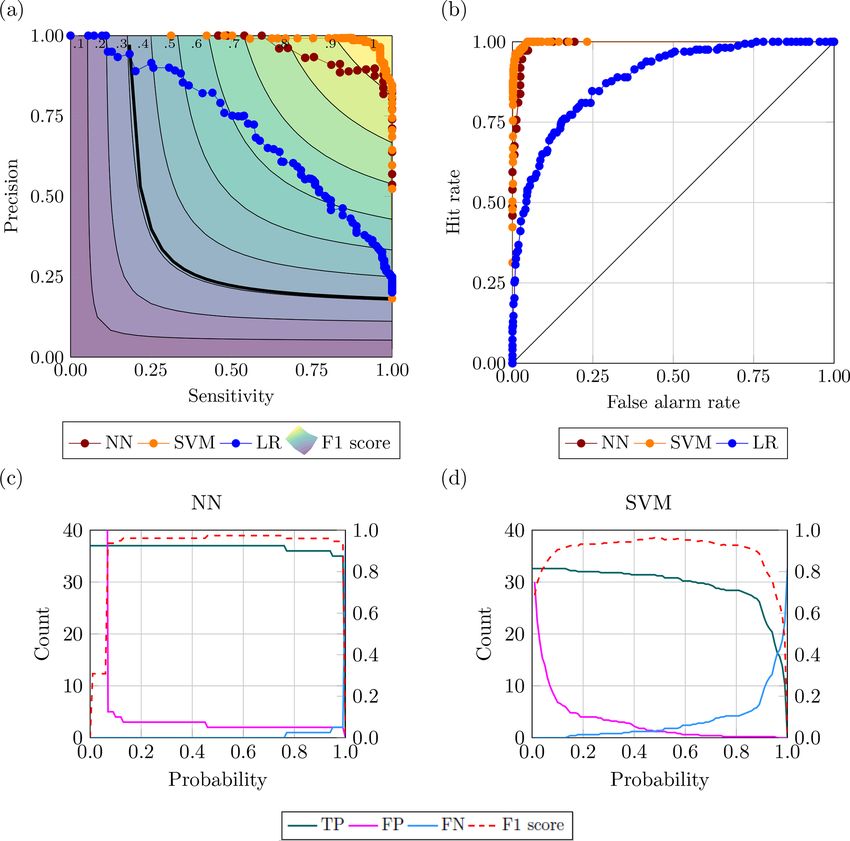
L. Cesarini et al.: The potential of machine learning for weather index insurance                                              2385

ficiently solve many real-world problems, related for exam-           Specific to the training process, monitoring the training
ple with pattern recognition and classification of satellite im-   history can provide useful information, as this graphic rep-
ages (Dreyfus, 2005), where the capacity of this algorithm         resentation of the process depicts the evolution over time of
to handle non-linearity can be put to fruition (Stevens and        the LF for both training and validation set. Looking at the
Antiga, 2019). A key problem when applying neural net-             history of the training has a twofold purpose: firstly, with
works is defining the number of hidden layers and hidden           the training being a minimisation problem, as long as the LF
nodes. This must usually be done specifically for each appli-      is decreasing the model is still learning, while any eventual
cation case, as there is no globally agreed-on procedure to de-    plateau or uprising would mean that the model is overfitting
rive the ideal configuration of the network architecture (Mas      (or not learning anymore from the data). The latter is avoided
and Flores, 2008). Although different terminology may be           when the LF of the training and validation dataset displays
used to refer to neural networks depending on their architec-      the same decreasing trend (Stevens and Antiga, 2019). The
tures (e.g, artificial neural networks, deep neural networks),     monitoring assignment is carried out during the training of
in this paper they are addressed simply as neural networks,        the model, where its capability to store the value of train-
specifying where needed the number of hidden layers and            ing and validation loss at each iteration of the process enable
hidden nodes. Figure 2 displays the different parts compos-        the possibility to stop the training as soon as losses are ei-
ing a neural network and their interaction during the learning     ther decreasing or plateauing over a certain number of itera-
process. A neural network with multiple layers can be repre-       tions. In this work, the neural network model is created and
sented as a sequence of equations, where the output of a layer     trained using TensorFlow (Abadi et al., 2016). TensorFlow is
is the input of the following layer. Each equation is a linear     an open-source machine learning library that was chosen for
transformation of the input data, multiplied by a weight (w)       this work due to its flexibility, the capacity to exploit GPU
and the addition of a bias (b) to which a fixed non-linear func-   cards to ease computational costs, its ability to represent a
tion is applied (also called activation function):                 variety of algorithms and most importantly the possibility to
                                                                   carefully evaluate the training of the model.
x1 = f (w0 x0 + b0 )
x2 = f (w1 x1 + b1 )
  ..
   .                                                               2.3.2   Support vector machine (SVM)
y = f (wn xn + bn ).                                       (13)

   The goal of these equations is to diminish the difference
between the predicted output and the real output. This is at-      The support vector machine is a supervised learning algo-
tained by minimising a so-called loss function (LF) through        rithm used mainly for classification analysis. It construct a
the fine-tuning of the parameters of the model, the weights.       hyperplane (or set of hyperplanes) defining a decision bound-
The latter procedure is carried out by an optimiser, whose         ary between various data points representing observations in
job is to update the weights of the network based on the error     a multidimensional space. The aim is to create a hyperplane
returned by the LF.                                                that separates the data on either side as homogeneously as
   The iterative learning process can be summarised by the         possible. Among all possible hyperplanes, the one that cre-
following steps:                                                   ates the greatest separation between classes is selected. The
                                                                   support vectors are the points from each class that are the
 1. start the network with random weights and bias;                closest to the hyperplane (Wang, 2005). In parametric trigger
                                                                   modelling, as in many other real-world applications, the rela-
 2. pass the input data and obtain a prediction;                   tionships between variables are non-linear. A key feature of
                                                                   this technique is its ability to efficiently map the observations
 3. compare the prediction with the real output and compute        into a higher-dimension space by using the so-called kernel
    the LF, which is the function that the learning process is     trick. As a result, a non-linear relationship may be trans-
    trying to minimise;                                            formed into a linear one. A support vector machine can also
                                                                   be used to produce probabilistic predictions. This is achieved
 4. backpropagate the error, updating each parameter               by using an appropriate method such as Platt scaling (Platt,
    through an optimiser according to the LF;                      1999), which transforms its output into a probability distri-
                                                                   bution over classes by fitting a logistic regression model to a
 5. iterate the previous step until the model is trained prop-     classifier’s scores. In this work, the support vector machine
    erly – this is achieved by stopping the training process       algorithm was implemented using the C-support vector clas-
    either when the LF is not decreasing anymore or when           sification (Boser et al., 1992) formulation implemented with
    a monitored metric has stopped improving over a set            the scikit-learn package in Python (Pedregosa et al., 2011).
    amount of definition.                                          Given training vectors xi ∈ R p i = i, . . ., l and a label vector

https://doi.org/10.5194/nhess-21-2379-2021                                 Nat. Hazards Earth Syst. Sci., 21, 2379–2405, 2021
2386 L. Cesarini et al.: The potential of machine learning for weather index insurance
Figure 3. Decision boundary of the support vector machine’s algorithm, with changing regularisation parameter C.
y ∈ {0, 1}n , this specific formulation is aimed at solving the the steps followed in order to create the best-performing NN
following optimisation problem: and SVM models from the focus placed on the importance
of data enhancing to the selection of appropriate evaluation
l metrics, exploring as many model configuration as possible,
1 X
being aware of the several parameters comprising these mod-
min(w, b, ξ ) = ωt ω + C ξi
2 i=1 els and the wide ranges that these parameters can have.
subject to y1 (ωt 9(xi ) + b) ≥ 1 − ξi
Preprocessing of data
ξi ≥ 0, i = 1, . . ., l, (14)
where ω and b are adjustable parameters of the function gen- Data preprocessing (DPP) is a vital step to any ML under-
erating the decision boundary, 9i is a function that projects taking, as the application of techniques aimed at improving
xi into a higher dimensional space, ξi is the slack variable and the quality of the data before training leads to improvement
C > 0 is a regularisation parameter, which regulates the mar- of the accuracy of the models (Crone et al., 2006). Moreover,
gin of the decision boundary, allowing an increasing number data preprocessing usually results in smaller and more reli-
of misclassifications for a lower value of C and a decreasing able datasets, boosting the efficiency of the ML algorithm
number of misclassifications for higher C (Fig. 3). (Zhang et al., 2003). The literature presents several opera-
tions that can be adopted to transform the data depending on
2.3.3 Model construction the type of task the model is required to carry out (Huang
et al., 2015; Felix and Lee, 2019). In this paper, preprocess-
Below a procedure to assemble the machine learning models ing operations were split into four categories: data quality
is proposed, which involves techniques borrowed from the assessment, data partitioning, feature scaling and resampling
data mining field and a deep understanding of all the com- techniques aimed at dealing with class imbalance. The first
ponents of the algorithms. The main purpose is to identify three are crucial for the development of a valid model, while
the actions required to establish a robust chain of model con- the latter is required when dealing with the classification of
struction. Hypothetically speaking, one may create a neural rare events. Data quality assessment was carried out to en-
network with an infinite number of layers or a support vec- sure the validity of the input data, filtering out any anomalous
tor machine model with infinite values of the C regularisa- value (e.g. negative values of rainfall).
tion parameters. Figure 4, an expanded diagram of the ML The partitioning of the dataset into training, validation and
algorithm box of the workflow shown in Fig. 1, describes testing portions is fundamental to give the model the ability
Nat. Hazards Earth Syst. Sci., 21, 2379–2405, 2021 https://doi.org/10.5194/nhess-21-2379-2021L. Cesarini et al.: The potential of machine learning for weather index insurance 2387
set that the model has never seen. Concerning the SVMs, a
k-fold cross validation (Mosteller and Tukey, 1968) was used
to validate the model, using 5 folds created by preserving the
percentage of sample of each class; the algorithm was there-
fore trained on 80 % of the data and its performances were
evaluated on 20 % of the remaining data that the model had
never seen.
Feature scaling is a procedure aimed at improving the
quality of the data by scaling and normalising numeric val-
ues so as to help the ML model in handling varying data in
magnitude or unit (Aksoy and Haralick, 2001). The variables
are usually rescaled to the [0, 1] range or to the [−1, 1] range
or normalised subtracting the mean and dividing by the stan-
dard deviation. The scaling is carried on after the splitting of
the data and is usually calibrated over the training data, and
then the testing set is scaled with the mean and variance of
the training variables (Massaron and Muller, 2016).
Lastly, when undertaking a classification task, particular
attention should be paid to addressing class imbalance, which
reflects an unequal distribution of classes within a dataset.
Imbalance means that the number of data points available
for different classes is significantly different; if there are two
classes, a balanced dataset would have approximately 50 %
points for each of the classes. For most machine learning
techniques, a little imbalance is not a problem, but when the
class imbalance is high, e.g. 85 % points for one class and
15 % for the other, standard optimisation criteria or perfor-
Figure 4. Framework used to analyse the domain of possible model mance measures may not be as effective as expected (Garcia
configurations. et al., 2012). Extreme events are by definition rare; hence,
the imbalance existing in the dataset should be addressed.
One approach to address imbalances is using resampling
to learn from the data and avoid a problem often encountered techniques such as oversampling (Ling and Li, 1998) and
in ML application: overfitting. This phenomenon takes place SMOTE (Chawla et al., 2002). Oversampling is the pro-
when a model starts overlearning from the training dataset, cess of up-sampling the minority class by randomly duplicat-
picking up patterns that belong solely to the specific set of ing its elements. SMOTE (Synthetic Minority Oversampling
data it is training on and that are not depictive of the real- Technique) involves the synthetic generation of data looking
world application at hand, making the model unable to gen- at the feature space for the minority class data points and con-
eralise to sample outside this specific set of data. To avoid sidering its k nearest neighbour where k is the desired num-
overfitting one should split the data into at least two parts ber of synthetic generated data. Another possible approach to
(McClure, 2017): the training set, upon which the model will address imbalances is weight balancing, which restores bal-
learn, and a validation dataset functioning as a counterpart ance in the data by altering the way the model “looks” at the
during the training process of the model, where the losses under-represented class. Oversampling, SMOTE and class
obtained from the training set and those obtained from the weight balancing were the resampling techniques deemed
validation set are compared to avoid overfitting. A further more appropriate to the scope of this work, namely, identi-
step would be to set aside a testing set of data that the model fying events in the minority class.
has never seen. Evaluating the performances of the model
using data that it has never encountered before is an excel- Analysis of model configurations
lent indicator of its ability to generalise. Thus, the splitting
of the data is key to the validation of the model. In this work, Up to this point, several models characteristics and a consid-
the training of the NN was carried out splitting the dataset erable amount of possible operations aimed at data augmen-
into three parts: training (60 %), validation (15 %) and test- tation were presented, creating an almost boundless domain
ing (25 %) sets. During training, the neural networks used of model configurations. In order to explore such a domain,
only the training set, evaluating the loss on the validation set for each ML method multiple key aspects were tested. Both
at each iteration of the training process. After the training, methods shared an initial investigation of the sampling tech-
the performance of the model was evaluated on the testing nique and the combination of input datasets to be fed into the
https://doi.org/10.5194/nhess-21-2379-2021 Nat. Hazards Earth Syst. Sci., 21, 2379–2405, 20212388 L. Cesarini et al.: The potential of machine learning for weather index insurance
models; all the data resampling techniques previously intro- the matrix (e.g. high precision may be achieved by a model
duced were tested along with the data in their pristine con- that is predicting a high value of false negatives). Nonethe-
dition where the model tries to overcome the class imbal- less, they are staples in the evaluation of binary classifica-
ance by itself. All the possible combinations of input dataset tion, providing insightful information depending on the prob-
were tested starting from one dataset for SVM and with two lem addressed. Accuracy and F1 score, on the other hand,
datasets for NN up to the maximum number of environmen- are obtained by considering both directions of the confu-
tal variables used. The latter procedure can be used to deter- sion matrix, thus giving a score that incorporates both cor-
mine whether the addition of new information is beneficial rect predictions and misclassifications. The accuracy is the
to the predictive skill of the model and also to identify which ratio between the correct prediction over all the instances of
datasets provide the most relevant information. the dataset and is able to tell how often, overall, a model is
As previously discussed, these models present a multitude correct. The F1 score is the harmonic mean of precision and
of customisable facets and parameters. For the support vector recall. In its general formulation derived from the effective-
machine, the regularisation parameter C and the kernel type ness measure of Jones and Van Rijsbergen (1976), one may
were the elements chosen as the changing parts of the algo- define a Fβ score for any positive real β (Eq. 15):
rithm. Five different values of C were adopted, starting from
precision · sensitivity
a soft margin of the decision boundary moving towards nar- Fβ = 1 + β 2 , (15)
rower margins, while three kinds of kernel functions were (β 2 · precision) + sensitivity
used to find the separating hyperplane: linear, polynomial where β denotes the importance assigned to precision and
and radial. The setup for a neural network is more complex sensitivity. In the F1 score both are considered to have the
and requires the involvement of more parameters, namely, same weight. For values of β higher than 1 more significance
the LF and the optimisers concerning the training process, is given to false negatives, while β lower than 1 puts attention
plus the number of layers and nodes and the activation func- on the false positive.
tions as key building blocks of the model architecture. Each The goodness of a model may also be assessed in broader
of the aforementioned parameters can be chosen among a terms with the aid of receiver operating characteristic (ROC)
wide range of options; moreover, there is not a clear indi- and precision-sensitivity curves (PS). The ROC curve is
cation for the number of hidden layers or hidden nodes that widely employed and is obtained by plotting the sensitivity
should be used for a given problem. Thus, for the purpose of against the false alarm rate over the range of possible trig-
this study, the intention was to start from what was deemed ger thresholds (Krzanowski and Hand, 2009). The PS curve,
the “standard” for the classification task for each of these pa- as the name suggests, is obtained by plotting the precision
rameters, deviating from these standard criteria towards more against the sensitivity over the range of possible thresholds.
niche instances of the parameters trying to cover as much as For this work, the threshold corresponds to the range of prob-
possible of the entire domain. abilities between 0 and 1. These methods allow for evaluating
a model in terms of its overall performance over the range
2.4 Evaluation of predictive performance of probabilities, by calculating the so-called area under the
curve (AUC). It should be noted that both the ROC curve
The evaluation of the predictive performance of the mod- and the accuracy metric should be used with caution when
els is fundamental to select the best configuration within the class imbalance is involved (Saito and Rehmsmeier, 2015),
entire realm of possible configurations. A reliable tool to as having a large amount of true negative tends to result in a
objectively measure the differences between model outputs low false-positive-rate value (FPR = 1 − specificity). Table 5
and observations is the confusion matrix. Table 4 shows a summarises the metrics described above used in this paper to
schematic confusion matrix for a binary classification case. evaluate model performances.
When dealing with thousands of configurations and, for each In the context of performance evaluation, it is also rele-
configuration, with an associated range of possible threshold vant to discuss how class imbalance might affect measures
probabilities, it is impracticable to manually check a table or that use the true negative in their computation. Saito and
a graph for each setup of the model. Therefore, a numeric Rehmsmeier (2015) tested several metrics on datasets with
value, also called evaluation metric, is often employed to varying class imbalance and showed how accuracy, sensi-
synthesise the information provided by the confusion matrix tivity and specificity are insensitive to the class imbalance.
and describe the capability of a model (Hossin and Sulaiman, This kind of behaviour from a metric can be dangerous and
2015). definitely misleading when assessing the performances of a
There are basic measures that are obtained from the pre- ML algorithm and might lead to the selection of a poorly
dictions of the model for a single threshold value (i.e. value designed model (Sun et al., 2009), emphasising the impor-
above which an event is considered to occur). These in- tance of using multiple metrics when analysing model perfor-
clude the precision, sensitivity, specificity and false alarm mances. Lastly, once the domain of all configurations was es-
rate, which take into consideration only one row or column tablished and the best settings of the ML algorithms were se-
of the confusion matrix, thus overlooking other elements of lected based on the highest values of F1 score and area under
Nat. Hazards Earth Syst. Sci., 21, 2379–2405, 2021 https://doi.org/10.5194/nhess-21-2379-2021L. Cesarini et al.: The potential of machine learning for weather index insurance 2389
Table 4. Contingency table for the deterministic estimates of a series of binary events.
Event observed
Event predicted Yes No Total
Yes a (true positive) b (false positive) a+b
No c (false negative) d (true negative) c+d
Total a+c b+d a+b+c+d = n
Figure 5. Average annual rainfall over the Dominican Republic according to the six considered datasets. (a) CCS, (b) CHIRPS, (c) CMORPH,
(d) IMERG, (e) GSMaP and (f) PERSIANN.
https://doi.org/10.5194/nhess-21-2379-2021 Nat. Hazards Earth Syst. Sci., 21, 2379–2405, 20212390 L. Cesarini et al.: The potential of machine learning for weather index insurance
Table 5. Key metrics for the evaluation of model performance; a, b, are considered. It is interesting to note that all the datasets
c and d are defined in Table 4. show similar precipitation patterns; on average, over the pe-
riod from 2000 to 2019, rainfall was mainly concentrated in
Metric Equation north-western regions, along the Haitian borders, with the
Accuracy (a + d)/n south-western regions being the driest. The situation is dif-
Precision a/(a + b) ferent when considering the average soil moisture (Fig. 6).
Sensitivity (recall) a/(a + c) The central regions are the wettest, while the driest areas
False alarm rate b/(b + d) are located on the coast. There are no significant differences
precision·sensitivity
F1 score 2 · precision+sensitivity among the four soil moisture layers.
R1
AUC under the ROC curve ROC(t)dt Weather-related disasters have a significant impact on the
R01 economy of the Dominican Republic. The country is ranked
AUC under the PS curve 0 PS(t)dt
as the 10th most vulnerable in the world and the second in
the Caribbean, as per the Climate Risk Index for 1997–2016
report (Eckstein et al., 2017). It has been affected by spatial
the PS curve, the predictive performances of the models were
and temporal changes in precipitation, sea level rise, and in-
compared to those of logistic regression (LR) models. The
creased intensity and frequency of extreme weather events.
logistic regression adopted as a baseline takes as input mul-
Climate events such as droughts and floods have had signif-
tiple environmental variables, in line with the procedure fol-
icant impacts on all the sectors of the country’s economy,
lowed for the ML methods, and used a logit function (Eq. 6)
resulting in socio-economic consequences and food insecu-
as a link function, neglecting interaction and non-linear ef-
rity for the country. According to the International Disaster
fects amid predictors. The logistic regression is a more tradi-
Database EMDAT (CRED, 2019), over the period from 1960
tional statistical model whose application to index insurance
to present, the most frequent natural disasters were tropical
has recently been proposed and can be said to already rep-
cyclones (45 % of the total natural disasters that hit the coun-
resent in itself an improvement over common practice in the
try), followed by floods (37 %) . Floods, storms and droughts
field (Calvet et al., 2017; Figueiredo et al., 2018). Thus, this
were the disasters that affected the largest number of people
comparison is able to provide an idea about the overall ad-
and caused huge economic losses.
vantages of using a ML method.
The performances of a ML model are strictly related to the
data the algorithm is trained on; hence, the reconstruction of
3 Case study historical events (i.e. the targets), although time-consuming,
is paramount to achieve solid results. Therefore, a wide range
This study adopts the Dominican Republic as its case study. of text-based documents from multiple sources have been
The Dominican Republic is located on the eastern part of consulted to retrieve information on past floods and droughts
the island of Hispaniola, one of the Greater Antilles, in the that hit the Dominican Republic over the period from 2000
Caribbean region. Its area is approximatively 48 671 km2 . to 2019. International disasters databases, such as the world-
The central and western parts of the county are mountain- renowned EMDAT, Desinventar and ReliefWeb, have been
ous, while extensive lowlands dominate the south-east (Izzo considered as primary sources. The events reported by the
et al., 2010). datasets have been compared with the ones present in hazard-
The climate of the Dominican Republic is classified as specific datasets (such as FloodList and the Dartmouth Flood
“tropical rainforest”. However, due to its topography, the Observatory) and in specific literature (Payano-Almanzar
country’s climate shows considerable variations over short and Rodriguez, 2018; Herrera and Ault, 2017) to produce a
distances. The average annual temperature is about 25 ◦ C, reliable catalogue of historical events. Only events reported
with January being the coldest month (average monthly tem- by more than one source were included in the catalogue. Fig-
perature over the period 1901–2009 of about 22 ◦ C) and Au- ure 7 shows the past floods and droughts hitting the Domini-
gust the hottest (average monthly temperature over the pe- can Republic over the period from 2000 to 2019. More de-
riod 1901–2009 of about 26 ◦ C) (World Bank, 2019). Rain- tails on the events can be found in Tables A1 (floods) and A2
fall varies from 700 to 2400 mm yr−1 , depending on the re- (droughts).
gion (Payano-Almanzar and Rodriguez, 2018). The six con-
sidered rainfall datasets (described in Table 1) exhibit con-
siderable differences in average annual precipitation values 4 Results and discussion
over the Dominican Republic (Fig. 5), with CMORPH show-
ing the lowest values and CHIRPS and IMERG the highest The results are presented in this section separating the two
ones. Nevertheless, the difference among absolute precipi- types of extreme events investigated, flood and drought. As
tation values does not affect the results of this study since described in Sect. 2, both NN and SVM models require the
precipitation is transformed into potential damage or SPI, as assembling of several components. Table 6 collects the num-
described in Sect. 2.2.2, and therefore only relative values ber of model configurations explored, broken down by type
Nat. Hazards Earth Syst. Sci., 21, 2379–2405, 2021 https://doi.org/10.5194/nhess-21-2379-2021L. Cesarini et al.: The potential of machine learning for weather index insurance 2391
Figure 6. Average soil moisture over the Dominican Republic in the four soil moisture layers. (a) First layer, 0–7 cm; (b) second layer,
7–28 cm; (c) third layer, 28–100 cm; (d) fourth layer, 100–289 cm.
Figure 7. Overview of floods and droughts hitting the Dominican Republic over the period 2000–2019.
of hazard and ML algorithm with their respective parameters. 2. the remaining combinations are obtained adding pro-
The main differences between the ML models parameters for gressively layers of soil moisture to the ensemble of six
the two hazards reside in which data are provided to the algo- rainfall datasets;
rithm and which sampling techniques are adopted. The input
dataset combination were chosen as follows: 3. the drought case required the investigation of the SPI
over different accumulation periods, and 1-, 3-, 6- and
12-month SPI values were used.
1. all the possible combinations from one up to six rainfall Neural networks and support vector machines alike are
datasets (for neural networks two rainfall datasets were able to return predictions (i.e. outputs) as a probability when
considered the starting point); the activation function allows it (e.g. sigmoid function), en-
https://doi.org/10.5194/nhess-21-2379-2021 Nat. Hazards Earth Syst. Sci., 21, 2379–2405, 20212392 L. Cesarini et al.: The potential of machine learning for weather index insurance
Table 6. Breakdown of all the configuration explored by algorithm and type of hazard.
Model Parameter Flood Drought
Input dataset combinations 61 combinations of environmental variables 61 combinations of environmental variables
4 SPI (1,3,6,12)
Sampling Unweighted Unweighted
Class weight Class weight
Oversampling
NN SMOTE
Loss Binary cross entropy Binary cross entropy
Optimiser ADAM ADAM
Number of layers & nodes Layers: [1; 9] Layers: [1; 9]
Nodes: 2nl+1 : 2nl+9 (∗) Nodes 2nl+1 : 2nl+9 (∗)
Activations ReLU ReLU
Tanh Tanh
Number of configurations 4392 8784
SVM Input dataset combinations 67 combinations of environmental variables 67 combinations of environmental variables
4 SPI (1,3,6,12)
Sampling technique Unweighted Unweighted
Class weight Class weight
Oversampling
SMOTE
C regularisation parameter C = (0.1, 1, 10, 100, 500) C = (0.1, 1, 10, 100, 500)
Kernel function Linear Linear
Polynomial Polynomial
Radial basis Radial basis
Number of configurations 4020 8040
∗ nl: number of layers.
Figure 8. Comparison of the predictions of the three methods over the testing set vs. the observed events. Flood case.
abling the possibility to find an optimal value of probabil- best-performing model configurations for the whole range
ity to assess the quality of the predictions . Therefore, for of probabilities according to the AUC of the precision-
each hazard, the results are presented by introducing at first sensitivity curve are presented and discussed. The reasoning
the models achieving the highest value of the F1 score for behind the selection of these metrics is discussed in Sect. 2.4.
a given configuration and threshold probability (i.e. a point As described in the same section, the performances of the
in the ROC or precision-sensitivity space). Secondly, the
Nat. Hazards Earth Syst. Sci., 21, 2379–2405, 2021 https://doi.org/10.5194/nhess-21-2379-2021L. Cesarini et al.: The potential of machine learning for weather index insurance 2393
oversampling to the input data. The network architecture was
made up of nine hidden layers with the number of nodes for
each layer as already described, activated by a ReLU func-
tion. The LF adopted was the binary cross entropy, and the
weights update was regulated by an Adam optimiser. The
highest F1 score for the support vector machine was attained
by the model configuration using an unweighted model tak-
ing advantage of all 10 environmental variables with a radial
basis function as kernel type and a C parameter equal to 500
(i.e. harder margin). Figure 8 shows the predictions of the
two machine learning models and the baseline logistic re-
gression, as well as the observed events. The corresponding
evaluation metrics are summarised in Table 7, which refer to
results measured on the testing set and, therefore, never seen
by the model. Overall, the two ML methods outperform de-
cisively the logistic regression with a slightly higher F1 score
for the neural network.
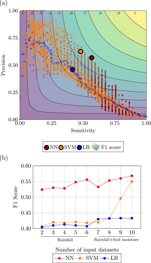
In Fig. 9a the highest F1 scores by method are reported in
the precision-sensitivity space along with all the points be-
longing to the top 1 % configurations according to F1 score.
The separation between the ML methods and the logistic re-
gression can be appreciated, particularly when looking at the
emboldened dots in Fig. 9 representing the highest F1 score
for each method. Also, the plot highlights a denser cloud of
orange points in the upper left corner and a denser cloud of
red points in the lower right corner, attesting, on average, a
higher sensitivity achieved by the NNs and a higher precision
by the SVMs.
Figure 9b depicts the goodness of NN and SVM vs. the LR
model, showing how the F1 scores of the best-performing
settings for each of the three methods vary by increasing
the number of input datasets. This plot shows that the SVM
and LR models have similar performances up to the sec-
ond layer of soil moisture, while NN performs considerably
better overall. The NN and the SVM as opposed to the LR
Figure 9. Performance evaluation for the flood case: (a) perfor- show an increase in the performances of the models with in-
mances of the top 1 % configurations in the precision-sensitivity creasing information provided. The LR seems to plateau af-
space highlighting the highest F1 score and (b) comparison of ML ter four rainfall datasets, and the improvements are minimal
methods with LR with combination using increasing number of in- after the first layer of soil moisture is fed to the model. This
put datasets. would suggest, as expected, that the ML algorithms are better
equipped to treat larger amounts of data.
Figure 10 presents the best-performing configurations ac-
ML algorithms are evaluated through a comparison with a cording to the area under the PS curve. For neural network,
LR model. this configuration is the one that also contains the highest
F1 score, whereas for support vector machine the optimal
4.1 Flooding configuration shares the same feature of the one with the
best F1 score with the exception of a softer decision bound-
The flood case presented a strong challenge from the data ary in the form of C equal to 100. The results reported in
point of view. Inspecting the historical catalogue of events Fig. 10a and b about the best-performing configurations are
the case study reported 5516 d with no flood events occur- further confirmation of the importance of picking the right
ring and 156 d of flood, meaning approximately a 35 : 1 ratio compound measurement to evaluate the predictive skill of a
of no event / event. This strong imbalance required the use model. In fact, according to the metrics using the true nega-
of the data augmentation techniques presented in Sect. 2.3.1. tive in their computation (i.e. specificity, accuracy and ROC),
The neural network settings returning the highest F1 score one may think that these models are rather good, and this
were given by the model using all 10 datasets applying an deceitful behaviour is not scaled appropriately for very bad
https://doi.org/10.5194/nhess-21-2379-2021 Nat. Hazards Earth Syst. Sci., 21, 2379–2405, 2021You can also read