Applications of Artificial Neural Networks in Microorganism Image Analysis: A Comprehensive Review from Conventional Multilayer Perceptron to ...
←
→
Page content transcription
If your browser does not render page correctly, please read the page content below
Noname manuscript No.
                                        (will be inserted by the editor)

                                        Applications of Artificial Neural Networks in
                                        Microorganism Image Analysis: A Comprehensive
                                        Review from Conventional Multilayer Perceptron
                                        to Popular Convolutional Neural Network and
                                        Potential Visual Transformer

                                        Jinghua Zhang1,2 · Chen Li1,∗,# · Marcin
                                        Grzegorzek2
                                        Received: date / Accepted: date
arXiv:2108.00358v1 [cs.CV] 1 Aug 2021

                                        Abstract Microorganisms are widely distributed in the human daily living
                                        environment. They play an essential role in environmental pollution control,
                                        disease prevention and treatment, and food and drug production. The identifi-
                                        cation, counting, and detection are the basic steps for making full use of differ-
                                        ent microorganisms. However, the conventional analysis methods are expen-
                                        sive, laborious, and time-consuming. To overcome these limitations, artificial
                                        neural networks are applied for microorganism image analysis. We conduct
                                        this review to understand the development process of microorganism image
                                        analysis based on artificial neural networks. In this review, the background
                                        and motivation are introduced first. Then, the development of artificial neural
                                        networks and representative networks are introduced. After that, the papers
                                        related to microorganism image analysis based on classical and deep neural
                                        networks are reviewed from the perspectives of different tasks. In the end, the
                                        methodology analysis and potential direction are discussed.
                                        Keywords Microorganism image analysis · Classical neural network · Deep
                                        neural network · Transfer learning

                                        1 Introduction

                                        Microorganisms are tiny living organisms that can appear as unicellular, multi-
                                        cellular, and acellular types [91]. We provide some examples in Fig. 1. Some mi-
                                        croorganisms are benefiting, such as Lactobacteria can decompose substances
                                        to give nutrients to plants [70], Actinophrys can digest the organic waste in

                                        1. Microscopic Image and Medical Image Analysis Group, College of Medicine and Biological
                                        Information Engineering, Northeastern University, Shenyang, China
                                        2. Institute for Medical Informatics, University of Luebeck, Luebeck, Germany
                                        ∗. Co-first author: Chen Li
                                        #. Corresponding author: Chen Li, E-mail: lichen201096@hotmail.com; Marcin Grzegorzek,
                                        E-mail: marcin.grzegorzek@uni-luebeck.de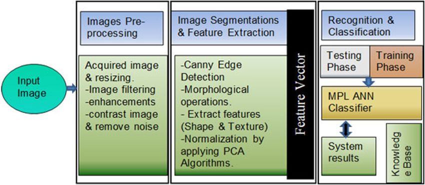
2                                                                 Jinghua Zhang1,2 et al.

sludge and increase the quality of freshwater [167], and Rhizobium legumi-
nosarum can help soybean to fix nitrogen and supply food to human beings [8].
However, there are also many harmful microorganisms, such as Mycobacterium
tuberculosis can lead to disease and death [43], and the novel coronavirus dis-
ease 2019 (COVID-19) constitutes a public health emergency globally [112].
Therefore, microorganism research plays a vital role in pollution monitoring,
environmental management, medical diagnosis, agriculture, and food produc-
tion [70, 80], and the analysis of microorganisms is the essential step for related
researches and applications [82].

    Actinophrys   Arcella     Aspidisca    Codosiga    Colpoda     Epistylis     Euglypha

    Paramecium    Rotifera    Vorticella   Noctiluca   Ceratium    Stentor      Siprostomum

    K.Quadrala    Euglena    Gymnodinium   Gonyaulax   Phacus     Stylonychia    Synchaeta

Fig. 1 The examples of images of the investigated classes of microorganisms [167].

    In general, microorganism analysis methods can be summarised into four
categories: chemical (e.g., chemical component analysis), physical (e.g., spec-
trum analysis), molecular biological (e.g., DNA and RNA analysis), and mor-
phological (e.g.manual observation under a microscope) methods [80]. Their
main advantages and disadvantages are compared in Table 1. The chemical
method is highly accurate but often results in secondary pollution of chemical
reagent [80]. The physical method also has high accuracy, but it requires expen-
sive pieces of equipment [80]. The molecular biological method distinguishes
microorganism by sequence analysis of genome [159]. This strategy needs ex-
pensive pieces of equipment, plenty of time, and professional researchers. The
morphological method is the most direct and brief approach, where a microor-
ganism is observed under a microscope and recognized manually based on its
shape [106]. The morphological method is the most cost-effective of the above
methods, but it is still laborious, tedious, and time-consuming [167]. Besides,
the objectivity of this manual analyzing process is unstable, depending on the
experience, workload, and mood of the biologist significantly.
    In recent years, Artificial Intelligence (AI) technology develops rapidly [169].
It achieves outstanding performance in many fields of image analysis and pro-
cessing, such as autonomous driving [125, 18, 147], face recognition [88, 146,
32], and disease diagnosis [133, 83, 112]. AI can undertake the laborious and
Title Suppressed Due to Excessive Length                                                   3

Table 1 A comparison of traditional methods for microorganism analysis [77].

        Methods             Advantages                     Disadvantages
    Chemical method         High accuracy      Secondary pollution of chemical reagent
    Physical method         High accuracy               Expensive equipment
   Molecular biological                        Secondary pollution of chemical reagent,
                            High accuracy
         method                                expensive equipment, long testing time
  Morphological method    Short testing time   Long training time for skillful operators

time-consuming work and quickly extract valuable information from image
data. Therefore, AI shows potential in Microorganism Image Analysis (MIA).
Besides, AI has a strong objective analysis ability in MIA and can avoid subjec-
tive differences caused by manual analysis. To some extent, the misjudgement
of biologists can be reduced, and the efficiency can be improved.
    As an essential part of artificial intelligence technology, Artificial Neural
Network (ANN) is originally designed according to the biological neuron [93].
Due to the limitation of computer performance, the difficulty of training, and
the popularization of Support Vector Machine (SVM), the early ANN devel-
opment once fall into a state of stagnation [160]. After that, with the improve-
ment of computer performance, Convolutional Neural Network (CNN) shows
an overwhelming advantage in image recognition [68], and ANN is paid at-
tention to again and developed rapidly. We find that ANNs are widely used
in MIA thorough investigation because they can learn useful patterns from
enormous data and features.

1.1 Artificial Intelligence Methods for Microorganism Image Analysis

AI is an umbrella term encompassing the techniques for a machine to mimic or
go beyond human intelligence, primarily in cognitive capabilities [116]. Fig. 2
provides the structure of AI technology [86, 169]. AI has several important sub-
domains, such as Machine learning (ML), computer vision, natural language
processing, etc. Among them, ML technology has been widely used in the
MIA task, such as Environmental Microorganism (EM) segmentation [82, 167],
Herpesvirus detection [33], and Tuberculosis Bacilli (TB) classification [121,
103].
    As shown in Fig. 2, ML can be grouped into conventional methods and
ANNs. In conventional methods, SVM, k-Nearest Neighbor (KNN), Random
Forest (RF) and other methods have been applied to the MIA task. For ex-
ample, work [79] proposes an automatic EM classification system based on
content-based image analysis techniques. There are four features (histogram
descriptor, geometric feature, Fourier descriptor and internal structure his-
togram) extracted from the Sobel edge detector based segmentation result for
training SVM to perform the classification task. For ten EM classes tested in
4                                                                                                      Jinghua Zhang1,2 et al.

                                                               Artificial
                                                             Intelligence

                           Natural
    Computer                                    Speech        Machine                 Expert
                          Language                                                                          Robotics
     Vision                                   Recognition     Learning                System
                          Processing

                                                                                               Artificial
                        Conventional
                                                                                                Neural
                          Methods
                                                                                               Networks

                                                                         Classical
                                                                                                                    Deep Neural
                                                                          Neural
                                                                                                                     Networks
                                                                         Networks
      Linear Regression                  Decision Trees

    Support Vector Machine             k-Nearest Neighbor                                                   Convolutional Neural Network
             (SVM)                           (KNN)                       Perception
                                                                                                                       (CNN)

         Naive Bayes                   Logistic Regression   Radial Basis Function Neural Network             Recurrent Neural Network
                                                                             (RBF)                                      (RNN)

           k-Means                       Sparse Coding          Restricted Boltzmann Machine                Generative Adversarial Network
                                                                            (RBM)                                       (GAN)

        Random Forest             Conditional Random Field            Hopfield Network                           Deep Belief Network
            (RF)                           (CRF)                            (HN)                                       (DBN)

Fig. 2 The structure of ML in the AI.

this work, the mean of average precisions obtained by the system amounts to
94.75% [70]. An automatic identification approach of TB is proposed in [40].
The Canny edge technique is applied for edge detection, followed by a non-
maxima suppression and a hysteresis threshold operations. After that, a mor-
phological closing operation is applied. Then compactness and eccentricity fea-
tures are extracted in one branch, and the same segmented images are passed
through k-means clustering in the second branch. Each branch independently
goes to classification part using the nearest neighbour classifier. The average
results obtained from the two branches are 93.30% and 100% sensitivity for
the first and second branches [70]. In [34], a content-based MIA work based
on ZooImage automated system is introduced, where 1437 objects of 11 taxa
are classified using four shape features and a Random Forest (RF) classifier,
and a general classification accuracy of 83.92% is finally achieved [77].
    ANNs also play a vital role in the MIA task. Fig. 2 shows that they include
classical neural networks and deep neural networks. In the early years, due to
the computer performance limitation, classical neural networks represented by
Multilayer Perceptron (MLP), Radial Basis Function Neural Network (RBF),
Probabilistic Neural Network (PNN), etc. are applied to the MIA tasks. For
example, in [28], human experts’ performance in identifying Dinoflagellates
is compared to that achieved by two ANN classifiers (MLP and RBF) and
two other statistical techniques, KNN and Quadratic Discriminant Analysis
(QDA). The data set used for training and testing comprised a collection of
60 features that are extracted from the specimen images. The result shows
that the ANN classifiers outperform classical statistical techniques. Extended
Title Suppressed Due to Excessive Length                                        5

trials show that the human experts achieved 85% accuracy while the RBF
achieves the best performance of 83%, the MLP 66%, KNN 60%, and the QDA
56%. The work [71] uses PNN to select the best identification parameters of
the features extracting from the microorganism images. PNN is then used to
classify the microorganisms with a 100% accuracy using nine identification
parameters.
    Later, with the significant improvement of computer performance, the de-
velopment of neural network theory and the proposal of Convolutional Neural
Network (CNN), deep neural networks show an overwhelming advantage in
image analysis, including microbial image analysis. For example, the work [92]
uses U-Net to perform the Rift Valley virus segmentation and achieves a Dice
score of 90% and Intersection Over Union (IOU) of 83.1%. In [144], the trans-
fer learning based on Xception is applied to perform the bacterial classification.
Seven varieties of bacteria for recognition which might be lethal for human are
chosen for the experiment. The performance is evaluated on 230 bacteria im-
ages of seven varieties from test dataset, which shows promising performance
with approximately 97.5% prediction accuracy in bacteria image classification.
    In conclusion, we can find that conventional machine learning methods
and classical neural network methods have similar workflows in the MIA task.
They typically rely heavily on feature engineering [3]. These workflows usually
contain image acquisition, image preprocessing, image segmentation, feature
extraction, classifier design, and evaluation. The reliability of accuracy de-
pends on the design and extraction of features [3]. In recent years, with the
development and popularization of CNN, one of the most important parts
of deep neural networks, the MIA task is no longer affected by feature engi-
neering. Compared with the classical ANN method, CNN can directly extract
useful features from the image through the convolutional kernel. This kind of
ability makes the research and application of CNN in MIA increase rapidly
and obtain overwhelming advantages.

1.2 Motivation of This Review

This paper focuses on the development and application of ANNs in the MIA
task. A comprehensive overview of techniques for the image analysis of mi-
croorganism using classical neural networks and deep neural networks is pre-
sented. The motivation is to clarify the development history of ANNs, under-
stand the popular technology and trend of ANN applications in the MIA field.
Besides, this paper also discusses potential techniques for the image analysis
of microorganism by ANNs. As far as we know, there are some review papers
that summarize researches related to the MIA task, for example, papers [70,
78, 80, 81]. In the following part, we go through these review papers.
    The review [70] comprehensively analyses the various studies focused on
microorganism image segmentation methods from 1989 to 2018. These meth-
ods include classical segmentation methods (e.g., edge-based, threshold-based,
and region-based segmentation methods) and machine learning-based methods
6                                                             Jinghua Zhang1,2 et al.

(supervised and unsupervised machine learning methods). About 85 related
papers are summarized in this review. The ANN-based segmentation method
is one part of this review.
    In the review [78], to clarify the potential and application of different clus-
tering techniques in MIA, the related works from 1997 to 2017 are summarized
while pinning out the specific challenges on each work (area) with the corre-
sponding suitable clustering algorithm. More than 20 related research papers
are summarized in this review.
    In the review [80], the development history of microorganism classifica-
tion using content-based microscopic image analysis approaches is summa-
rized. This review introduces the classification methods from different appli-
cation domains, including agricultural, food, environmental, industrial, medi-
cal, water-borne, and scientific microorganisms. Around 240 related works are
summarized. The classification methods discussed in this review contains not
only ANNs but also many other methods like SVM, KNN, RF, and so on.
    In our previous work [81], we propose a brief review for content-based
microorganism image analysis using classical and deep neural networks. This
review briefly summarizes 55 related papers from 1992 to 2017.
    To sum up, we can find that the review [78] only summarizes the MIA
method based on clustering techniques. The review papers [70, 80] focus on
the segmentation and classification tasks, respectively. Although the methods
discussed in these reviews include ANN methods, ANN is not central to these
two reviews’ discussions. Besides, our previous review [81] only briefly dis-
cusses the ANN technique in the MIA task, and the time of the discussion is
up to 2017. Hence, to clarify the development history of ANNs, understand
the popular technology and trend of ANN applications in the MIA field, we
summarize the related papers and provide a detailed discussion about the re-
search motivation, contribution, dataset, workflow, and result for each work
in this review.

1.3 Paper Searching and Screening

To illustrate the collection process of related papers, Fig. 3 provides the details.
Based on our previous review, there are 55 related papers from 1992 to 2017.
We collect 51 papers from several databases including Google Scholar, IEEE,
Elsevier, Springer, ACM, etc. After carefully reading, 16 papers on other topics
are excluded, and six related paper is added. Finally, a total of 96 research
papers are retained for our review. The popularity and trend of ANN for the
analysis of microorganism image are provided in Fig. 4.

1.4 Structure of This Review

This review is structured as follows, we begin by introducing the development
of ANN and some representative networks used in MIA tasks in Sec. 2; Sec. 3
Title Suppressed Due to Excessive Length                                                                    7

                       Previous work                     Irrelevant

                        55 papers                        16 papers

                                                                                         Final: 96 papers

                                        51 papers                        6 paper

                                       First searching                Second searching

Fig. 3 The collection process of related papers.

       100

        90

        80

        70

        60

        50

        40

        30

        20

        10

         0
          92
          93
          94
          95
          96
          97
          98
          99
          00
          01
          02
          03
          04
          05
          06
          07
          08
          09
          10
          11
          12
          13
          14
          15
          16
          17
          18
          19
          20
        19
        19
        19
        19
        19
        19
        19
        19
        20
        20
        20
        20
        20
        20
        20
        20
        20
        20
        20
        20
        20
        20
        20
        20
        20
        20
        20
        20
        20
                       All ANN      Classical Neural Network          Deep Neural Network

Fig. 4 The development trend of ANN methods for MIA tasks. The horizontal direction
shows the time. The vertical direction shows the cumulative number of related works in each
year.

introduces the MIA work using classical ANN methods; in Sec. 4, State-of-
the-art deep ANN methods applied in the MIA tasks are summarized; Sec. 5
presents the method analysis; Sec. 6 concludes this paper.

2 Artificial Neural Networks

In this section, to better understand the development of ANN in the MIA task,
we briefly introduce the evolution history of ANN. Besides, some representative
ANN structures in MIA tasks are introduced.

2.1 Evolution of Artificial Neural Networks

The development of ANN has a long history. As shown in Fig. 5, its course
can be divided into three stages [160]. The ANN research can be traced back
to M-P Neuron, designed according to the biological neuron, proposed in [93]
in 1943. This model is a physical model made up of elements such as resistors.
8                                                                                                                            Jinghua Zhang1,2 et al.

Perceptron, whose learning rule is based on the original M-P Neuron, is pro-
posed in [119]. After training, perceptron can determine the connection weights
of neurons [160]. Since then, the first upsurge of ANN starts. However, Minsky
et al. point out that perceptron can not be applied to solve the XOR problem
(the linearly inseparable problem) in [95], which makes the ANN research fall
into the trough.

              M-P Neuron                      XOR Problem                                                  BP Algorithm                          SVM
           The earliest                     Perceptron can                                               It solves the XOR                The popularizatio-
           artificial neuron                not solve the XOR                                            problem                          n of SVM makes

                                                                                                  1986

                                                                                                                                   1995
    1943

                                     1943

                                            problem                                                                                       ANN fall into the
                                                                                                                                          trough again
                    1958

                                                                                  1982

                                                                                                                  1989
                            The first and basic                                           It makes the ANN
                            model of the                                                  research rise                  The first time to
                            ANNs                                                          again                          propose CNN
                                Perceptron                                                Hopfield Network                     CNN

                                 ResNet                          GAN                          GoogleNet                       AlexNet
                            It proposes short-             It consists of a               Propose Inception              It applis ReLU,
                            cut connection                 generator and a                structure. Win the             Dropout, and LRN
                     2015

                                                    2014

                                                                                   2014

                                                                                                                  2012

                            and wins the first             discriminator and              first place in                 to CNN and wins
                            place in ImageNet              is used for image              ILSVRC 2014                    the first place in
                            2015                           generation                                                    ILSVRC 2012

           It proposes the                                                The first time to
           end-to-end                                                     apply CNN to the
    2015

                                     2015

                                                                   2014

                                                                                                  2014

                                                                                                                                   2006

           structure and is                 It is simpler and             obejct detection               It wins the second               It proposes
           used to image                    faster than RCNN.             task. (two stage               place in ILSVRC                  layerwise pre-
           segmentation                     (one stage method)            method)                        2014                             training
                 U-Net                            YOLO                          RCNN                            VGG                              DBN

Fig. 5 The evolution of ANN.

    In the second stage, with the proposal of Hopfield network [57] in 1982,
the study of ANN attracts attention again. After that, with the proposal of
Back-Propagation (BP) algorithm [122], the XOR problem can be solved by
training Multilayer Perceptron (MLP) using BP algorithm. Besides, LeCun
et al. propose CNN by introducing the convolutional layer, inspired by the
biological primary visual cortex, into the neural network [74, 75]. However,
limited by the computer performance and neural network theory at that time,
although BP enables CNN to be trained, there are still problems such as too
long training time and easy over-fitting. With the popularization of SVM, the
ANN research falls into the trough again.
    Although the ANN research falls into the trough, the related researches by
Hinton [49, 50, 51, 97, 124] and Bengio [12, 13, 46, 73] et al. don’t stop. Benefit
from their research progresses, ANNs show overwhelming advantages in speech
Title Suppressed Due to Excessive Length                                      9

and image recognition [68]. Since then, the third rise of ANN begins. Different
from the second stage, the computer performance is significantly improved.
Training a deep neural network does not need such a long time like before.
Besides, with the popularization of the internet, more and more data can be
used for the training, which can reduce the over-fitting.
    The ANN based MIA research also follows the development trend of ANN.
In the following part, some representative ANN structures in MIA tasks are
introduced.

2.2 Representative Artificial Neural Networks

ANN plays an essential role in the MIA task. By investigating related research
papers, we find that early MIA tasks based on classical neural networks rely on
the “Feature Engineering + Classifier” workflow. They usually extract effective
features from images by the existing experience or the select method and then
use them for training classifiers to perform corresponding tasks. Among these
classifiers, MLP is the most widely used one. With the widespread use of CNNs,
the MIA task no longer relies on feature engineering. Among these CNNs,
AlexNet [68], VGGNet [132], ResNet [48], and Inception [136] based methods
are widely used in the microorganism image classification task, U-Net [118]
and its related improved networks are also widely used for the microorganism
segmentation task, and YOLO [114] is also widely used in the microorganism
detection task. To understand the characteristics of these networks, we provide
a brief description of MLP, AlexNet, VGGNet, ResNet, Inception, U-Net, and
YOLO below.

2.2.1 Multilayer Perception

As is shown in Fig. 6, an MLP consists of at least three layers: an input layer,
a hidden layer, and an output layer. The early MLP is a class of feed-forward
ANN. Like the perceptron, the early MLP can determine the connection weight
between two layers by the error correction learning, which adjusts the connec-
tion weight according to the error between the expected output and the actual
output. However, error correction learning cannot work between multiple lay-
ers. For this reason, the early MLP uses the random number to determine the
connection weight between the input layer and the hidden layer, and the error
correction learning is used to adjust the connection weight between the hidden
layer and the output layer. With the proposal of the BP algorithm, MLP can
adjust the connection weight layer by layer.

2.2.2 AlexNet

AlexNet adopts an architecture with consecutive convolutional layers. It is the
first ANN to win the ILSVRC 2012 [111]. After its triumphant performance,
the following years’ winning architectures are all deep CNNs. As shown in
10                                                                      Jinghua Zhang1,2 et al.

                  Input 1
                                                                  Property 1

                  Input 2

                                                                  Property 2

                  Input 3                                Output Layer
                            Input Layer

                                          Hidden Layer

Fig. 6 An example of Multilayer Perceptron.

Fig. 7(a), AlexNet consists of 8 layers, which includes five convolutional layers
and three fully connected layers. The significance of AlexNet is that they use
the Rectified Linear Unit (ReLU) as an activation function instead of the
sigmoid or hyperbolic tangent function [111]. AlexNet is trained by multi-
GPU, which can cut down on the training time. Besides, different from the
conventional pooling methods, overlapping pooling is introduced to AlexNet.
AlexNet has 60 million parameters [123]. To solve the overfitting problem,
data augmentation and dropout are employed.

2.2.3 VGGNet

Simonyan et al. propose a CNN model named VGGNet, which wins second
place in ILSVRC 2014 [132]. VGGNet is characterized by its simplicity, using
only the 3 × 3 convolutional filter, which is the smallest size to capture the
spatial information of left/right, up/down, center. The layer number of VG-
GNet could be 16 or 19. As the architecture of VGG-16 shown in Fig. 7(b),
the network consists of 13 convolutional layers, 5 max pooling layers, 3 fully
connected layers, and a softmax layer. VGG-19 has 3 more convolution layers
than VGG-16. VGG-16 and VGG-19 comprise 138 and 144 million parame-
ters [132]. The significance of VGGNet is the use of 3 × 3 convolutional filters,
whose stack could obtain the same receptive filed as the bigger convolutional
filter used in AlexNet. Besides, this stack, which has fewer parameters than
the bigger convolutional filter used in AlexNet, allows VGGNet to have more
weight layers, which results to improve performance [111].

2.2.4 Inception

Szegedy et al. propose GoogleNet, which wins first place in ILSVRC 2014 [136].
As shown in Fig. 7(c), it consists of 22 convolutional layers and 5 pooling
layers. Nevertheless, this network has only 7 million parameters [111]. The
Title Suppressed Due to Excessive Length 11
Input
3 × 3 conv
3 × 3 conv
Input
Pool
7 × 7 conv
3 × 3 conv
Pool
3 × 3 conv
Pool 3 × 3 conv
3 × 3 conv 3 × 3 conv
3 × 3 conv Input
3 × 3 conv
3 × 3 conv 7 × 7 conv
3 × 3 conv
Input Pool Pool
3 × 3 conv
11×11 conv 3 × 3 conv 1 × 1 conv
3 × 3 conv
5 × 5 conv 3 × 3 conv 3 × 3 conv
Pool 3 × 3 conv Pool
3 × 3 conv
3 × 3 conv Pool Inception block ×2
3 × 3 conv
Pool 3 × 3 conv
Pool
3 × 3 conv
3 × 3 conv 3 × 3 conv
Inception block ×5 3 × 3 conv
3 × 3 conv 3 × 3 conv
Pool
Pool Pool 3 × 3 conv
Inception block ×2 3 × 3 conv
FC FC
FC FC Pool Pool
FC FC FC FC
SoftMax SoftMax SoftMax SoftMax
(a) AlexNet (b) VGG-16 (c) GoogleNet (d) ResNet
Input
x
1 × 1 conv 1 × 1 conv Pool 3 × 3 conv
1 × 1 conv F(x) ReLU
3 × 3 conv 5 × 5 conv 1 × 1 conv
3 × 3 conv
H(x) F(x) x
Concatenation
(e) Inception block (f) Residual learning block
Fig. 7 DNN architectures. (a) is AlexNet, (b) is VGG-16, (c) is GoogleNet, (d) is ResNet,
(e) is the Inception block used in GoogleNet, and (f) is the residual learning block used in
ResNet.12 Jinghua Zhang1,2 et al.
significance of GoogleNet is that it first introduces the Inception structure.
As the Inception structure is shown in Fig. 7(e), it first uses the idea of using
the 1 × 1 convolutional filter to reduce the channel number of the previous
feature map to reduce the total number of parameters of the network. Besides,
the structure uses convolutional filters of different sizes to obtain multi-level
features to improve the performance [167].
In the Inception-V2, batch normalization is added, and a stack of two 3 × 3
convolutional filters are employed instead of a 5 × 5 convolutional filter to
increase the network depth and reduce the parameters [61]. In Inception-V3,
a stack of 1 × n and n × 1 convolutional filters is used to replace the n × n
convolutional filter [137]. In Inception-V4, the idea of residual learning block
is incorporated [135].
2.2.5 ResNet
From AlexNet (5 convolutional layers), VGGNet (16 or 19 convolutional lay-
ers), to GoogleNet (22 convolutional layers), the structure of the network is
getting deeper and deeper. This is because deeper networks allow more com-
plex features to be extracted, which in theory leads to better results for deeper
networks. However, adding depth to the network by simply adding layers can
lead to gradient vanishing/gradient explosion problems [14, 46]. To solve these
problems, He et al. propose ResNet, whose structure is shown in Fig. 7(d).
ResNet proposes a novel approach called identity mapping so that the net-
work depth can increase for improved performance. Fig. 7(f) shows the resid-
ual learning block based on identity mapping. In this block, H(x) denotes
an underlying mapping to be fit by the stacked layers, and the input feature
map of these layers is denoted as x. The residual function can be denoted as
F (x) = H(x) − x. The residual network’s primary purpose is to make a deeper
network from a shallow network by copying weight layers in the shallow net-
work and setting other layers in the deeper network to be identity mapping.
2.2.6 U-Net
U-Net is a CNN that is initially used to perform the microscopic image seg-
mentation task [166]. As the structure is shown in Fig. 8, U-Net is symmetrical,
consisting of a contracting path (left side) and an expansive path (right side),
which gives it the u-shaped architecture. The training strategy of U-Net re-
lies on the strong use of data augmentation to make more effective use of the
available annotated samples [118]. Besides, the end-to-end structure of U-Net
can retrieve the shallow information of the network [118].
2.2.7 YOLO
Redmon et al. propose a novel framework called YOLO, which uses the whole
topmost feature map to predict both confidences for multiple categories and
bounding boxes [168]. YOLO’s main idea is that it divides the input image intoTitle Suppressed Due to Excessive Length 13
2562
2562
1 64 64 128 64 64 1
1282
1282
64 128 128 256 128 128
642
642
128 256 256 512 256 256
3×3 Convolution (ReLU)
322
322
2×2 Max Pooling
256 512 512 1024 512 512 2×2 Up-convolution
Copy & Concatenate
162
512 1024 1024 1×1 Convolution (Sigmoid)
Fig. 8 U-Net architecture.
an S×S grid, and the grid cell is responsible for detecting the object centered in
that cell [114]. Each grid cell predicts B bounding boxes and confidence scores
for those boxes [114]. These confidence scores reflect how confident the model
is that the box contains an object and how accurate it thinks the box is that
it predicts [114]. Each grid cell also predicts C conditional class probabilities.
It should be noticed that only the contribution from the grid cell containing
an object is calculated [168]. The structure of YOLO is shown in Fig. 9. It
consists of 24 convolutional layers and 2 fully connected layers. Instead of the
Inception used by GoogleNet, they use 1 × 1 reduction layers followed by 3 × 3
convolutional layers.
×4
×2
7 × 7 conv
3 × 3 conv
1 × 1 conv
3 × 3 conv
1 × 1 conv
3 × 3 conv
1 × 1 conv
3 × 3 conv
1 × 1 conv
3 × 3 conv
1 × 1 conv
3 × 3 conv
3 × 3 conv
3 × 3 conv
3 × 3 conv
3 × 3 conv
Input
Pool
Pool
Pool
Pool
FC
FC
Fig. 9 YOLO architecture.
3 Classical Neural Network for Microorganism Image Analysis
An overview of the MIA task using classical neural networks is discussed in
this section. We divide the tasks into two categories: classification and other
tasks. In the classification part, we mainly introduce the works related to clas-
sification and identification tasks. The other tasks, including segmentation,14 Jinghua Zhang1,2 et al.
feature generation, and enumeration, are discussed in the following part. Be-
sides, we provide a summary to summarize the characters of the MIA based
on classical neural networks and a table for readers to find relevant research
works conveniently.
3.1 Classification Tasks
In [10], to discriminate and identify algal species with the Optical Plank-
ton Analyser (OPA), a multilayer feed-forward network is applied. In the
experiment, a total of eight species of algae are cultivated in monoculture.
From each monoculture, six-parameter logarithmic data generated by OPA
is used to train the network. The results show that the network can distin-
guish Cyanobacteria from other algae with 99% accuracy. The identification
of species is performed with less accuracy but is generally more than 90%.
In [26], to achieve automatic taxonomic classification in ecological research,
back-propagation of error network is used to perform the Cymatocylis classifi-
cation task of this paper, which contains five species: Cymatocylis calyciformis,
C. drygalskii, C. vanhöffeni, C. convallaria, and C. parva. In the experiment,
the images are digitized, binarised, and edited by hand to remove large de-
bris first. Then, the network is trained by the image data after the Fourier
transformation. The results show that 28% of the 299 trials achieve more than
70% correct categorization rates of the data used in the training sets. The best
network shows error rates of 11% and 18% of training dataset and previously
unseen data.
In [28], to decrease the cost of monitoring of noxious and toxic algae and
other parameters in coastal waters and improve the efficiency, a comparison
between human experts, two ANN methods (MLP and RBF), and two ML
methods (KNN and QDA) is made in this paper. The dataset used in this paper
contains 23 species of toxic and noxious Dinoflagellates. In the experiment,
images are pre-processed to segment the specimen from the background, debris
and clutter. Then, these images are analyzed by six functions, which includes
the 2D Fast Fourier Transform of the object, the Discrete Fourier Transform
of the object’s profile, its second-order statistics, a Sobel edge descriptor, a
junction descriptor, and a texture metric, to generate a multiplicity of low-
resolution parameters. These parameters are fed into the automatic classifiers
for training. The experiment results show that the human expert achieves the
averaged identification rate of 85% while RBF achieves the best performance
of 83%, MLP 66%, KNN 60%, and QDA 56%.
Tuberculosis is largely treatable with early diagnosis and subsequent mon-
itoring. To detect TB in sputum smears, an automatic method is proposed
in [142]. The image data used in the experiment is created based on the spu-
tum smears taken at the South African Institute for Medical Research, Cape
Town. There are 1147 objects (267 TB and 880 other objects) are obtained.
From these, l000 examples are used for training and 147 for testing. In the ex-
periment, the pre-processing steps, including edge detection, region labellingTitle Suppressed Due to Excessive Length 15
and removal, edge pixel linking, and boundary tracing, are applied one by one
first for the shape features extraction in which the discrete Fourier transform
is used. Then, in the classifier training phase, the first 15 coefficients of the
discrete Fourier transform are sufficient for training. During this process, the
classifiers from discriminant methods of statistics or neural networks are com-
pared. The results show that the MLP based on the BP algorithm performs
best. It achieves an accuracy of 97.9%
In [42], the MLP based on the BP algorithm is proposed to perform the
classification task for investigating the reactors’ influence on the fungal mor-
phology. These reactors are shaking flask, stirred tank, and airlift tower loop
reactor. The authors themselves make the image data used in the experiment.
Five morphological features, including object area, eccentricity, circularity,
length of the skeleton, and branching frequency, are extracted from the image
data. These five features and the cultivation time are used as the inputs of the
network. The clustering method is used to find the best combination of fea-
tures. The experimental results show that the best classification results (better
than 90%) were obtained with cultivations in shaking flasks with baffles and
a stirred tank reactor.
The microscopic examination used to determine concentrations and biovol-
umes of microorganisms is time-consuming and tedious. Automation can ef-
fectively improve this situation. In [15], a classification method based on ANN
is proposed, and it can effectively classify individual bacteria and non-bacteria
objects. The private dataset used in the experiment is based on samples col-
lected at several stations in the Baltic Sea. A total of 690 images were taken
for the experiment, each containing about 200 bacteria. The process of the
experiment is to use edge detection to perform image segmentation and then
extract shape features for network training. The network used in the exper-
iment is a MLP based on the BP algorithm, which contains 16 input nodes,
five hidden nodes and three output nodes. Experimental results show that this
method can effectively perform the classification task.
Pathogen identification plays an important role in disease control and pre-
vention. Simple and quick methods are essential in the pathogen identification
task. In [64], a classification system based on statistical methods successfully
discriminate closely related species within the same host. Five closely related
species of Gyrodactulus are used to test the system performance. There are
two kinds of image data used in the experiment: one is prepared under the
scanning electron microscope, and another is prepared under the light micro-
scope. In the experiment, the features are extracted from these images to train
the classifiers, which contains linear discriminant analysis, nearest neighbours,
feed-forward neural network and projection pursuit regression. The experi-
mental results show that nearest neighbours and linear discriminant analysis
give the best results on the data of light microscope and nearest neighbours
and feed-forward neural network achieve absolute detection of Gyrodactulus
salaris from just a single sclerite, the marginal hook, from scanning electron
microscope images.16 Jinghua Zhang1,2 et al.
It is a time-consuming task to classify marine dinoflagellates by artificial
analysis. However, the analysis of seawater samples is very important for ma-
rine ecology and fishery health. Therefore, using automatic methods to assist
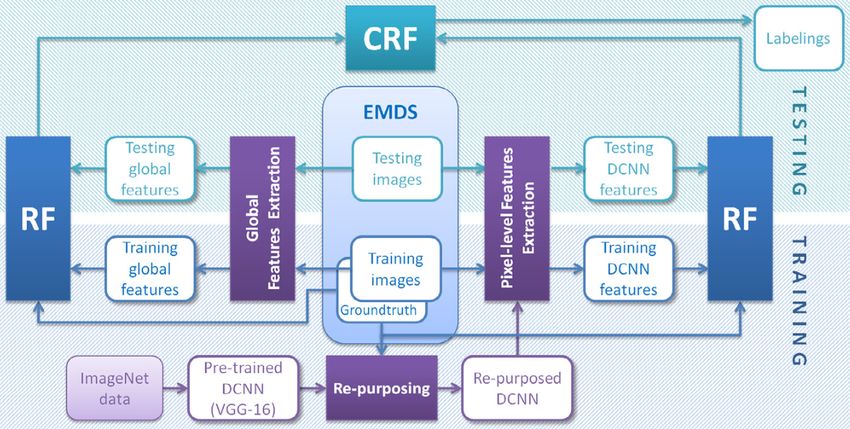
ecologists to analyse seawater samples has great significance. A system called
DiCANN is proposed for this purpose in [27]. This system consists of ANNs, an
Internet distributed database, and image analysis techniques. The image data
used in the experiment is derived from a Distributed Image Database (DIB)
on the Internet. As the system’s workflow shown in Fig. 10, the input image
data is pre-processed first, and then the features are extracted for training or
testing the classifiers. The classifiers contain back-propagation of error feed-
forward Perceptron (BPN), KNN, RBF, and QDA. The experimental results
are shown in Fig. 11. As the number of species increases, human performance
declines while the performance of BPN rises most obviously.
Fig. 10 The workflow of DiCANN in [27].
Fig. 11 The experimental results of DiCANNin [27].Title Suppressed Due to Excessive Length 17
In [5], four kinds of ANNs are applied to the classification task of Es-
cherichia coli, including MLP, RBF, General Regression Neural Network (GRNN),
and PNN. A total of 336 Escherichia coli instances are used in the experiment.
There are eight classes in the dataset. The experimental results show that PNN
is the most suitable model for Escherichia coli classification. Using this neural
network, the benchmark result using the ad hoc structured probability model
is improved to 82.97% correct classification rate.
Counting phytoplankton using a microscope is a time-consuming process.
Therefore, it is of great significance to develop an automatic counting system.
In [39], a phytoplankton identification and counting system based on com-
puter image analysis and pattern recognition is proposed. The system consists
of ANNs and simple rule-based procedures. The image data used in the ex-
periment is taken directly from water samples from Lough Neagh in northern
Northern Ireland. In the experimental process, the input image is pre-processed
and analysed first, then the 74 parameters describing size, shape, colour and
grey level distribution are extracted for the training of the network, and fi-
nally, the test data are used for testing. The experimental result shows that
the automatic system is close to the results obtained by manual.
Their own experience often influences human experts in the identification
of Cryptosporidium parvum and Giardia lamblia that can infect humans and
cause deadly gastroenteritis. ANNs are widely used in biomedical image iden-
tification in recent years. Therefore, the methods based on ANNs are proposed
to perform the identification task of these two protozoa in [152]. In the exper-
iments, the image data is first clipped to fit the input of the networks (40 by
40 and 95 by 95 pixels for Cryptosporidium parvum and Giardia lamblia, re-
spectively). The ANNs used for Cryptosporidium parvum and Giardia lamblia
have 1600 and 9025 input neurons. Both of them have five hidden and two
output neurons. In the experiments, there are 1586 and 2431 images for train-
ing Cryptosporidium oocyst ANN and Giardia cyst ANN, respectively. After
the training process, 100 images are used to select ANNs, which show the
best performance. Finally, Cryptosporidium oocyst ANN achieves 91.8% cor-
rect identification rate on 500 unseen images and Giardia cyst ANN achieves
99.6% correct identification rate on 282 unseen images.
The analysis of sedimentary organic matter can be used in geochronologi-
cal, biostratigraphical, paleoecological and paleoenvironmental analysis. How-
ever, the traditional microscope analysis is time-consuming and tedious. Au-
tomatic technology can improve effectiveness. Thus, in [149], a semi-automatic
system is presented to perform the classification task of sedimentary organic
matter. The image data used in the experiments are from Paleogene and
Holocene samples. The data can be divided into two orders. In the first order,
there are 3266 samples belong to three second order classes: 501 for second or-
der amorphous, 1475 for second order palynodebris, and 1290 for second order
palynomorphs. In the experiments, after image capture, the pre-processing is
applied to segment the foreground, and then 194 original features, including
morphological and textural features, are extracted. After that, the Exhaus-
tive CHi-square Automatic Interaction Detector classification tree algorithm18 Jinghua Zhang1,2 et al.
is used to determine the effective features for each ANN training. The ANNs
used here are back-propagation MLP. The Gamma test is used to prevent the
overtraining problem. The workflow of the system is shown in Fig. 12, the
classification contains two stages. In the first stage, the test image is classified
into the second order category, and then it is classified into a subcategory in
the second stage. The experimental results show that the system achieves an
average correct classification rate of 87%.
Fig. 12 The workflow of the system in [149].
The related image recognition methods are behindhand with the wide ap-
plication of optical imaging samplers in plankton ecology research. Most meth-
ods may need manual post-processing to correct their results. To optimize this
situation, a dual-classification method is proposed in [58]. As the workflow of
the dual-classification system shown in Fig. 13, four kinds of shape features, in-
cluding moment invariants, morphological measurements, Fourier descriptors,
and granulometry curves, are used to train a Learning Vector Quantization
Neural Network (LVQ-NN) in the first classification, and texture-based fea-
tures (co-occurrence matrix) are used to train the SVM to achieve the second
classification. Only when the results of the two classifiers are the same, can
the plankton be classified into one class, which effectively reduces the false
positive rate. The image data used in the experiments are collected from the
Great South Channel off Cape Cod, Massachusetts. It contains seven cate-
gories and a total of about 20000 images. The experimental results show that
compared with previous methods, the dual-classification system after correc-
tion can effectively achieve abundance estimation and reduce the error by 50%
to 100%.
It is a time-consuming and laborious task to analyse protozoa and meta-
zoa by observing through the microscope. It is of great significance to apply
digital image analysis technology in this analysis process. In [45], the authors
develop an image analysis program to perform the semi-automatic recogni-
tion of several protozoa and metazoa commonly used in sewage treatment.Title Suppressed Due to Excessive Length 19
Fig. 13 Schematic diagram of dual-classification system in [58].
The program uses around 40 morphological parameters to train Discriminant
Analysis and ANN to to identify and classify protozoan or metazoan images.
The experimental results show that this program can effectively distinguish
amoebas, sessile ciliates, crawling ciliates, large flagellates and free swimming
ciliates.
Protozoa and metazoa are good indicators in sludge treatment. Manual
analysis methods are time-consuming and have professional requirements for
operators. Therefore, the digital image analysis method has the potential capa-
bility in this task. In [44], a semi-automatic image analysis program is proposed
for protozoa and metazoa classification. The image data used in the experi-
ments are taken from 22 classes of protozoa and metazoa collected from aera-
tion tanks of WWTPs of Nancy (France) and Portugal treating domestic and
industrial effluents. In the program’s workflow, the image data is pre-processed
(filtering, segmentation, noise reduction, etc.) to generate the region of inter-
est. Then the morphological features are extracted for training the classifiers,
which includes discriminant analysis, neural network, and decision tree. The
neural network used here is a two-layer feed-forward neural network without a
hidden layer based on the BP algorithm. The experimental results show that
discriminant analysis and neural network are more suitable for this task, while
the decision tree is not.
It is tedious and time-consuming work to identify, count and measure in-
dividual cells manually. Image analysis methods are effective tools. In [157],20 Jinghua Zhang1,2 et al.
the authors present a novel method for bacterial image classification. In this
method, the image pre-processing is applied first, in which Iterative threshold
segmentation and mathematical morphology are proposed to realize bacte-
ria image edge detection, and then 20 original features are extracted. After
the feature extraction, eight effective features are selected by the Bayesian
model, and Principal Component Analysis (PCA) is used. These processed
features are used to train ANN, a three-layer feed-forward neural network, to
perform the classification. The data used in the experiments contains eight
bacteria classes, which are from National Microbe Culture Resource (NMCR)
database. There are 60 images used as a training set and 20 images for testing.
The accuracy of recognition rate in the experiments is 82.3%.
As an extension of work [157], different feature extraction and selection is
used in [154]. Six effective features are selected from 15 original features (four
morphological features, seven invariant moments, and four texture features) by
their variance contribution. Under the same experimental condition as [157],
the accuracy of recognition rate in [154] is 86.3%.
As an extension of work [149], a new version of the classification system is
proposed in [150]. Due to the ANNs used in the previous system show poor
performance on the first order and second order amorphous classification tasks,
RBF is used to replace back-propagation MLP in this work. The novel system
is shown in Fig. 14. The experimental results show that in the best case, the
correct recognition rate is improved by 4% to just over 91%.
Fig. 14 The workflow of the system in [150].
The determination of bacterial abundance, biovolume and morphology in
wastewater by manual analysis through a microscope is a time-consuming task.
Therefore, in [155, 29, 156], a bacteria image recognition system is proposed for
related research and application to solve the problem. In this system, adaptive
and enhanced edge detection is proposed for image pre-processing first. Then,
the original features, including contour Invariant moment and morphological
features, are extracted, and six effective features are selected from the originalTitle Suppressed Due to Excessive Length 21
features, and PCA is applied to reduce the features’ dimension. Finally, the
processed features are used to train an ANN to perform the classification
task. The ANN used here is a three-layer feed-forward neural network based
on an adaptive accelerated BP algorithm. The data used in the experiments
are from the CECC database. In the experiments, the adaptive accelerated BP
algorithm can effectively accelerate the training process by five times. Thirty
images from the CECC database are used to test the system’s performance,
and the result shows that the recognition rate is 85.5%.
Because the manual method to actived sludge screening is time-consuming
and laborious, it can be widely applied. In [4], a semi-automatic method is pro-
posed to perform the recognition task of stalked protozoa species in sewage.
In this method, the acquired images are segmented first, and then the fea-
tures, which contains geometrical, morphological and signature descriptors,
are extracted. Finally, the discriminant analysis and neural networks trained
by these features were used to identify stalked protozoa. The data used in the
experiments are collected from aeration tanks of WWTP in Nancy (France)
and Braga (Portugal). The main goal of this study is to find out the most ef-
fective feature class. The experimental results show that geometrical features
are the most important.
The development of a simple and reliable computer-aided microscopy method
to analyse complex microbial communities is a major challenge in microbial
ecology. In [52], a method for the classification of different cell growth phases
is introduced. In this method, the adaptive global thresholding is applied to
segment the cell images first, and then five geometric features, including cir-
cularity, compactness, eccentricity, tortuosity and length-width ratio, are ex-
tracted for training the classifiers. The classifiers contain 3σ, KNN, neural
network, and fuzzy classifiers. The neural network used in this study is RBF.
The dataset used here has three phases: normal or grownup or about-to-divide.
Each phase of the bacilli bacterial cell has 100 colour images. The experimental
results show that fuzzy classifier performs best, and the classification accuracy
of the three phases are 100%, 98% and 98%, respectively, while the neural net-
work is the second, and the classification accuracies are 100%, 96% and 95%,
respectively.
In [53, 55], an image analysis method used for cocci bacterial cell classifica-
tion is proposed. In this method, the image segmentation is performed by the
actived contour, and then five geometric features, which contain circularity,
compactness, eccentricity, tortuosity and length-width ratio, are extracted for
training and testing of the classifiers. There are three classifiers, 3σ, KNN, and
neural network classifiers, used in this study. The neural network is RBF. A
total of 350 image data is used in the experiment, with six categories: cocci,
diplococci, streptococci, tetrad, sarcinae, and staphylococci. The experimental
results show that the neural network achieves the best performance. According
to [53], the classification accuracy details of each class achieve by the neural
network are 100%, 99%, 98%, 99%, 98%, and 99%, respectively.
The traditional microorganism detection and identification method is labours
and time-consuming. In [71], a rapid and cost-effective method based on PNN,22 Jinghua Zhang1,2 et al.
whose structure is shown in Fig. 15, is applied to classify the microorganism
image classification task. The features, including various geometrical, opti-
cal, and textural parameters, are extracted from the pre-processed images to
train the network in this method. In the experiments, the dataset includes five
categories that are Bacillus thuringiensis, Escherichia coli K12, Lactobacil-
lus brevis, Listeria innocua, and Staphylococcus epidermis. The experimental
results show that the PNN based on nine kinds of features, which are 45◦
run length non-uniformity, width, shape factor, horizontal run length non-
uniformity, mean grey level intensity, ten percentile values of the grey level
histogram, 99 percentile values of the grey level histogram, sum entropy, and
entropy, can classify the microorganisms with 100% accuracy.
Fig. 15 The structure of probabilistic neural network in [71].
In environmental bacteria image acquisition, it is easy to generate low-
quality images, bringing troubles to the subsequent analysis. Therefore, a
computer-aid method based on ANN is introduced to perform the classification
task of different quality categories in [165]. The experimental data is private,
and it contains 25000 images with three categories: high quality, medium qual-
ity, and low quality. As the workflow is shown in Fig. 16, the input image is
divided into nine sub-images, and three features, including mean grey value
(MGV), background inhomogeneity (BGI), and cell density measure (CDM),
are extracted from each sub-image. Then the ANN is trained by the normal-
ization and sorting of the measured features. The network used in this study
consists of 27 input, 90 hidden, and three output neurons. The experimental
results show that the optimal ANN achieves a correct identification rate of
94%.Title Suppressed Due to Excessive Length 23
Fig. 16 The workflow of the system in [165].
The conventional manual method for detecting Mycobacterium tubercu-
losis is an ineffective but necessary part of diagnosing tuberculosis disease.
In [101], a method based on the image analysis technique and ANN is intro-
duced to detect the Mycobacterium tuberculosis in the tissue section. Fifteen
tissue slides are collected in the Department of Pathology, USM Hospital, Ke-
lantan, and each slide is captured to generate 30 to 50 images. A total of 607
objects, which contains 302 definite TB and 305 possible TB, are obtained.
In the experiments, the moving k-means clustering is applied to segment the24 Jinghua Zhang1,2 et al.
images, and geometrical features of Zernike moments are extracted. Then, the
Hybrid Multilayered Perceptron (HMLP) is used to test the performance of
different feature combinations in the detection task. Fig 17 provides an exam-
ple of HMLP with one hidden layer. The experimental results show that the
HMLP with the best feature combination can achieve an accuracy of 98.07%,
a sensitivity of 100%, and a specificity of 96.19%.
Fig. 17 An example of HMLP with one hidden layer in [101].
Similar to [52, 53], the same workflow is applied to classify three types of
spiral bacterial cells: are vibrio, spirillum, and spirochete in [54]. Same as [52],
3σ, KNN, neural network, and fuzzy classifiers are applied in this study. The
experimental results show 3σ, KNN (K = 5), neural network (RBF), and
fuzzy classifiers achieve 100% classification accuracy on the test data of three
categories. It proves that neural network can provide good classification ability.
Besides, in [56], the neuro fuzzy classifier is used to replace the fuzzy classifier
in [54], the results show that it shows the same performance as the fuzzy
classifier.
TB detection in tissue is more complex and challenging than detection
in sputum. In [100], a method based on the image processing technique and
ANN is introduced to detect and classify TB in tissue. The slides used in this
work are collected from the Pathology Department, Hospital Universiti Sains
Malaysia, Kelantan. The 1603 objects consist of three categories, which are TB,
overlapped TB, and non-TB, are collected from 150 tissue slide images. As the
workflow is shown in Fig. 18, the captured image is segmented first, and thenTitle Suppressed Due to Excessive Length 25
the features are extracted to train the network to perform the classification
task. The network is a single-layer feed-forward neural network trained by
Extreme Learning Machine. The experimental results show that the network
obtains a classification accuracy of 77.25%.
Fig. 18 The workflow of the detection method in [100].
As the extension of [100], a new method based on image processing tech-
nique and ANN is proposed in [99]. The data and workflow used in this study
are the same as [100]. The network used here is the HMLP network trained by
integrating both Modified Recursive Prediction Error algorithm and Extreme
Learning Machine. The results show that this network can achieve the highest
testing accuracy of 77.33% and average testing accuracy of 74.62% for 35 hid-
den nodes. Besides, in [103], similar work is presented. The data used in this
study contains 1600 objects consisting of TB, overlapped TB, and non-TB,
which are collected from 500 tissue slide images. A single hidden layer feed-
forward network trained by Online Sequential Extreme Learning Machine is
applied in this study. The experimental results show that the network trained
by geometrical features can achieve classification scores above 90.00% on three
categories.
It is essential but ineffective to analyze the sputum specimen by manual
methods. The digital image analysis method can effectively optimize this situ-
ation. In [121], a classification method based on ANN is introduced. A total of
100 images used in this study are the binary images directly taken from [41].
There are 75 and 25 images for training and testing, respectively. In the work-
flow of this method, geometry features, containing circularity, compactness,
eccentricity, and tortuosity, are extracted from the binary images for training
and testing the classifier. The network used here is BP based MLP. The ex-
perimental results show that the ANN can accurately classify the tuberculosis
bacteria or not with a mean square error of 0.000368.
Biomonitor is important for the researches related to the ecosystem. How-
ever, the manual identification method is ineffective. Therefore, [66] focus on
the automatic classification and retrieval of macroinvertebrate images. In thisYou can also read


