Temporal dynamics of tree xylem water isotopes: in situ monitoring and modeling
←
→
Page content transcription
If your browser does not render page correctly, please read the page content below
Biogeosciences, 18, 4603–4627, 2021
https://doi.org/10.5194/bg-18-4603-2021
© Author(s) 2021. This work is distributed under
the Creative Commons Attribution 4.0 License.

Temporal dynamics of tree xylem water isotopes:
in situ monitoring and modeling
Stefan Seeger and Markus Weiler
Hydrology, Faculty of Environment and Natural Resources, University of Freiburg, Freiburg im Breisgau, Germany

Correspondence: Stefan Seeger (stefan.seeger@hydrology.uni-freiburg.de)

Received: 12 February 2021 – Discussion started: 15 February 2021
Revised: 1 June 2021 – Accepted: 8 June 2021 – Published: 12 August 2021

Abstract. We developed a setup for a fully automated, high-       1     Introduction
frequency in situ monitoring system of the stable water iso-
tope deuterium and 18 O in soil water and tree xylem. The         Transpiration from terrestrial plants is a key component of
setup was tested for 12 weeks within an isotopic labeling         the global hydrological cycle, and its fraction of the to-
experiment during a large artificial sprinkling experiment in-    tal water balance might even increase under projected fu-
cluding three mature European beech (Fagus sylvatica) trees.      ture climatic conditions (Bernacchi and VanLoocke, 2015).
Our setup allowed for one measurement every 12–20 min,            Process-based ecohydrological models can be an important
enabling us to obtain about seven measurements per day for        tool to gain realistic estimates of the vegetation’s response to
each of our 15 in situ probes in the soil and tree xylem.         climatic changes. Such process-based models need detailed
While the labeling induced an abrupt step pulse in the soil       data on plant water uptake and transpiration. These processes
water isotopic signature, it took 7 to 10 d until the isotopic    can and have been studied intensively with the help of stable
signatures at the trees’ stem bases reached their peak label      water isotopes (White et al., 1985; Calder, 1991; Dawson and
concentrations and it took about 14 d until the isotopic sig-     Ehleringer, 1991; Busch et al., 1992; Ehleringer and Dawson,
natures at 8 m stem height leveled off around the same val-       1992; Zhang et al., 1999; Dawson et al., 2002).
ues. During the experiment, we observed the effects of sev-
eral rain events and dry periods on the xylem water isotopic      1.1    Isotope-tracer-enhanced observations of tree water
signatures, which fluctuated between the measured isotopic               dynamics
signatures observed in the upper and lower soil horizons. In
order to explain our observations, we combined an already         To observe the temporal dynamics of water within the soil–
existing root water uptake (RWU) model with a newly devel-        plant–atmosphere continuum (SPAC), isotopic labeling ex-
oped approach to simulate the propagation of isotopic signa-      periments offer a unique opportunity to create distinct pulses
tures from the root tips to the stem base and further up along    that can be traced from the soil, through the plant, to the
the stem. The key to a proper simulation of the observed          atmosphere. For small experimental plots, chamber-based
short-term dynamics of xylem water isotopes was account-          measurements can capture the isotopic composition of tran-
ing for sap flow velocities and the flow path length distribu-    spiration (δT ) following isotopically labeled irrigation pulses
tion within the root and stem xylem. Our modeling frame-          (e.g., Yepez et al., 2005; Volkmann et al., 2016a). Due to di-
work allowed us to identify parameter values that relate to       mensional limits set by the size of the required chamber, this
root depth, horizontal root distribution and wilting point. The   method is not applicable to adult trees.
insights gained from this study can help to improve the rep-         Larger-scale irrigation experiments were conducted in
resentation of stable water isotopes in trees within ecohydro-    green house experiments with around 15 m high tropical trees
logical models and the prediction of transit time distribution    (Evaristo et al., 2019) and in a central European forest with
and water age of transpiration fluxes.                            grown, 25 m high, specimens of Fagus sylvatica and Abies
                                                                  alba (Magh et al., 2020). Instead of chamber measurements
                                                                  of δT , they extracted water from tree crown branches to mon-

Published by Copernicus Publications on behalf of the European Geosciences Union.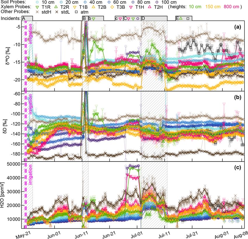
4604                                                  S. Seeger and M. Weiler: Temporal dynamics of xylem water isotopes

itor the isotopic composition of xylem water (δxyl ). For 7          The assumption that isotopic signatures of RWU (δRWU )
months, Evaristo et al. (2019) had a weekly δxyl sampling         are directly related to simultaneously sampled δxyl has been
scheme, while Magh et al. (2020) started with a sub-daily         challenged by studies of Knighton et al. (2020) and De Deur-
δxyl sampling scheme for 5 d and continued the following          waerder et al. (2020). Knighton et al. (2020) juxtaposed a
2 months with a sampling frequency of 4 to 6 d. Both ex-          “zero storage case” (δRWU = δxyl ) and two alternative cases
periments observed notable delays (days to weeks) between         (well mixed and piston flow) that included tree internal water
tracer application and detection within the sampled crown         storage. Model results for the cases with tree internal water
branches.                                                         storage compared better to observational data than the zero
   A more specific investigation of tree water dynamics can       storage case. Due to a limited temporal resolution of their ob-
be achieved by skipping soil and roots and directly inject-       served data, Knighton et al. (2020) were not able to conclude
ing small amounts of D2 O into the stem base (James et al.,       whether the piston flow or the well-mixed case was more ap-
2003; Meinzer et al., 2006; Schwendenmann et al., 2010;           propriate and hypothesized that the actual behavior of the
Gaines et al., 2016). Due to the high deuterium concentra-        system may lie between those two cases. De Deurwaerder
tions of the injected label, tracer breakthrough curves within    et al. (2020) proposed a model that comprised a soil-water-
the tree crown could be acquired by analyzing condensate          potential-driven RWU component and a stem water transport
from branch or foliar samples placed into zipper bags. Time       module that is based on an advection–diffusion model cou-
delays between tracer application and maximum tracer con-         pled to sap flow velocities. Based on their model, De Deur-
centrations within the tree crowns have mostly been reported      waerder et al. (2020) predicted that diel fluctuations of δRWU
to amount to a few days, but for a 50 m high specimen of          (caused by fluctuations in leaf water potential) should be
Tsuga heterophylla Meinzer et al. (2006) also reported a          transmitted from the stem base upwards, effectively causing
delay of about 30 d. A comparison of heat-tracing-derived         periodic patterns of δxyl along the stem height.
sap flux velocities with isotope-tracing-derived velocities re-
vealed that the latter may be 4 to 16 times higher (Meinzer       1.3   Measurement of soil and xylem water isotopes
et al., 2006; Gaines et al., 2016).
                                                                  Until recently, measurements of δxyl and isotopic composi-
1.2    Water uptake and tree isotope modeling                     tions of soil water (δsoil ) usually required the laborious ex-
                                                                  traction of the respective waters. Scholander pressure cham-
Rothfuss and Javaux (2017) have reviewed 159 studies com-         bers (Scholander et al., 1965) can be used to extract xylem
bining root water uptake (RWU) and isotopes. A total of 46 %      water from branches (Rennenberg et al., 1996; Magh et al.,
of those studies used isotopic data to infer a specific soil      2020). Another common xylem water extraction method is
layer or water pool as a source of RWU. Another 50 % of           cryogenic vacuum extraction (Dawson and Ehleringer, 1991;
those studies used two- or multi-source linear mixing mod-        Orlowski et al., 2013; Newberry et al., 2017), which is also
els of varying statistical sophistication. Only the remaining     commonly used for soil pore water extraction (Dalton, 1988).
4 % of the reviewed studies used physically based analytical      A detailed review on available soil pore water extraction
or numerical models. This means that the vast majority of         techniques was done by Orlowski et al. (2016). All of these
isotope-based RWU studies are based on graphic or statisti-       methods require destructive sampling of plant or soil mate-
cal methods, which allow a description of observations but        rial and subsequently careful sample storage and treatment.
abstain from offering physically based models, which could        The required effort per sample and the disturbance caused
be used to predict the reaction of RWU to changing environ-       by each sampling limit the total number of samples as well
mental conditions.                                                as the maximum sampling frequency. In fact, the very nature
   Lv (2014), Rabbel et al. (2018) and Brinkmann et al.           of destructive sampling renders repeated measurements from
(2018) have modeled RWU of trees with implementations of          the exact same spot impossible. Consequently, a time series
a Feddes-style RWU model described by Feddes et al. (1976)        generated with a destructive sampling method will inevitably
and Jarvis (1989) as implemented within the soil hydrologi-       also be affected by spatial variability.
cal model HYDRUS-1D (Šimůnek et al., 2008). Even though             With the advent of laser spectroscopy, the measurement of
the Feddes RWU model was originally developed to model            stable water isotopes does require the extraction of liquid wa-
water uptake of agricultural crops, the above-listed applica-     ter samples not any longer. Instead, the isotopic composition
tions demonstrated that Feddes RWU models are also suited         of the vapor contained in a gaseous sample can directly be
to simulate RWU of mature trees. Brinkmann et al. (2018)          analyzed in the lab and even in the field. Firstly, this leads to
used a Feddes RWU model, driven with soil water poten-            the development of equilibration-based lab methods which
tials and soil 18 O concentrations simulated with an isotope-     allow for indirect water isotope measurements from samples
enabled version of HYDRUS-1D (Stumpp et al., 2012), to            without the need for the extraction of liquid water from de-
compute δ 18 O signatures of RWU. These predictions com-          structive samples (Wassenaar et al., 2008; Garvelmann et al.,
pared well to fortnightly sampled δ 18 O values of branch         2012). Subsequently, different approaches for in situ sam-
xylem water.                                                      pling of stable water isotopes have been developed. For a

Biogeosciences, 18, 4603–4627, 2021                                                  https://doi.org/10.5194/bg-18-4603-2021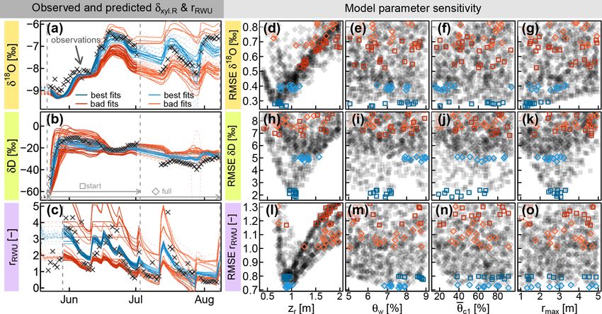
S. Seeger and M. Weiler: Temporal dynamics of xylem water isotopes 4605
thorough review of in situ water isotope sampling techniques 2 Methods
we would like to refer to Beyer et al. (2020).
Different approaches for in situ measurements of δsoil have 2.1 Theoretical basis
been proposed and tested by Soderberg et al. (2012); Roth-
fuss et al. (2013); Volkmann and Weiler (2014) and Gaj 2.1.1 Root water uptake model
et al. (2016). So far the method of Rothfuss et al. (2013) has
Following an RWU modeling approach established by Fed-
seen the most subsequent applications ranging from long-
des et al. (1976) and modified by Jarvis (1989), the contri-
term, continuous lab experiments (Rothfuss et al., 2015)
bution of different soil layers to total RWU can be described
to campaign-based field studies (Oerter and Bowen, 2017;
with the following equation:
Kübert et al., 2020). For in situ sampling of δxyl , Marshall
et al. (2020) developed the borehole equilibration method, N
X
which goes entirely without a specific probe and instead con- RWU = Si 1zi , (1)
nects tubing directly to a borehole through a stem. So far, this i=1
method only has been tested on cut trees that drew water up where i is the index of a specific soil layer, N is the total num-
through their stems under tension derived from transpiration ber of all soil layers and 1zi is the thickness of soil layer i.
and in a greenhouse experiment with small trees placed in According to Jarvis (1989), Si is the relative source strength
pots filled with water instead of soil. of soil layer i, which is defined by
The in situ probes developed by Volkmann and Weiler
(2014) are the only approach that has been proven to work Si = Ri αi , (2)
in soil (in six 2 d sampling periods; Volkmann et al., 2016a)
as well as within tree xylem (in two young Maple trees over where Ri is the proportion of total fine root length within
11 d; Volkmann et al., 2016b). While these probes have been layer i and αi is a stress index. Following a root distribu-
called SWIPs (soil water isotope probes) when used in the tion model introduced by Gerwitz and Page (1974) and Jarvis
soil and XWIPs (xylem water isotope probes) when used in (1989) defined Ri as
tree xylem, the actual probes in our study are identical in both
1zi zi
use cases. Therefore we propose an alternative third name: Ri = f exp −f . (3)
WIP (water isotope probe), which should encompass both zr zr
of the mentioned and all further use cases of this particular In this equation the tuning parameters zr and f are not inde-
probe design. pendent from each other – different combinations of the two
parameters lead to identical root distributions. For all further
1.3.1 Research objective considerations, we fixed the value of f to 3, which causes zr
to be the depth above which 95 % of all roots are located.
While stable water isotopes have been used for decades to
Jarvis (1989) computes the stress index α is as
study plant water uptake, a recent review on water ages by
Sprenger et al. (2019) notes that empirical evidence regard-
1−θ i
1−θ , θ c2 < θ i ≤ 1
ing the temporal dynamics of plant internal water remains
c2
limited. Studies by James et al. (2003), Meinzer et al. (2006), αi = 1, θ c1 ≤ θ i ≤ θ c2 (4)
Schwendenmann et al. (2010) and Gaines et al. (2016) have θi ,
0 ≤ θ i ≤ θ c1 ,
θc1
focused on tree xylem water transport between the stem base
and the crown, but their methodology neglected the possi- where θ c1 and θ c2 are critical values that define a trapezoidal
ble influence of the root system. Studies by Knighton et al. function that relates the normalized volumetric soil water
(2020) and De Deurwaerder et al. (2020) tried to model content θ to the water stress index α. θ is computed accord-
xylem water isotope transport with approaches of varying ing to
complexity but ultimately both studies were lacking compre-
hensive data sets with sufficient temporal resolution and cov- θi − θw
θi = , (5)
erage of soil and xylem water isotope data. θs − θw
The objective of this study was to make use of the unprece- where θi is a soil layer’s volumetric water content that lies
dented possibilities arising from the novel in situ measure- between wilting point θw and saturation θs .
ment approach based on the WIPs of Volkmann and Weiler Finally, the isotopic composition of RWU (δRWU ) can be
(2014) in order to investigate the temporal dynamics of tree computed by weighting the isotopic signatures of different
xylem water isotopes of a mature beech tree in a forest. soil layers (δi ) with their respective source strengths (Si ) and
Specifically, we wanted to examine the temporal relation be- thicknesses (1zi ):
tween the stable water isotopic signatures of RWU and stem
PN
xylem water. δi Si 1zi
δRWU = Pi=1 N
. (6)
i=1 Si 1zi
https://doi.org/10.5194/bg-18-4603-2021 Biogeosciences, 18, 4603–4627, 2021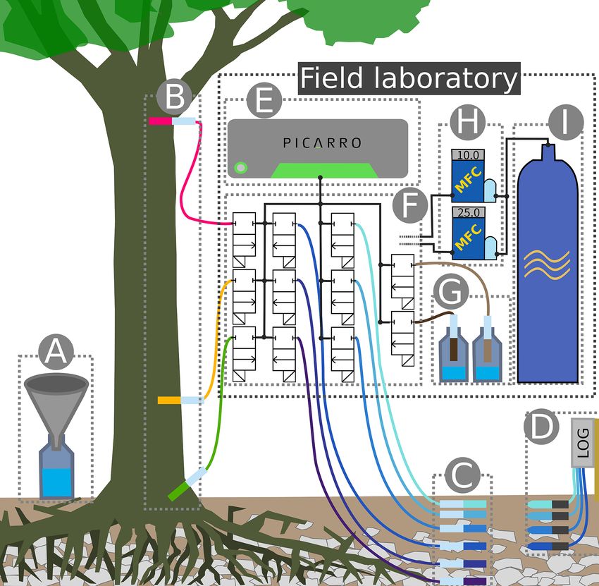
4606 S. Seeger and M. Weiler: Temporal dynamics of xylem water isotopes
2.1.2 Flow path length distribution
Root water uptake (RWU) happens at different depths and
different radial distances from the stem base. An isotopic
signature measured at the stem base will consequently rep-
resent a mixture of waters transported over various distances
(or flow path lengths) from the root tips to the stem. The flow
path length distribution (FPLD) of a tree root system is de-
termined by (1) a vertical component f (z), depending on the
soil depth z and (2) a radial component g(r), depending on
the radial distance from the stem center r.
The depth-dependent RWU probability function f (z) can
be defined by a mathematical function (like in Eq. 3) or by
empirical data of vertical fine root density distributions. The
radial RWU density function g(r) is, however, much less re-
ported and studied. In most cases, RWU is considered from a
one-dimensional perspective with regard to depth alone. For
our purposes we are also interested in the distribution of fine
roots regarding the radial distance from the stem. Due to a
lack of reported observational data, we propose the follow-
ing equation to describe possible relative root densities (in-
tegrated over all depths) along a radial transect between the Figure 1. Exemplary transformation of (d) a tracer concentration
center of the stem (r = 0) and the maximum radial extent of time series δ(t) to (a) a concentration function depending on the
the rooting system (r = rmax ): cumulative sap flow distance δ(s). A time series of (b) sap flow
velocities vsap (t) is needed for the construction of (c) the auxiliary
r
Bi ( rmax , λ, 1) function s(t).
gr (r) = 1 − , (7)
B(λ, 1)
with Bi being the incomplete beta function and B the com- theorem to compute the total distance to the stem base and
plete beta function. This equation is based on the cumula- aggregate hR (z, r) to the flow path length distribution hR (s):
tive density distribution of the beta distribution, and its shape
parameter λ determines how fast the root density is decreas-
X p
hR (s) = hR (z, r), for all z and r that fulfill z2 + r 2 = s.
ing with increasing horizontal distance from the stem (the
smaller the λ values, the faster the decrease; for λ = 1 the (10)
decrease is linear). In order to account for the effect of the
2.1.3 Signal transformation and convolution
projected area of a certain distance class, g(r) is computed
according to Inspired by a long line of tracer hydrological research (e.g.,
gr (r) rmax r Małoszewski and Zuber, 1982; Kirchner et al., 2000; Weiler
g(r) = R rmax x , (8) et al., 2003; McGuire and McDonnell, 2006) that uses con-
0 gr (x) rmax dx volution integrals to transfer precipitation tracer time series
to stream tracer time series via a transfer function, we adapt
where the denominator term normalizes the integral of g(r)
this approach to model the tracer dynamics within the tree
within 0 ≤ r ≤ rmax to unity.
xylem.
With the vertical component f (z) and the radial compo-
In order to neutralize the effects of sap flow velocity vari-
nent g(r) defined, both can be combined into a probability
ations, we transform our observed tracer time series δ(t) to
density function of RWU hR (z, r) in the following way:
“sap distance series” δ(s). This transformation is depicted in
hR (z, r) = Fig. 1 and it requires us to obtain a cumulative sap flow dis-
f (z1 )g(r1 ) f (z1 )g(r2 ) ... f (z1 )g(rj −1 ) f (z1 )g(rj )
tance s for each time step t with the following equation:
f (z2 )g(r1 ) f (z2 )g(r2 ) ... f (z2 )g(rj −1 ) f (z2 )g(rj )
... ... ... ... ... , n n n
f (zi−1 )g(r1 ) f (zi−1 )g(r2 ) ... f (zi−1 )g(rj −1 ) f (zi−1 )g(rj )
X X X
f (zi )g(r1 ) f (zi )g(r2 ) ... f (zi )g(rj −1 ) f (zi )g(rj ) s= 1si = 1ti (1si /1ti ) = 1ti vi , (11)
(9) i=1 i=1 i=1
where z1 , z2 , . . .zi−1 , zi and r1 , r2 , . . .rj −1 , rj denote suffi- where 1si is the distance traveled by the sap during ti , and
ciently finely spaced values of z and r within the respective 1vi is the mean sap flow velocity of ti , which has a duration
domains of f (z) and g(r). Now we can use the Pythagorean of 1ti . With an established transformation between time t
Biogeosciences, 18, 4603–4627, 2021 https://doi.org/10.5194/bg-18-4603-2021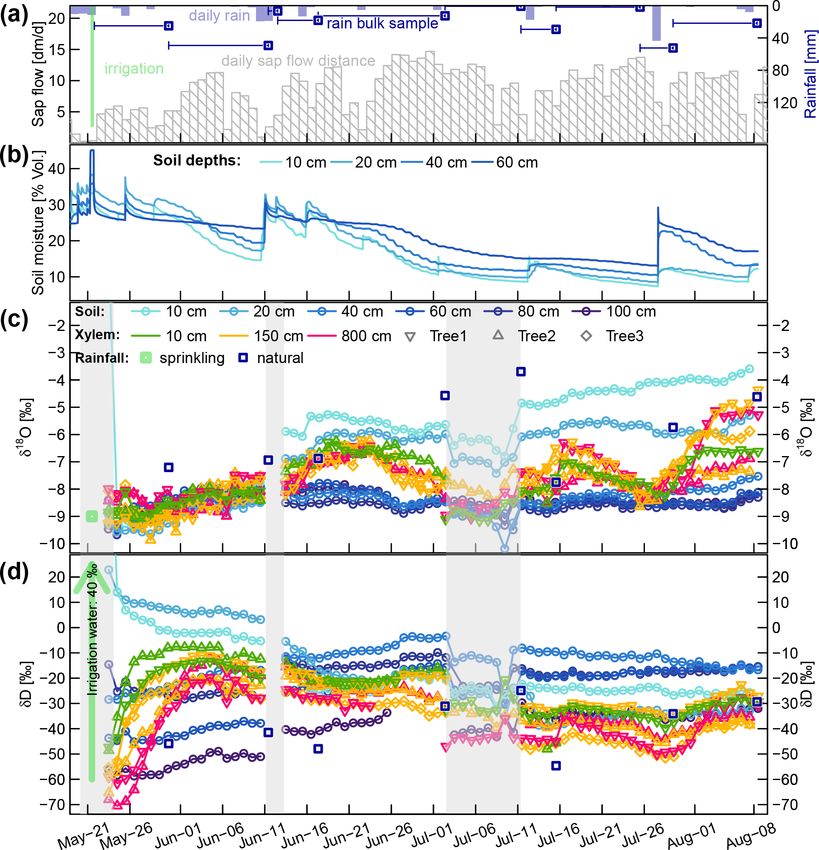
S. Seeger and M. Weiler: Temporal dynamics of xylem water isotopes                                                             4607

and sap flow distance s, we can transform observed tracer
time series δ(t) to tracer “sap flow distance” series δ(s).
   After the transformation of δ(t) to δ(s), we can predict
the isotopic signature at the stem base, δxyl.R , by convolving
δRWU with the FPLD between the stem base and all root tips
(e.g., hR from Sect. 2.1.2):

            Z∞
δxyl.R (s) = hR (s 0 )δRWU (s − s 0 )ds 0 .               (12)
             0

   Similarly, we can relate δxyl.R to δxyl.H (an isotopic stem
xylem signature at a certain height above the stem base) by
convolution with an appropriate transfer function that man-
ages to represent the respective FPLD.
   Eventually the methodology described in the previous sec-
tions can be combined as follows:

  – transform input tracer time series to input tracer sap dis-
    tance series,

  – convolve input tracer sap distance series with an appro-      Figure 2. Sketch of the experimental setup: (A) throughfall sam-
    priate transfer function (representing a static FPLD),        pler; (B) WIPs at 10, 150 and 800 cm stem height; (C) WIPs in 10,
                                                                  20, 40, 60, 80 and 100 cm soil depth; (D) volumetric soil moisture
                                                                  sensors in 10, 20, 40 and 60 cm depth; (E) CRDS for stable wa-
  – transform output tracer sap distance series back into an
                                                                  ter isotope measurements; (F) valve system to sequentially connect
    output tracer time series.
                                                                  each probe to the CRDS and the two mass flow controllers; (G) stan-
                                                                  dard probes in headspace of liquid water standards; (H) mass flow
2.2     Field experiment                                          controllers; (I) dry air for sample dilution and through-flow.
2.2.1    Study site and instrumentation

The experiment described in this study took place at a re-            At depths of 10, 20, 40, 60, 80 and 100 cm we installed
search site located on a 25◦ steep hillslope of the Swabian       one profile of WIP into the soil (Fig. 2F). Additionally we
Jura in southwestern Germany (47.98◦ N, 8.75◦ E, close to         installed WIPs into the xylem of two beech trees (T1 and
the city of Tuttlingen). The soil type is a Rendzic Leptosol      T2) at 10, 150 and 800 cm height (Fig. 2B), as well as
developed on glacial slope debris of Jurassic limestone. Soil     into the xylem of another beech tree (T3) at 150 cm height.
texture in the upper 70 cm ranges from silty clay to silty loam   The different installation heights are reflected by the probe
with a fraction of up to 43 % of rocks. Larger rock fragments     IDs (e.g., T1R, T1B and T1H), where R stands for “root”
can be found as shallow as 20 cm below the soil surface and       (10 cm), B for “breast height” (150 cm) and H for “high”
become very abundant below 50 cm. Our 200 m2 experimen-           (800 cm). Depending on the locations of the probes and the
tal plot was situated within a stand of 90–100-year-old Euro-     trees, the tubing lengths between the probes and the CRDS
pean beech (Fagus sylvatica) with diameters at breast height      varied between 5 m (T2R and T2B) and 20 m (T1H). Addi-
ranging from 45 to 90 cm and contained a total of four beech      tionally, we put two probes into the head space of two sealed
trees, of which three have been instrumented.                     1 L containers made of high-density polyethylene (HDPE),
   A sketch of the experimental setup is shown in Fig. 2,         filled with 250 mL of water with known isotopic composi-
which omits the repeated instances of the principal compo-        tion (Fig. 2E). These two probes acted as our light (δ 18 O =
nents and sensors. Precipitation (throughfall) samples were       −11.61 ‰, δD = −82.4 ‰) and heavy (δ 18 O = −0.93 ‰,
taken as often as possible from four rain gauges (Fig. 2A)        δD = 6.63 ‰) reference standards and were placed directly
distributed on and around the study plot. One of those            next to the CRDS in our field lab.
gauges was combined with a tipping bucket (0.2 mm reso-               In order to install the WIPs with a diameter of 10 mm into
lution, Davis Instruments, Hayward, USA) in order to regis-       the tree xylem, we drilled a hole with a 10 mm wood drill,
ter hourly precipitation amounts. A total of four depth pro-      a strip of tape marking a hole depth of slightly more than
files of volumetric soil moisture sensors (SMT100, Truebner       the length of the 5 cm porous head. Care was taken not to
GmbH, Neustadt, Germany) were installed in depths of 10,          overheat the drill in order to avoid singed xylem wood in the
20, 40 and 60 cm (Fig. 2G) with different radial distances to     hole. Afterwards, a 10.2 mm metal drill was used to slightly
the trees.                                                        widen the hole and clear out wood chip residue. Then the

https://doi.org/10.5194/bg-18-4603-2021                                                   Biogeosciences, 18, 4603–4627, 2021
4608                                                   S. Seeger and M. Weiler: Temporal dynamics of xylem water isotopes

probe was firmly pushed into the hole just deep enough to          filled into aluminum-coated coffee bags (WEBAbag CB400-
place the porous head behind the phloem. In a final step, sili-    420siZ, Weber Packaging GmbH, Güglingen, Germany).
cone was applied around the probe to seal the hole. While the          Following the equilibration bag method after Wassenaar
silicone is curing, organic fumes may interfere with the mea-      et al. (2008) and Garvelmann et al. (2012), the sample bags
surements of the CRDS. Therefore it is advisable to install        were filled with dehumidified air in the lab and permanently
the probes several days before the scheduled start of the mea-     sealed with sealing tongs (Weber Packaging GmbH). After
surements. In addition, we placed heat-pulse-based sap flow        24 h of equilibrium at constant temperature, the sample bags
sensors (East 30 Sensors, Pullman, USA) in the vicinity of         were punctured by a hollow needle connected to the inlet port
each WIP. Measurements of the tipping bucket, soil moisture        of a cavity ring-down spectrometer (CRDS) stable water iso-
sensors and sap flow sensors were logged in 10 min intervals       tope analyzer (L2120-I, Picarro, Santa Clara, USA). After
with a CR1000 data logger (Campbell Scientific, USA).              5 to 10 min, the isotope analyzer readings reached plateaus
                                                                   of constant values. Before and after the measurements of
2.2.2   Tracer experiment                                          the soil bags, we also measured three standard bags filled
                                                                   with liquid water of known isotopic composition, which were
The stable water isotope concentrations for 18 O and deu-          treated identically to the bags containing soil samples.
terium in this paper are noted in the δ-notation relative to           The WIPs used in this study were built at the Chair of Hy-
Vienna standard mean ocean water (VSMOW):                          drology of the University of Freiburg, Germany, following
                                                                 the “diffusion-dilution sampling” (DDS) design described
                 Rsample                                           by Volkmann and Weiler (2014). Figure 3 shows a sketch
δsample =                − 1 × 1000 ‰,                     (13)
                RVSMOW                                             of a WIP installed in the soil. Key elements of a WIP are
                                                                   the mixing chamber (B) made of PVDF and a screw-on
where Rsample and RVSMOW are the D/H or 18 O/16 O ratios           membrane head (C). This membrane head (manufactured
of the sample and VSMOW, respectively.                             by Porex Technologies, Aachen, Germany) mainly consists
   Since no direct water source was available to irrigate the      of a 50 mm long hydrophobic but vapor-permeable microp-
plot with a defined amount of 150 mm, 60 m3 of groundwater         orous cylinder made of PE with a pore size of 10 µm. From
was trucked to the site and run through an industrial deion-       within the mixing chamber, the sample line (D) connects to
izer (VE-300 (6 × 50 L), AFT GmbH & Co.KG) to reduce               the CRDS water isotope analyzer, which has a constant in-
the mineral content to low levels typically found in natural       take rate of about 35 mL min−1 . Air and vapor from within
rainfall. In our case the sprinkling water had an electrical       the probe head reach the mixing chamber through a small
conductivity of around 20 µS cm−1 and an isotopic compo-           connection hole and are sucked into the sampling line. The
sition of δ 18 O = −9 ‰ and δD = −63 ‰. By mixing 1 kg             dilution line (E) is used to deliver dry air directly into the
of D2 O with the 60 000 L of water within a collapsible pil-       mixing chamber, which allows for a controlled dilution of
low tank (custom made by FaltSilo GmbH, Bad Bramstedt,             the sampled air–vapor mixture, while the water outside of
Germany), which was placed 100 m upslope of the experi-            the probe and the air inside the probe head can still exchange
mental plot, we obtained deuterium-enriched irrigation wa-         under equilibrium conditions. The through-flow line (F) can
ter (δ 18 O = −9 ‰, δD = 40 ‰). On 21 May 2019, we used            deliver additional dry air into the system and helps to prevent
an array of six sprinklers (Xcel-Wobbler by Senninger, Cler-       underpressure as a result of dilution rates that are smaller
mont, USA) driven by the height difference between pil-            than the constant sampling rate. Tests have shown that the
low tank and irrigation site, to distribute our prepared D2 O–     gas exchange through the membrane head is so fast that it is
groundwater mixture onto the experimental plot. The amount         not possible to dilute the sampled air through the through-
of irrigation water actually reaching the core plot area of 10     flow line. All three lines of tubing utilized to deliver dry air
by 20 m was equivalent to 150 mm rainfall within 8 h. After        into the probe or sample vapor from the probe are made of
this artificial event, we continued to monitor the plot under      fluorinated ethylene propylene (FEP) and have an external
natural conditions for another 12 weeks.                           diameter of 1.59 mm (= 1/1600 ) and an internal diameter of
                                                                   0.75 mm.
2.2.3   Stable water isotope measurement system                        Deviating from the original applications of WIPs (Volk-
                                                                   mann and Weiler, 2014; Volkmann et al., 2016a, b), we
On 2 d prior to the irrigation, as well as 1 d after the irriga-   switched from using N2 as dilution and through-flow gas to
tion, we took a total of five destructive soil core samples. We    compressed dry air. As Gralher et al. (2018) have shown,
used an electric breaker (HM1812, Makita Werkzeug GmbH,            intrusion of ambient air has a considerably larger influence
Germany) to drive a core probe (60 × 1000 mm, Geotechnik           on measurements relying on N2 , compared to measurements
Dunkel GmbH & Co. KG, Hergolding, Germany) into the                that use dry air as dilution and flush medium. Furthermore,
soil until we hit larger rocks. The soil cores were extracted      transporting compressed dry air in a vehicle has fewer re-
and split into 10 cm segments, yielding 120 to 300 g of fine       strictions than transporting compressed N2 . A pressure reg-
soil and skeleton material per depth increment, which were         ulator reduced the pressure at the outlet of the compressed

Biogeosciences, 18, 4603–4627, 2021                                                   https://doi.org/10.5194/bg-18-4603-2021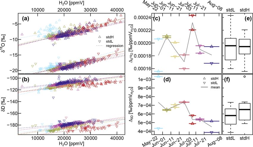
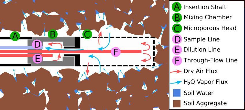
S. Seeger and M. Weiler: Temporal dynamics of xylem water isotopes                                                                 4609

Figure 3. Sketch of a WIP installed in soil. Water vapor from the surrounding medium (in this case soil) diffuses through the microporous
membrane into the probe head (C). Before being sucked into the sample line (D), the sample gas is diluted within the mixing chamber (B).

dry air bottle down to 1.5 bar. The dry air stream was split           Table 1. Threshold values for standard deviation s and trend index
between two mass flow controllers (GFC17, 0–50 mL min−1                IT used for automated detection of stable measurement values.
and MFC 35828, 0–200 mL min−1 , both manufactured by
Analyt-MTC GmbH, Müllheim, Germany).                                                                     Threshold values
   Over custom manufactured valve manifolds (Horst Fischer                            Parameter (unit)     s           IT
GmbH, Gundelfingen, Germany), equipped with two-way                                   H2 O (ppmV)        200          150
electric valves (EC-2M-12, Clippard, Cincinnati, USA), each                           δ 18 O (‰)          0.2          0.1
of the probes was connected to the two mass flow controllers                          δD (‰)                1          0.5
and the sample inlet of the field-deployed CRDS stable wa-
ter isotope analyzer (L1102-i, Picarro, Santa Clara, USA).
Connections between the probes, valve manifolds, mass flow             codes of the control software) can be found in the following
controllers and isotope analyzer were made with 1/16 in.               online repository: https://github.com/stseeger/IsWISaS (last
FEP tubing (Techlab GmbH, Braunschweig, Germany) and                   access: 8 July 2021).
flangeless fittings (XP-220, IDEX, Lake Forest, USA). Con-                In order to obtain a measurement value for a certain probe,
nections between the dry air supply and the mass flow con-             we activated the three respective valves of that probe (sam-
trollers were made with stainless-steel fittings (Swagelok,            ple, dilution and through-flow line). The time of activation
Solon, USA). We set up our field-deployed CRDS and its                 was saved to an automatically generated log file. At the
peripherals within a watertight container and supplied it with         same time, we initiated a flush phase by setting the dilu-
electricity from a nearby power line.                                  tion rate to the same as the CRDS’ sample intake rate (in our
   Based on the Arduino microcontroller platform                       case 35 mL min−1 ) and setting the flow rate in the through-
(Badamasi, 2014), we designed and built a custom cir-                  flow line to zero. The duration of the flush phase was cho-
cuit board that is able to switch electromagnetic valves               sen depending on the overall tubing length of the probe –
and to provide two independent analogue voltages. Those                from 3 min for probes with short tubing up to 10 min for
voltage signals were used to control the through-flow of               probes with 20 m long tubing. After the flush phase, we
two mass flow controllers. A custom-made Python-based                  started the measurement phase by reducing the dilution flow
software GUI that is able to interface the Arduino-based               rate to 10 mL min−1 and increasing the through-flow rate to
circuit board and interpret the CRDS’ log files in near-real           25 mL min−1 – dilution and through-flow yet again adding
time enabled us to automate the measurement process to a               up to the constant sample flow rate of the CRDS. The mea-
large extent and to quickly adapt flow rates and times for             surement phase either ended after a fixed amount of time (in
flushing and measuring as well as the order of the probe               our case 20 min) or earlier, in case the measured raw values
sequence. We attached a USB modem (E531, Huawei                        of the CRDS approached a stable plateau. Plateau detection
Technologies, Shenzhen, China) to the isotope analyzer to              was automated by checking standard deviations s and a trend
regularly transmit summarized measurement results (less                index IT of the last 2 min of CRDS raw data for H2 O (sample
than 20 kB h−1 ) to an FTP server. With this setup, we                 moisture content), δ 18 O and δD against the thresholds listed
could remotely monitor but not interfere with the ongoing              in Table 1. The standard deviation s was computed as
measurements. Further details on this automation system
(circuit board designs, assembly instructions and source

https://doi.org/10.5194/bg-18-4603-2021                                                        Biogeosciences, 18, 4603–4627, 2021
4610                                                      S. Seeger and M. Weiler: Temporal dynamics of xylem water isotopes

                                                                       moisture (averaged across the four available depth profiles)
  v                                                                    – more specifically the daily decline of soil moisture during
               N
  u
  u       1 X                                                          dry days – as an indicator of RWU. To compare the soil mois-
s=t               (xi − x)2 ,                                  (14)    ture measurements with the RWU model, we derived a water
        N − 1 i=1
                                                                       uptake ratio rRWU in two ways:
where N is the number of raw instrument readings within                           1θ u  Su
the last 2 min, x1 , x2 , . . ., xN are all of the respective values   rRWU =          = ,                                         (18)
                                                                                  1θl   Sl
and x is the mean of all these values. With the value of N/2
rounded to a whole number, the trend index IT was computed             where the first ratio defines the measured daily decline of soil
as                                                                     moisture in the upper soil layer 1θ u (average of 10 and 20 cm
       PN/2         PN                                                 depth) and 1θl the equivalent for the lower soil layer (aver-
          i=1 xi       i=N/2+1 xi                                      age 40 and 60 cm depth). The second ratio defines the relative
IT =             −                     .                        (15)
         N/2          N − N/2                                          modeled uptake strengths of Eq. (2) (with S u as the average
                                                                       of S i for the depths of 10 and 20 cm and S l as the average of
  After each probe measurement, the system automatically
                                                                       S i for the depths of 40 and 60 cm). The soil-moisture-based
proceeded to flush and measure the next probe within the
                                                                       computation of rRWU is limited to days where the soil water
specified probe sequence, which was automatically restarted
                                                                       content throughout the depth profile is below field capacity.
upon its completion.
                                                                          In order to analyze the WIP measurements, we used the
2.3    Data processing                                                 recorded valve switching times to aggregate the raw CRDS
                                                                       log file data by computing average values for the last 2 min
From the raw sensor data, we computed the sap flow velocity            of each period. The parameters of interest were sample water
vsap in m s−1 according to Campbell et al. (1991):                     vapor content, δ 18 O and δD. In the next step we corrected
                                                                     for the influence of temperature on the fractionation factors
             2k            1T u                                        during vapor equilibration at the probe head. Instead of di-
vsap =                ln          ,                    (16)
        Cw (ru + rd )      1T d                                        rect temperature measurements, we relied on the assump-
                                                                       tion that the temperature at the place of equilibration (i.e.,
where k is the thermal conductivity of sapwood set to                  around the probe head) is reflected by the water vapor con-
0.5 W m−1 K−1 (Hassler et al., 2018), Cw is the specific               tent of the obtained sample gas – given that the sample rate
heat capacity of water at 4.184 × 10⁶ m3 K−1 , ru and rd               and the dilution rate are held constant. By computing lin-
(both = 6 mm) are the distances of the central heater needle           ear regressions between measured vapor isotope values (δm )
to the up- and downstream thermistor needles, and 1T u and             for our two standards and the sample gas moisture contents
1T d refer to the temperature changes induced by the heating           (Cm ), we derived the slopes needed to correct all vapor iso-
pulse at the up- and downstream needles, respectively.                 tope measurements to one reference moisture content value
    Our measured sap flow time series was limited from May             (Cr = 18 000 ppmV) according to the following equation:
2019 to 8 August 2019. In order to extend it to the whole
year, we assumed no sap flow during the time where our de-             δv = δm − 1Cδ (Cr − Cm ),                                   (19)
ciduous trees did not have any foliage (before May and after
October). During those periods, we set vsap to 0 m s−1 . For           where δv is the corrected isotope value and 1Cδ is the slope
the remaining period between 8 August and 31 October, we               obtained by the linear regression between Cm and δm values
fitted the two parameters a and b of the following equation:           of the standards.
                                                                          To infer the isotopic signature of the liquid water that equi-
vsap = VPD × a/(VPD + b),                                      (17)    libriated with the sampled vapor, we used the relationship
                                                                       between the known liquid phase values of our two standards
where VPD is the vapor pressure deficit (derived from mete-            and the respective observed vapor values:
orological data of the nearby meteorological site Klippeneck
of the German Weather service DWD). In order to account                         δv.x − δv.L
                                                                       δl.x =               + δl.L ,                               (20)
for decreasing vsap due to leaf senescence, we multiplied the                      1LH
estimates obtained by Eq. (17) with a linearly decreasing re-
                                                                       where δl.x is the normalized liquid phase isotopic value of
duction factor between the middle of September and end of
                                                                       measurement x, δv.x is the moisture-corrected vapor value of
October. Urban et al. (2015) reported a comparable autumnal
                                                                       measurement x, δv.L is the moisture corrected vapor value of
reduction of sap flow in relation to potential evaporation for
                                                                       the light standard, δl.L , is the liquid phase isotopic value of
central European beech trees.
                                                                       the light standard and 1LH is the slope obtained by
   As an additional means to investigate RWU independently
of isotope measurements, we followed Guderle and Hilde-                          δv.L − δv.H
brandt (2015) and used measurements of volumetric soil                 1LH =                 ,                                     (21)
                                                                                 δl.L − δl.H

Biogeosciences, 18, 4603–4627, 2021                                                          https://doi.org/10.5194/bg-18-4603-2021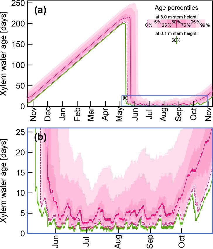
S. Seeger and M. Weiler: Temporal dynamics of xylem water isotopes                                                                  4611

with δv.H as the moisture corrected vapor value of the heavy        Table 2. The different parameters used for RWU modeling and the
standard and finally δl.L and δl.H as the known liquid water        transfer functions used to transform δRWU into δR (hR , hF1 ) and δR
isotope values of the light and heavy standards, respectively.      into δH (hF2 ). Meanings of the parameters are listed in Table A1.
   Under stable environmental conditions, δv.L and δv.H
should not change at all, but in a field experiment more fre-              Parameter    Model        Optimization     Final value
quent measurements of these standards are highly recom-                                                     range
mended. We treated both standards as regular parts of our                  θw           RWU             5 %–10 %             8%
measurement sequence, yielding one measurement of each                     θs           RWU                  45 %           45 %
standard every 3 to 4 h. For the normalization procedure we                θc1          RWU            10 %–90 %            40 %
interpolated between those actually measured standard val-                 θc2          RWU                 100 %         100 %
ues in order to estimate the standard values for each mea-                 zr           RWU, hR           0.4–2 m          0.9 m
surement.                                                                  rmax         hR                  1–5 m            3m
                                                                           λ            hR                 0.1–20             20
2.3.1   Modeling RWU, FPLDs and xylem water age                            α1           hF1                  1–30            3.4
                                                                           β1           hF1                  0.5–3          1.43
To obtain the necessary input data for RWU modeling, we                    γ1           hF1                    0m            0m
interpolated our observations of volumetric soil moisture and              α2           hF2                  0.1–3          0.62
soil isotopic signatures over time and space to generate a con-            β2           hF2                  0.5–3           1.3
                                                                           γ2           hF2                 0–5 m         1.64 m
tinuous time series in time and space. Lacking any observa-
tions below 60 cm for volumetric soil moisture and 1 m for
soil water isotopes, we assumed constant boundary condi-
tions (θ = 25 %, δ 18 O = −10.5 ‰ and δD = −73 ‰) at the            to a fixed value of 100, so that its first parameter α acts as
lower profile border in 2 m depth.                                  shape parameter while the additional parameters β and γ act
    Subsequently, we used the Jarvis RWU model (see                 as scale and lag parameters, respectively.
Sect. 2.1.1) to compute RWU isotopic signatures. Then we               Apart from simply predicting the transformation of δRWU
applied the convolution approach described in Sect. 2.1.2           during its transmission through a tree’s xylem, the fitted
in order to transfer the RWU isotopic signatures to the re-         FPLDs were also used to infer time variable xylem water age
spective stem base xylem isotopic signatures, which could           distributions. This was achieved by applying the approach
be compared to our in situ xylem water measurements at the          described in Sect. 2.1.3 in combination with a series of vir-
stem base. Model performance was evaluated by computing             tual tracers, one for each time step with a concentration of 1
the root-mean-square error (RMSE) between model predic-             during the respective time step and 0 during all other time
tions and observations for deuterium and 18 O at the stem base      steps. The resulting tracer concentration time series were
as well as for the water uptake index rU (see Sect. 2.3). With      used to infer xylem water ages similar to Sprenger et al.
yˆi as the ith of a total of n observations and yi as the respec-   (2016) (ages of percolation water below the root zone) and
tive simulated value, the RMSE was computed according to            Brinkmann et al. (2018) (ages of RWU water). In contrast to
            s                                                       the two mentioned studies, the water ages in this study refer
              Pn                2
                 i=1 (yˆi − yi )
                                                                    to the time of tree water uptake, instead of the time of input
RMSE =                            .                          (22)   as precipitation into the system.
                       n
   Next, we evaluated the model for 500 random parameter
sets within the value ranges given in Table 2. The soil re-         3     Results
lated model parameters were assumed to be identical over
the whole profile depth. Based on the observed soil moisture        3.1    Soil moisture and sap flow
time series, we set the volumetric soil moisture at saturation
θs to a fixed value of 45 %. Since soil moisture levels near sat-   The temporal dynamics of daily sap flow velocities and soil
uration only occurred for a short time during the irrigation,       moisture (averaged across the two profiles on the irrigated
we set the model parameter θ c2 to a value of 100 %.                plot) are depicted in Fig. 4a and b. Averaged for each month,
   Eventually, to relate modeled RWU to our observed xylem          the mean daily sap flow velocities varied between 42, 88, 94
isotopic signatures at stem heights of 0.1 and 8 m, we opti-        and 85 cm d−1 for May (starting at 21 May), June, July and
mized FPLDs that can be described by the following para-            August (ending at 8 August), respectively.
metric distribution:                                                   The sprinkling experiment started on 22 May during a
                                                                  wet period with soil moisture around field capacity (ca.
                       s −γ
hF (s; α, β, γ ) = F         ; α, 100 ,                     (23)    30 Vol. %). From 1 to 10 June, the first dry period oc-
                         β                                          curred, with soil moisture in the topsoil decreasing towards
with F being the probability density function of the Fisher–        15 Vol. %. Several rain events between 10 and 15 June rewet-
Snedecor distribution. The second parameter of F was set            ted the soil, but afterwards the soil moisture in all depths

https://doi.org/10.5194/bg-18-4603-2021                                                      Biogeosciences, 18, 4603–4627, 2021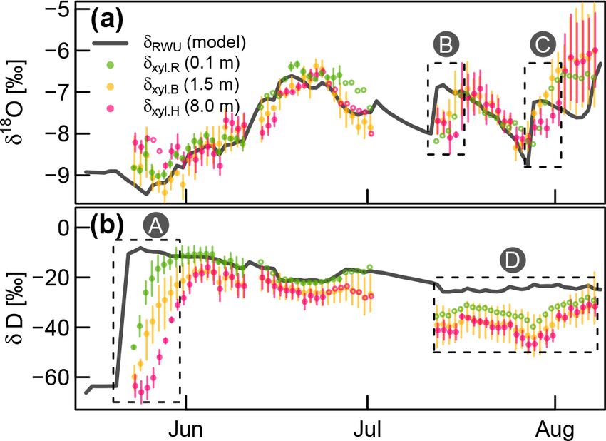
4612                                                      S. Seeger and M. Weiler: Temporal dynamics of xylem water isotopes

Figure 4. (a) Daily rainfall and cumulative sap flow distances. Dark blue squares represent the mean rainfall amounts collected with the four
bulk samplers (dark blue lines indicating the periods over which the bulk samples were collected). (b) Volumetric soil moisture at four soil
depths. (c and d) Corrected time series of δsoil and δxyl in liquid water. The blue squares represent the mean isotopic signatures of the four
bulk samplers. The translucent grey areas in (c and d) mark time periods with missing or unreliable isotope data.

declined considerably. One rainfall event with 29 mm on                  3.2    Stable water isotopes
12 July caused a brief rewetting of the topsoil, and a heavy
convective event with 52 mm on 27 July bypassed the up-
per two soil moisture probes and caused a strong increase by             In each measurement sequence 15 probes (two standards, six
around 10 Vol. % at 40 and 60 cm depth.                                  SWIPs and seven XWIPs) were measured within 3 to 5 h,
   The fitted Eq. (17) established a solid relationship (R 2             resulting in one measurement every 12 to 20 min. The raw
of 0.85) between vsap and VPD (see Fig. A4a). Since there                aggregated measurements and the correction procedure are
are no systematic discrepancies between measured and VPD-                described in Appendices A1 and A2. Some short-term fluc-
derived vsap values (see Fig. A4a), we have high confidence              tuations in the high-frequency data caused by diel air tem-
in assuming that the observed periods of reduced vsap during             perature fluctuations could be observed that could not com-
June and July (see Fig. 4a) can be attributed to temporarily             pletely be removed by the postprocessing procedures. Due to
lowered VPD instead of soil water deficits.                              the large number of data points in the full data set and our
                                                                         interest in the overall temporal dynamics, we limited our fur-
                                                                         ther analysis to daily median values of the full data set, set-

Biogeosciences, 18, 4603–4627, 2021                                                           https://doi.org/10.5194/bg-18-4603-2021
S. Seeger and M. Weiler: Temporal dynamics of xylem water isotopes 4613
ting aside the development of a more robust diel calibration 3.3 Optimization of the RWU model
procedure for future studies.
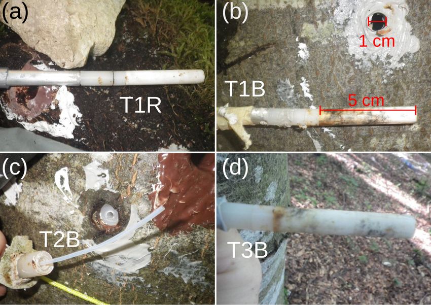
Three of the xylem probes (T1B, T2B and T3B) exhibited The temporally and spatially continuous soil moisture and
a negative δ 18 O bias, which was corrected as described in soil water isotope data needed for the optimization of the
Appendix A2.2. A comparison of the probe heads right after RWU model were obtained by interpolation of soil sensor
removal from the stem (12 weeks after installation) revealed data, soil core measurements and SWIP measurements (see
that the membrane heads of two δ 18 O-biased probes were Fig. A5).
covered by biofilms while an unbiased probe did not show Subsequently, the optimization was carried out as de-
such a biofilm (see Fig. A6). scribed in Sect. 2.3.1. Figure 5 shows the results for the
Focusing on the first period, between 21 May (date of the combined parameter optimization of the RWU model and the
irrigation) and 10 June, the soil δD signature was rather sta- transfer function hR , which is used to convolve the modeled
ble, while δxyl increased for 6 to 14 d to reach a plateau. The δxyl.RWU in order to obtain values for validation of δxyl.R .
δD signatures at the stem base at 10 cm height (green trian- Each row in Fig. 5 belongs to one model output variable
gles in Fig. 4c and d) showed the steepest rise and reached (δ 18 O, δD and the RWU depth distribution index rU ) and was
their plateaus after approximately 6 d while the probes in- evaluated individually. The best 10 model simulations are de-
stalled at 8 m height (pink triangles in Fig. 4) showed a delay picted in blue, and 20 random samples drawn from the worst
of around 14 d. The δD signatures at 1.5 m tree height (yel- 50 %–90 % of all simulations are depicted in red/orange. The
low symbols) responded in between the former two groups. evaluation was done for the starting phase (dark blue and red)
The immediate post-irrigation δ 18 O signatures of the soil and for the full observation period (light blue and orange).
profile showed no considerable depth differentiation and lit- When only the first half of the observational record is con-
tle dynamics (see Fig. 4c). Following some smaller precipi- sidered (darker blue squares and lines), both isotopes show
tation events with elevated δ 18 O signatures (−7.2 ‰ in rain a parameter optimum for zr (rooting depth parameter) be-
compared to −9 ‰ in the soil), the soil signatures slightly tween 0.75 and 1 m (see Fig. 5d and h). For that period, it
shifted upwards. A similar development can be observed for was not possible to identify the optimal parameter value for
the xylem δ 18 O signatures following the soil signatures. The the other two (water-stress-related) RWU parameters θw and
larger rainfall event in the night between 10 and 11 June, fol- θ c1 , which seemed to be rather insensitive to both isotopes
lowed by another 13 mm event on 15 June, influenced the (see dark blue squares in Fig. 5e, f, i and j).
soil isotopic signatures in two ways: the upper 20 cm of the The maximum lateral root extent rmax was critical to re-
soil was enriched in δ 18 O (2 ‰ to 3 ‰ more enriched than produce the rise of the deuterium signal after the irrigation
the lower soil depths), and the δD-enriched label water intro- and showed a clear optimum around 3 m (Fig. 5k). The lat-
duced with the irrigation was percolated further downwards. eral root density decay parameter λ (not depicted in Fig. 5)
Following those changes in the soil isotopic signatures, we proved to be far less sensitive than rmax , but there was a clear
see the xylem δ 18 O signatures increasing by about 1.5 ‰ tendency towards values of λ below 1, implying a faster-than-
within 5 to 10 d. Simultaneously the xylem δD signatures de- linear decrease in horizontal root densities. When the full
crease to levels close to the topsoil δD signatures. time period was considered (light blue diamonds and lines),
We observed two periods 23 June to 11 July and 16 to the optimal values for zr were found at deeper depths be-
26 July that are characterized by declining soil moisture and tween 0.9 and 1.5 m (see Fig. 5d and h). The optimal wilting
rather constant δsoil . Both of these periods show the same pat- point soil moisture θw ranges between 6 %–8 % and 7 %–9 %
tern of δxyl further deviating from the isotopic composition of (for δ 18 O and δD, respectively; see Fig. 5e and i).
the topsoil and converging towards the values of the deeper Unlike the two water isotopes, the water uptake ratio rRWU
soil layers. On the other hand, we also observed two rainfall relies on soil moisture data alone and is not involved in the
events (12 and 27 July) that lead to a replenishment of soil convolution step. Consequently, rmax was completely insen-
moisture without considerable changes in δsoil . In both cases, sitive to rRWU . With respect to rRWU , optimal zr values were
we could see an opposite response to the dry period. δxyl was found between 80 and 100 cm, which is in good agreement
more similar to the isotopic composition of the upper soil with the isotope-based zr values in the start phase of the ob-
layers and diverged from that of the deeper soil layers. The servational record. Based on rRWU , the optimal θw values are
18 mm of rainfall on 12 July was exhausted within the fol- between 7 % and 9 % (see Fig. 5m), and the optimal θ c1 val-
lowing days, and soil moisture (and δ 18 O signatures) quickly ues are between 30 % and 100 % (see Fig. 5n).
returned to the low levels before the event. The rainfall event
on 27 July raised the soil moisture levels to such an extent 3.4 Optimization of xylem FPLDs
that the low pre-event soil moisture did not recur within the
observed time period. Based on the optimized RWU model, we could compare
modeled δRWU to measured δxyl values. Except for the deu-
terium signatures towards the end of the experiment, there
was a good agreement for both isotopes (see Fig. 6). How-
https://doi.org/10.5194/bg-18-4603-2021 Biogeosciences, 18, 4603–4627, 20214614 S. Seeger and M. Weiler: Temporal dynamics of xylem water isotopes
Figure 5. (a and b) Observed δxyl.R (δxyl at the stem base, grey crosses) compared to model predictions of δxyl.R (lines), evaluated over
the whole observational record (light blue and orange) or just the start phase (dark blue and red). (c) Root water uptake ratio rRWU derived
from soil moisture measurements (grey crosses) and RWU simulations (colored lines). (d–o) RMSE values between observed signatures and
simulated signatures in relation to the model parameters zr (rooting depth), θw (wilting point soil moisture) θ c1 (critical normalized soil
moisture of water stress onset) and rmax (maximum lateral root extent). The parameter combinations leading to the selected colored time
series in (a–c) are colored identically in the respective (d–o).
ever, in cases of abrupt δRWU changes, the observed δxyl
values did respond with a delay which increased with stem
height. This was most obvious after the deuterium labeling
(box A in Fig. 6b). In order to account for the expectable
delay that occurs during the transport of water from the roots
along the xylem, we optimized FPLDs to transform our mod-
eled δRWU values into δxyl values.
Figure 7 shows observed (squares) and modeled (lines)
δRWU (grey) and δxyl (green and pink) values. The original
time series was transformed into the sap distance domain
(see Sect. 2.1.3) in order to eliminate the influence of time-
variable vsap , which was lower at the start of the depicted pe-
riod and higher towards its end. Figure 7b depicts the same
data as Fig. 7a but plots their rate of change instead of their
absolute values. The colored lines in Fig. 7a and b are the
results of convolutions of the modeled δRWU signature with
different FPLDs (depicted in Fig. 7c). Figure 6. Measured δxyl (colored dots) compared to the modeled
In order to transform δRWU into δxyl.R , we convolved it δRWU (grey line). δxyl values were averaged across all available
with two different transfer functions: (1) the conceptually probes at each of the three installation heights. Vertical bars indicate
grounded hR (thin green line, defined in Sect. 2.1.2), whose the value range of all available (two to three) probes, and empty cir-
parameters were optimized together with the RWU model cles without lines indicate single probe values. Dashed boxes (A),
(B) and (C): periods, where observed δxyl apparently lags behind
parameters, and (2) the empirically, more flexible hF1 (thick
changes in modeled δRWU . Dashed box (D): clear bias between
green line, defined in Eq. 23), whose parameters were opti- modeled δRWU and measured δxyl .
mized subsequently to reach the best possible fit to observed
δxyl.R values. The overall shapes of hR and hF1 turned out
to be similar, but the latter achieved a much better fit to the
Biogeosciences, 18, 4603–4627, 2021 https://doi.org/10.5194/bg-18-4603-2021S. Seeger and M. Weiler: Temporal dynamics of xylem water isotopes 4615
Figure 7. Measured (squares) and modeled (lines) isotopic signa-
tures of RWU(δRWU ) and xylem water at the stem base (δxyl.R ) and
at 8 m above the ground (δxyl.H ). (c) The FPLDs used to transform
the modeled δRWU to δxyl as depicted in (a) and (b). The “*” oper- Figure 8. Selected quantiles of modeled xylem water ages at 0.1 m
ator stands for convolution. stem height (green) and 8 m stem height (pink) based on FPLDs hF1
and hF1F2 , respectively, and time-variable sap flow velocities. Panel
(b) shows the subset of (a) which is marked by the blue rectangle.
available δxyl.R observations, while the former failed to ade-
quately reproduce the right-skewed, tailed shape required to
fit the observational data (see Fig. 7b).
Following this, we simulated the signal transformation of 3.5 Xylem water age distributions
δxyl.R (at the stem base, thick green line) into δxyl.H (at 8 m
stem height, thick pink line) by convolving δxyl.R with an- In order to compute temporally variable distributions of
other transfer function, hF2 (dashed pink line in Fig. 7c), xylem water ages at a certain stem height, two things were
whose parameters were optimized to reach the best possible required: (1) a transfer function representing the FPLD be-
fit to observed δxyl.H values. In contrast to hF1 , hF2 features tween root tips and the stem height of interest, i.e., hF1 and
a notable time lag around 1.4 m at the beginning and has a hF1F2 as determined within the previous section and (2) a sap
strong peak. Its tailing is similar to that of hF1 . flow time series.
To directly transform δRWU into δxyl.H , it can be convolved We extended our measured sap flow time series beyond
with hF1F2 , which is the convolution of the two FPLDs hF1 its original range over a full year as described in Sect. 2.3
(root tips to stem base) and hF2 (stem base to 8 m stem (see Fig. A4b for the complete extended vsap time series).
height). Subsequently, we duplicated this extended vsap time series
According to the shape of hF2 , the largest fraction of a in order to obtain enough data for an appropriate warm-up
signal between the stem base and a stem height of 8 m ar- period for the following computations.
rives after 1.4–2 m of cumulative sap flow distance. This may By combining sap flow velocities, FPLDs, and virtual trac-
seem like a paradox, but it is not. The sap flow distance s ers for each day (as described at the end of Sect. 2.3.1), we
is derived from heat-probe-based vsap , which other studies obtained xylem water age distributions at 0.1 and 8 m stem
(Meinzer et al., 2006; Schwendenmann et al., 2010) have re- height. In Fig. 8 the time variable age distributions are repre-
ported to be considerably lower than vδ (transport velocity sented through specific quantiles between 0 % and 99 % for
inferred from isotopic tracer observations). Based on our ob- 8 m stem height. For clarity’s sake, only the median water
servations, we can infer vδ between the stem base and 8 m age is depicted for 0.1 m stem height.
stem height to be about 5.5 times faster than vsap . Figure 8a shows the xylem water ages over the course of a
year between the ends of two vegetation periods. During the
dormant season (November–May) xylem water is immobile,
and consequently its age increases by one day per day, even-
https://doi.org/10.5194/bg-18-4603-2021 Biogeosciences, 18, 4603–4627, 2021You can also read