An evaluation of global organic aerosol schemes using airborne observations
←
→
Page content transcription
If your browser does not render page correctly, please read the page content below
Atmos. Chem. Phys., 20, 2637–2665, 2020
https://doi.org/10.5194/acp-20-2637-2020
© Author(s) 2020. This work is distributed under
the Creative Commons Attribution 4.0 License.

An evaluation of global organic aerosol schemes using
airborne observations
Sidhant J. Pai1 , Colette L. Heald1,2 , Jeffrey R. Pierce3 , Salvatore C. Farina3 , Eloise A. Marais4 , Jose L. Jimenez5 ,
Pedro Campuzano-Jost5 , Benjamin A. Nault5 , Ann M. Middlebrook6 , Hugh Coe7 , John E. Shilling8 , Roya Bahreini9 ,
Justin H. Dingle9 , and Kennedy Vu9
1 Department  of Civil and Environmental Engineering, Massachusetts Institute of Technology,
Cambridge, MA 02139, USA
2 Department of Earth, Atmospheric and Planetary Sciences, Massachusetts Institute of Technology,

Cambridge, MA 02139, USA
3 Department of Atmospheric Science, Colorado State University, Fort Collins, CO 80523, USA
4 Department of Physics and Astronomy, University of Leicester, Leicester, LE1 7RH, UK
5 Department of Chemistry, and Cooperative Institute for Research in Environmental Sciences (CIRES),

University of Colorado, Boulder, CO 80309, USA
6 NOAA Earth System Research Laboratory (ESRL) Chemical Sciences Division, 325 Broadway, Boulder, CO 80305, USA
7 Centre for Atmospheric Science, School of Earth and Environmental Science,

University of Manchester, Manchester, M13 9PL, UK
8 Atmospheric Sciences and Global Change Division, Pacific Northwest National Laboratory, Richland, Washington, USA
9 Department of Environmental Sciences, University of California, Riverside, CA 92521, USA

Correspondence: Sidhant J. Pai (sidhantp@mit.edu) and Colette L. Heald (heald@mit.edu)

Received: 5 April 2019 – Discussion started: 6 May 2019
Revised: 5 December 2019 – Accepted: 3 January 2020 – Published: 4 March 2020

Abstract. Chemical transport models have historically strug-      POA as semi-volatile and uses a more sophisticated volatil-
gled to accurately simulate the magnitude and variability         ity basis set approach for non-isoprene SOA, with an explicit
of observed organic aerosol (OA), with previous studies           aqueous uptake mechanism to model isoprene SOA. Despite
demonstrating that models significantly underestimate ob-         these substantial differences, both the simple and complex
served concentrations in the troposphere. In this study, we       schemes perform comparably across the aggregate dataset in
explore two different model OA schemes within the stan-           their ability to capture the observed variability (with an R 2
dard GEOS-Chem chemical transport model and evaluate              of 0.41 and 0.44, respectively). The simple scheme displays
the simulations against a suite of 15 globally distributed air-   greater skill in minimizing the overall model bias (with a nor-
borne campaigns from 2008 to 2017, primarily in the spring        malized mean bias of 0.04 compared to 0.30 for the com-
and summer seasons. These include the ATom, KORUS-AQ,             plex scheme). Across both schemes, the model skill in re-
GoAmazon, FRAPPE, SEAC4RS, SENEX, DC3, CalNex,                    producing observed OA is superior to previous model eval-
OP3, EUCAARI, ARCTAS and ARCPAC campaigns and                     uations and approaches the fidelity of the sulfate simulation
provide broad coverage over a diverse set of atmospheric          within the GEOS-Chem model. However, there are signifi-
composition regimes – anthropogenic, biogenic, pyrogenic          cant differences in model performance across different chem-
and remote. The schemes include significant differences in        ical source regimes, classified here into seven categories.
their treatment of the primary and secondary components of        Higher-resolution nested regional simulations indicate that
OA – a “simple scheme” that models primary OA (POA) as            model resolution is an important factor in capturing variabil-
non-volatile and takes a fixed-yield approach to secondary        ity in highly localized campaigns, while also demonstrating
OA (SOA) formation and a “complex scheme” that simulates          the importance of well-constrained emissions inventories and

Published by Copernicus Publications on behalf of the European Geosciences Union.
2638                           S. J. Pai et al.: An evaluation of global organic aerosol schemes using airborne observations

local meteorology, particularly over Asia. Our analysis sug-           Primary organic aerosol has traditionally been modeled
gests that a semi-volatile treatment of POA is superior to          as non-volatile (e.g., Chung and Seinfeld, 2002), but recent
a non-volatile treatment. It is also likely that the complex        studies have incorporated a semi-volatile treatment that al-
scheme parameterization overestimates biogenic SOA at the           lows the aerosol species to dynamically partition between the
global scale. While this study identifies factors within the        condensed phase and gas phase, while simultaneously un-
SOA schemes that likely contribute to OA model bias (such           dergoing gas-phase oxidation to form organic compounds of
as a strong dependency of the bias in the complex scheme on         lower volatility (Donahue et al., 2006; Robinson et al., 2007;
relative humidity and sulfate concentrations), comparisons          Huffman et al., 2009; Pye and Seinfeld, 2010). There has
with the skill of the sulfate aerosol scheme in GEOS-Chem           been a similar evolution in the methods to model the forma-
indicate the importance of other drivers of bias, such as emis-     tion and chemical processing of SOA in the atmosphere. Ini-
sions, transport and deposition, that are exogenous to the OA       tial global modeling efforts often simulated SOA as a species
chemical scheme.                                                    that is directly formed upon the emission of various precur-
                                                                    sors, based on a fixed yield from laboratory or field stud-
                                                                    ies (Chin et al., 2002; Kim et al., 2015; Pandis et al., 1992;
1   Introduction                                                    Park et al., 2003). Many earth system models continue to
                                                                    use this simple approach (Tsigaridis et al., 2014). The two-
Aerosols in the atmosphere have significant climate impacts         product absorptive reversible partitioning scheme was then
through radiative scattering and cloud formation (IPCC,             developed to account for the semi-volatile nature of SOA us-
2013; Ramanathan et al., 2001). Exposure to these particles is      ing lumped oxidation products from precursor VOCs (Odum
also detrimental to human health and is associated with over        et al., 1996; Pankow, 1994). Advances in computational re-
4 million premature deaths per year worldwide (Pope and             sources have enabled recent studies to more effectively cap-
Dockery, 2006; Cohen et al., 2017). Organic aerosol (OA)            ture the volatility distribution of organics using a volatil-
often accounts for a large portion of the total fine aerosol bur-   ity basis set (VBS) of volatility-resolved semi-volatile sur-
den (Jimenez et al., 2009), a fraction that has been increasing     rogates that absorptively partition based on dry ambient OA
over time, particularly in regions where sulfur dioxide con-        concentrations (Donahue et al., 2006; Pye et al., 2010). There
trols have reduced anthropogenic sources of sulfate (Marais         have also been more explicit chemical treatments of organic
et al., 2017). Characterizing aerosol impacts on air quality        aerosol formation, such as those involving the implemen-
and climate thus requires a comprehensive understanding of          tation of a master chemical mechanism coupled with equi-
the life cycle of organic aerosol in the atmosphere.                librium absorptive partitioning and reactive surface uptake
   Organic aerosol that is emitted directly into the atmo-          mechanisms (Li et al., 2015; Xia et al., 2008) or the explicit
sphere from anthropogenic or natural sources is called pri-         description of irreversible aqueous OA formation pathways
mary organic aerosol (POA). A significant fraction of pri-          (Fisher et al., 2016; Lin et al., 2012; Marais et al., 2016).
mary organic emissions has been shown to be semi-volatile,             The wide range of VOC precursors, the complexities of
partitioning between the gas and particle phase depending           the various formation pathways and the limited laboratory
on the ambient temperature and background organic aerosol           constraints on these processes make accurately modeling OA
concentration (Grieshop et al., 2009; Lipsky and Robinson,          concentrations highly challenging. Previous model studies
2006; Robinson et al., 2007; Shrivastava et al., 2006). As          have identified large underestimates in the simulated OA
these compounds are dispersed through the atmosphere, they          when compared to observations (e.g., Heald et al., 2011;
are oxidized (in both the gas and particle phase) and typically     Volkamer et al., 2006). Over the past decade, the treatment
form lower-volatility products. In addition to the primary          of organic aerosol in chemical transport models has grown
component, organic aerosol is also generated dynamically in         in complexity with models showing improved regional skill
the atmosphere from volatile organic compound (VOC) and             at simulating OA over areas like the southeast US (Marais
intermediate-volatility organic compound (IVOC) precursors          et al., 2016; Budisulistiorini et al., 2017). However, stud-
that are both anthropogenic (e.g., benzene, toluene, xylene)        ies that have evaluated OA model simulations against glob-
and biogenic (e.g., isoprene, monoterpenes, sesquiterpenes).        ally distributed measurements have demonstrated a consis-
These gas-phase precursors undergo multi-phase, multigen-           tent model inability to capture the magnitude and variabil-
erational oxidation processes that result in a complex array of     ity of observed OA concentrations (Heald et al., 2011; Tsi-
semi-volatile species that partition into organic aerosol under     garidis et al., 2014). In particular, the evaluation by Heald
conducive conditions. This class of aerosol products is called      et al. (2011) that used a two-product OA scheme revealed
secondary organic aerosol (SOA). Both POA and SOA are               significant deficiencies in model skill and suggested that the
important drivers of climate and air quality, often influenc-       GEOS-Chem model underestimated both the sources and
ing regions far removed from their original source locations        sinks of OA at the global scale. The complex nature of OA
(Kanakidou et al., 2005).                                           formation and loss mechanisms in the atmosphere has thus
                                                                    made it difficult to constrain global models using a bottom-
                                                                    up approach, particularly given the uncertainties inherent in

Atmos. Chem. Phys., 20, 2637–2665, 2020                                              www.atmos-chem-phys.net/20/2637/2020/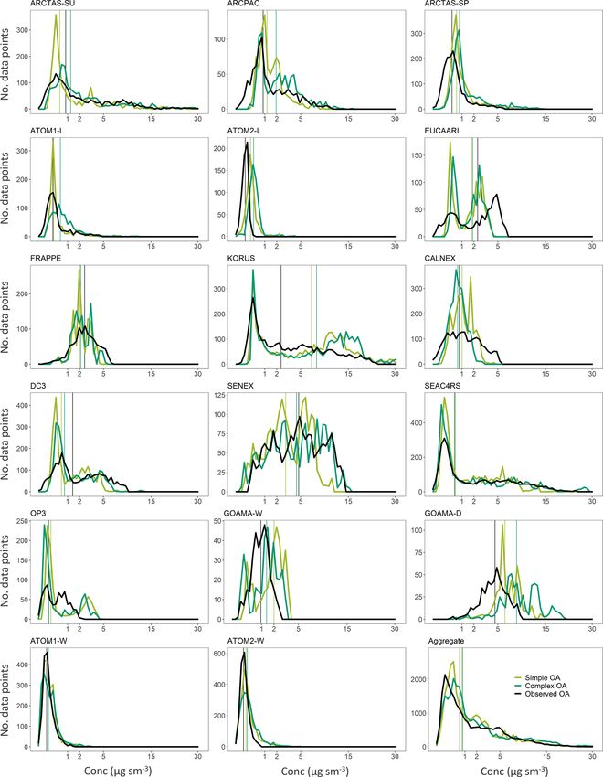
S. J. Pai et al.: An evaluation of global organic aerosol schemes using airborne observations                             2639

the various emission inventories and chemical mechanisms.        scheme represents a more detailed, recently updated treat-
Here, we use a top-down approach, leveraging a suite of          ment of organic aerosol in the atmosphere based on numer-
15 aircraft campaigns to evaluate the two different organic      ous laboratory studies and an explicit chemical mechanism
aerosol schemes implemented within the standard GEOS-            for the oxidation of isoprene. The simple scheme is designed
Chem chemical transport model in order to assess their rela-     to serve as a computationally efficient alternative for approx-
tive strengths and weaknesses over a wide range of chemical      imating tropospheric OA concentrations without attempting
and spatial regimes.                                             to model the formation and fate of the various aerosol species
                                                                 mechanistically and without explicit thermodynamic parti-
                                                                 tioning. We note that the simple scheme was developed in-
2     Model description                                          dependently from the complex scheme and should not be re-
                                                                 garded as a reduced version of the complex scheme. These
We use the chemical transport model GEOS-Chem (http:             schemes are described below and are graphically illustrated
//www.geos-chem.org, last access: 5 January 2019) to sim-        in Fig. 1.
ulate organic aerosol mass concentrations along the flight          The simple scheme treats all organic aerosol as non-
tracks of a suite of airborne campaigns described in Sect. 3.    volatile. The POA consists of a hydrophobic “emitted” com-
In order to contrast the different approaches to modeling or-    ponent (EPOA) with an assumed organic-mass-to-organic-
ganic aerosol and its precursors in the atmosphere, we per-      carbon (OM : OC) ratio of 1.4 and a hydrophilic “oxy-
form a series of simulations from 2008 to 2017 using two         genated” component (OPOA) with an assumed OM : OC
distinct model schemes that vary based on their treatment of     ratio of 2.1. Of the organic carbon emitted from primary
organic aerosol (see Sect. 2.1 and Table S1 in the Supple-       sources, 50 % is assumed to be hydrophilic (OPOA) to simu-
ment).                                                           late the near-field oxidation of EPOA. The atmospheric aging
   These       simulations      were      performed       with   of EPOA is modeled by its conversion to hydrophilic aerosol
the       GEOS-Chem           model       version       12.1.1   (OPOA) with an atmospheric lifetime of 1.15 d, with no ex-
(https://doi.org/10.5281/zenodo.2249246;         International   plicit dependence on local oxidant levels (Chin et al., 2002;
GEOS-Chem User Community, 2018) with a horizontal res-           Cooke et al., 1999). The EPOA and OPOA species are rep-
olution of 2◦ × 2.5◦ and 47 vertical hybrid-sigma levels that    resented within the GEOS-Chem model using the variable
extend from the surface to the lower stratosphere. A series      names OCPO and OCPI, respectively. In addition, GEOS-
of nested simulations, over North America and Asia, were         Chem includes an online emission parameterization for sub-
performed at a higher spatial resolution of 0.5◦ × 0.625◦        micron non-volatile marine primary organic aerosol (MPOA)
using boundary conditions from the 2◦ × 2.5◦ global run.         as described in Gantt et al. (2015). The marine POA is emit-
The model is driven by the MERRA-2 assimilated mete-             ted as hydrophobic (M-EPOA) and is aged in the atmosphere
orological product from the NASA Global Modeling and             by its conversion to hydrophilic aerosol (M-OPOA), with the
Assimilation Office (GMAO) with a transport time step            same 1.15 d lifetime. For the purpose of this study, the hy-
of 10 min as recommended by Philip et al. (2016). The            drophobic and hydrophilic components have been lumped
model includes a coupled treatment of HOx –NOx –VOC–O3           together under the MPOA moniker.
chemistry (Mao et al., 2013; Travis et al., 2016; Chan Miller       The simple scheme uses a lumped SOA product (SOAS)
et al., 2017) with integrated Cl–Br–I chemistry (Sherwen et      with a molecular weight of 150 g mol−1 and an SOA pre-
al., 2016) and uses a bulk aerosol scheme with fixed log-        cursor (SOAP) that is emitted from biogenic, pyrogenic and
normal modes (Martin et al., 2003). GEOS-Chem simulates          anthropogenic sources with fixed OA yields. For biogenic
sulfate aerosol (Park, 2004), sea salt (Jaeglé et al., 2011),    SOA, a 3 % yield from isoprene (Kim et al., 2015) and 10 %
black carbon (Park et al., 2003) and mineral dust (Fairlie       yield from both monoterpenes and sesquiterpenes (Chin et
et al., 2007; Ridley et al., 2012). Ammonium and nitrate         al., 2002) is assumed. SOA precursor emissions from com-
thermodynamics are described using the ISORROPIA II              bustion sources are estimated using CO emissions as a proxy,
model (Fountoukis and Nenes, 2007). Deposition losses are        with a 1.3 % scaled co-emission of SOAP from fire and bio-
dictated by aerosol and gas dry deposition to surfaces based     fuel CO and a 6.9 % SOAP co-emission from fossil fuel
on a resistor-in-series scheme (Wesely, 1989; Zhang et al.,      CO (Cubison et al., 2011; Hayes et al., 2015; Kim et al.,
2001) and wet deposition from scavenging by rainfall and         2015). For biogenic SOA from isoprene, monoterpenes and
moist convective cloud updrafts (Amos et al., 2012; Jacob et     sesquiterpenes, 50 % is emitted directly as SOAS to account
al., 2000; Liu et al., 2001). More details on the deposition     for the near-field formation of secondary organic aerosol.
schemes are provided in the Supplement.                          The SOAP converts to SOAS based on a first-order rate con-
                                                                 stant with a lifetime of 1 d as it is transported through the
2.1    Organic aerosol simulations                               troposphere (Fig. 1).
                                                                    For the purpose of this study, the default simple scheme in
This study evaluates the two standard organic aerosol            GEOS-Chem was modified to individually simulate 14 OA
schemes within the GEOS-Chem model. The complex                  lumped model tracers from anthropogenic, biogenic, marine

www.atmos-chem-phys.net/20/2637/2020/                                             Atmos. Chem. Phys., 20, 2637–2665, 2020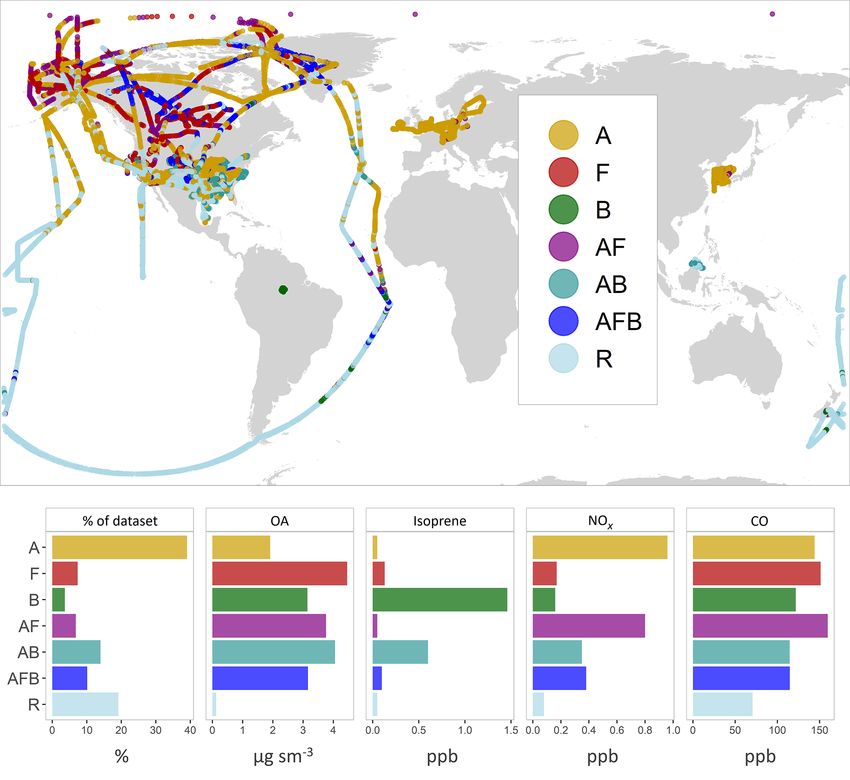
2640                            S. J. Pai et al.: An evaluation of global organic aerosol schemes using airborne observations

Figure 1. A graphical overview of the two organic aerosol model schemes in GEOS-Chem. TERP denotes monoterpenes and sesquiter-
penes. Pyrogenic VOCs (FVOCs) denote the various volatile and semi-volatile organic compounds emitted from fires, while anthropogenic
VOCs (AVOCs) are comprised of benzene, toluene, xylene and various intermediate-volatility organic compounds that are modeled us-
ing naphthalene as a proxy. OPOA∗ is sometimes classified as secondary organic aerosol from SVOCs. MPOA∗∗ denotes lumped marine
POA consisting of both fresh (M-EPOA) and oxidized (M-OPOA) components. Species in orange contribute to OA; images modified from
https://openclipart.org/ (last access: 11 January 2018) and https://publicdomainvectors.org/ (last access: 5 December 2019). See Sect. 2.1 in
the text for details.

and pyrogenic sources. These consisted of six POA tracers,               precursors, while classifying the OA resulting from the ox-
four SOA tracers and four SOA precursor tracers, allowing                idation of primary organic compounds as OPOA, in order
for the independent adjustment of parameters such as emis-               to be consistent with previous model studies using GEOS-
sion rates, yields, chemical lifetimes and deposition rates, en-         Chem (Pye et al., 2010). Model EPOG emissions are based
abling a robust testing of various sensitivities and OA source           on the EPOA inventories used in the simple scheme and have
attributions.                                                            been scaled up by 27 % to account for semi-volatile organic
    The complex scheme, based primarily on Pye et al. (2010)             matter emitted in the gas phase (Pye et al., 2010; Schauer et
and Marais et al. (2016), is graphically described in Fig. 1.            al., 2001). As in the simple scheme, the EPOA and OPOA
The primary organics are treated as semi-volatile and al-                are assumed to have an OM : OC ratio of 1.4 and 2.1, respec-
lowed to reversibly partition between the aerosol (EPOA)                 tively. The complex scheme also includes the non-volatile
and gas (EPOG) phase using a two-product reversible par-                 MPOA simulation as described above.
titioning model while simultaneously undergoing oxidation                   SOA formation from anthropogenic, pyrogenic and se-
with OH in the gas phase to form oxidized primary organic                lect biogenic precursors is based on the VBS outlined in
gases (OPOGs) that, in turn, reversibly partition to oxidized            Pye et al. (2010) that oxidizes gas-phase SOA precursors
primary organic aerosols (OPOAs). Primary semi-volatile or-              (with oxidants – OH, O3 ) to form alkyl peroxy (RO2 ) rad-
ganic vapors that are oxidized to form lower-volatility prod-            icals that react with either HO2 or NO. The SOA formed
ucts are sometimes classified as secondary organic aerosol               from these second-generation products depends on the NOx
(Murphy et al., 2014). However, for the purpose of this study,           regime – with high and low NOx yields and partitioning co-
we define SOA as being formed exclusively from volatile                  efficients based on experimental fits from laboratory stud-

Atmos. Chem. Phys., 20, 2637–2665, 2020                                                    www.atmos-chem-phys.net/20/2637/2020/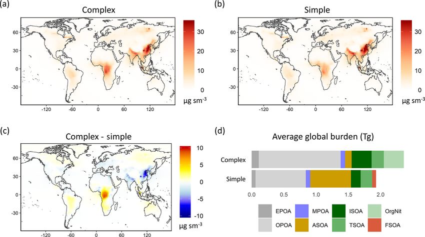
S. J. Pai et al.: An evaluation of global organic aerosol schemes using airborne observations                               2641

ies. The resulting products are classified into two categories   Table 1. Global annual mean emissions of SOA precursors and rel-
based on the origins of their precursors, anthropogenic SOA      evant species used in the GEOS-Chem simulation for the year 2013.
(ASOA; formed from the oxidation of light aromatic com-
pounds) and terpene SOA (TSOA; formed from the oxidation                    Species                       Annual global
of monoterpenes and sesquiterpenes), that dynamically parti-                                         emissions (Tg yr−1 )
tion between the aerosol and gas phases based on their satu-                Total aromatics                         25.6
ration vapor pressures and ambient aerosol concentrations.                     Anthropogenic                        23.5
Aerosol formed from intermediate-volatility organic com-                       Pyrogenic                             2.1
pounds (IVOCs) is modeled using naphthalene as a proxy
                                                                            IVOCs                                   5.43
that, when oxidized, contributes to the ASOA lumped prod-
uct. A comprehensive overview of the VBS scheme can be                      Isoprene                               385.3
found in Pye et al. (2010).                                                 Terpenes                               153.6
   The complex scheme builds on this VBS framework by
incorporating aerosol formed irreversibly from the aqueous-                 Total CO                               891.2
phase reactive uptake of isoprene (Marais et al., 2016) and                    Anthropogenic                       593.0
the formation of organo-nitrates (Org-Nit) from both iso-                      Pyrogenic                           298.2
prene and monoterpene precursors (denoted in Fig. 1) based                  Total NOx                              111.7
on work by Fisher et al. (2016). These mechanisms replace                      Anthropogenic                        70.7
the “pure-VBS” treatment of isoprene SOA (ISOA) and or-                        Pyrogenic                            12.1
ganic nitrates (formed from the oxidation of isoprene and                      Lightning                            12.7
monoterpenes by NO3 ) from Pye et al. (2010). The total                        Soil and fertilizer                  16.2
organic aerosol loadings in the complex scheme are thus
comprised of the EPOA, OPOA, ASOA and TSOA species
in addition to the various products resulting from the iso-      the same approach as Pye and Seinfeld (2010). These emis-
prene and monoterpene organo-nitrate oxidation pathways          sions are overwritten with regional inventories when avail-
(organic nitrates from isoprene and monoterpene precursors,      able, such as the National Emissions Inventory (NEI 2011)
aerosol-phase glyoxal, methylglyoxal, isoprene epoxydiols        for the US (as described by Travis et al., 2016), the Big Bend
– IEPOX, C4 epoxides, organo-nitrate hydrolysis products,        Regional Aerosol and Visibility Observational (BRAVO) in-
second-generation hydroxy-nitrates, and low-volatility non-      ventory for Mexico (Kuhns et al., 2005), the Criteria Air
IEPOX products of isoprene hydroxy hydroperoxide oxida-          Contaminants (CAC) inventory for Canada (https://www.
tion), lumped here as ISOA and Org-Nit. ISOA and Org-Nit         canada.ca/en/environment-climate-change.html, last access:
are generated exclusively through the aqueous uptake path-       5 December 2019), the European Monitoring and Evalua-
way and do not include any “nonaqueous” OA. The model            tion Programme (EMEP) inventory for Europe (http://www.
does not explicitly consider cloud processing of SOA. More       emep.int/, last access: 5 December 2019), the Diffuse and In-
information on the treatment of OA in the complex scheme         efficient Combustion Emissions (DICE) inventory for Africa
can be found in the Supplement.                                  (Marais and Wiedinmyer, 2016) and the MIX inventory for
   In order to conduct a comparison with a VBS treatment of      Asian emissions (Li et al., 2017). In addition to the anthro-
isoprene SOA (as described in Pye et al., 2010), an analysis     pogenic and pyrogenic inventories listed above, nitrogen ox-
was also conducted with the isoprene SOA forming exclu-          ides are also emitted from lightning (Murray et al., 2012; Ott
sively through the VBS (referred to here as pure VBS).           et al., 2010), soil (Hudman et al., 2012) and ship (Holmes
                                                                 et al., 2014) sources. Biogenic emissions for isoprene and
2.2   Emissions                                                  terpene species in GEOS-Chem are based on the coupled
                                                                 ecosystem emissions model MEGAN (Model of Emissions
Global annual mean emissions of key species for a single         of Gases and Aerosols from Nature) v2.1 (Guenther et al.,
simulation year (2013) are shown in Table 1. The correspond-     2012). All emissions are managed via the Harvard–NASA
ing emissions (and atmospheric sources) for OA species are       Emissions Component (HEMCO) module (Keller et al.,
shown in Table 2. Year-specific pyrogenic emissions are          2014). We note that given the interannual variability in emis-
simulated at a 3 h resolution from the GFED4s satellite-         sions, particularly from fires, the emissions for years other
derived global fire emissions database (van der Werf et al.,     than 2013 may differ somewhat from the values shown in
2017). Global anthropogenic emissions follow the Commu-          Tables 1 and 2.
nity Emissions Data System (CEDS) inventory (Hoesly et al.,         In the simple scheme, 50 % of the primary OA is emitted
2018). Anthropogenic IVOC emissions are estimated using          as EPOA and 50 % is emitted as OPOA to approximate the
naphthalene as a proxy (see the Supplement for more infor-       near-field aging of EPOA. Total OC emissions are 31.2 Tg C.
mation), which is assumed to have the same spatial distribu-     Given the OC : OM ratios of 1.4 and 2.1 assumed for EPOA
tion as benzene and is scaled from the CEDS inventory using      and OPOA, respectively, total POA emissions in the sim-

www.atmos-chem-phys.net/20/2637/2020/                                              Atmos. Chem. Phys., 20, 2637–2665, 2020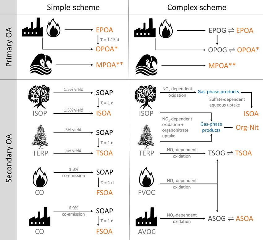
2642                                     S. J. Pai et al.: An evaluation of global organic aerosol schemes using airborne observations

Table 2. Annual mean simulated global source, burden, lifetime (against physical deposition), and wet and dry deposition rates for the
individual OA species averaged over 2013 for the complex and simple schemes.

                                                               Complex                                                                     Simple
                                     Source       Burden       Lifetime       Dry dep.       Wet dep.         Source        Burden      Lifetime       Dry dep.        Wet dep.
                                  (Tg yr −1 )       (Tg)             (d)     (Tg yr−1 )     (Tg yr−1 )      (Tg yr−1 )        (Tg)            (d)     (Tg yr−1 )      (Tg yr−1 )
 Total POA                             87.3c         1.46            6.1           14.7            72.6           73.8c        0.92            4.6           13.2           60.6
    Emitted POA                        55.4d         0.11           11.5            2.1             1.4            21.8        0.06            7.8            1.4            1.4
    Marine EPOA                          7.0         0.02            4.3            0.9             0.8             7.0        0.02            4.3            0.9            0.8
    Oxygenated POAa                    74.1c         1.27            6.3           10.2            63.9           61.3c        0.78            4.6            9.4           51.9
    Marine OPOAa                        8.0c         0.06            2.8            1.5             6.5            8.0c        0.06            2.8            1.5            6.5
 Total SOA                              62.9c        0.91            5.3             7.3           55.6           71.7         1.02            5.2            9.4           62.2
    Anthropogenic SOA                    4.6c        0.10            7.9             0.6            4.0           41.0         0.63            5.6            6.2           34.8
    Terpene SOA                         13.1c        0.19            5.3             1.5           11.6           15.2         0.18            4.3            1.6           13.6
    Isoprene SOA                        22.2c        0.31            5.1             2.3           19.9           11.6         0.15            4.7            1.1           10.4
    Organic nitrates                    23.0c        0.31            4.9             2.9           20.1              –            –              –              –              –
    Pyrogenic SOA                           –           –              –               –              –            3.9         0.06            5.7            0.5            3.4
 Total OOAb                           145.0c         2.24            5.6           19.0          126.0          140.9c         1.86            4.8           20.3          120.6
 Total OA                             150.1c         2.37            5.8           21.9          128.2          145.3c         1.94            4.9           22.6          122.8
a SVOCs from primary sources that are oxidized in the atmosphere, sometimes classified as SOA. b OOA (oxygenated organic aerosol) = OPOA + M-OPOA + SOA.
c Calculated based on a steady-state assumption with depositional losses in order to account for atmospheric formation. The total POA source is not the direct sum of the individual
POA sources since a significant fraction of EPOA and MPOA forms OPOA and M-OPOA, respectively. See Sect. 2.2 for emissions totals and more information. d Primary organic
emissions in the complex scheme are in the gas phase (EPOG), while primary organic emissions in the simple scheme are in the form of non-volatile particulate. An OM : OC
ratio of 1.4 is assumed for the EPOG and EPOA species, while an OM : OC ratio of 2.1 is assumed for the OPOA species.

ple scheme are 21.8 Tg EPOA and 32.8 Tg OPOA for a to-                                       normalized mean bias is calculated using Eq. (2). A positive
tal annual POA emission of 54.6 Tg. We note that OPOA                                        NMB indicates that the model is biased high on average and
emissions in the simple scheme are a subset of the sources                                   vice versa.
listed in Table 2 since they do not include atmospheric for-
mation through the oxidative aging of EPOA. In the com-                                      Coefficient of determination
plex scheme, all POA is emitted as gas-phase EPOG af-                                                   Residual sum of squares
ter scaling the same inventory used in the simple scheme                                      R2 = 1 −                                                                         (1)
                                                                                                             Total sum of squares
by 27 % to account for the extra gas-phase material. To-
tal primary emissions in the complex scheme are thus ex-                                     Normalized mean bias
clusively from EPOG gas-phase emissions and amount to
                                                                                                             n
55.4 Tg yr−1 . Both schemes emit an additional 7.0 Tg yr−1                                                   P
                                                                                                                  (model − observation)
of OA from marine sources. The simple scheme also di-                                                         1
                                                                                             (NMB) =                                                                           (2)
rectly emits 71.7 Tg yr−1 of SOA (in the form of SOAS                                                               n
                                                                                                                    P
and SOAP), over half of which comes from anthropogenic                                                                   (observation)
                                                                                                                     1
sources. The total OA source (POA + SOA; includes direct
emissions and atmospheric formation) in both the complex
and simple schemes (150.1 and 145.3 Tg yr−1 , respectively;                                  3    Description of observations
Table 2) is greater than the ensemble median OA source
of around 100 Tg yr−1 calculated by Tsigaridis et al. (2014)                                 For the purposes of evaluating the GEOS-Chem model, we
across a set of various global models.                                                       focus on airborne data that provide regional 3-D sampling
                                                                                             and reduce the challenges associated with model representa-
2.3     Model evaluation                                                                     tion error at single sites. We further define a set of observa-
                                                                                             tions that make use of a single measurement technique, are
Two primary metrics have been used through this study to                                     publicly accessible and do not extend beyond the last decade.
evaluate model performance compared to ambient observa-                                      The resulting observations are from 15 aircraft campaigns
tions (see Sect. 3) – the coefficient of determination (R 2 ) and                            conducted between 2008 and 2017 and cover a wide range of
the normalized mean bias (NMB). The coefficient of deter-                                    geographic locations and chemical regimes. Table 3 provides
mination is defined by the regression fit using Eq. (1) and can                              a brief overview of the various campaigns included here, and
be interpreted as the proportion of the variance in the obser-                               Fig. 2 shows the spatial extent of the individual flight tracks.
vational data that is accurately captured by the model. The                                  Aerosol concentrations were measured using aerosol mass

Atmos. Chem. Phys., 20, 2637–2665, 2020                                                                              www.atmos-chem-phys.net/20/2637/2020/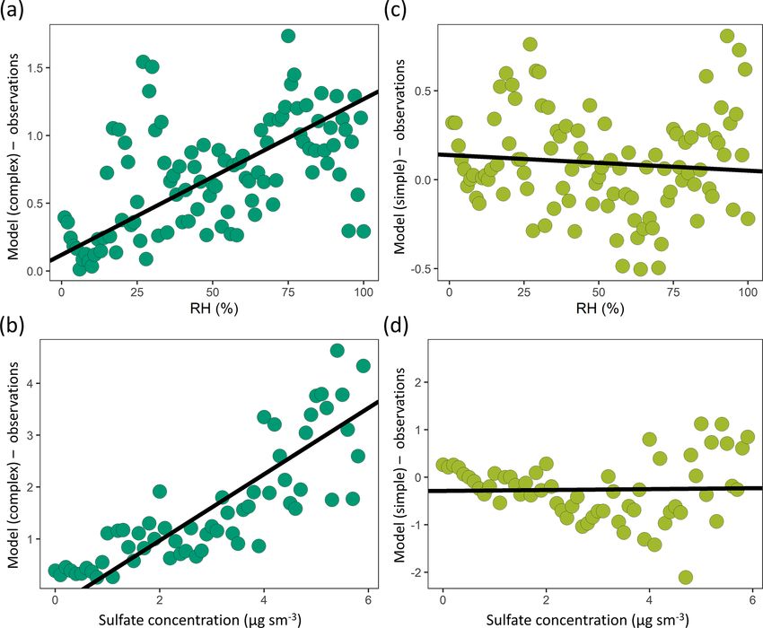
S. J. Pai et al.: An evaluation of global organic aerosol schemes using airborne observations                                     2643

                                                                        observed mean, medians and standard deviations across the
                                                                        different campaigns (Table 3, Fig. S1). The campaigns are
                                                                        also influenced by different OA sources depending on their
                                                                        sampling region. The EUCAARI campaign over western Eu-
                                                                        rope (Morgan et al., 2010), KORUS-AQ over the Korean
                                                                        Peninsula (Nault et al., 2018), CalNex over California (Ryer-
                                                                        son et al., 2013), and DC3 (Barth et al., 2014) and FRAPPE
                                                                        over the central US (Dingle et al., 2016) sample over regions
                                                                        that are heavily influenced by anthropogenic emissions. In
                                                                        contrast, the GoAmazon campaigns during the wet and dry
                                                                        seasons (Martin et al., 2016; Shilling et al., 2018) over the
                                                                        Manaus region in the Amazon and the OP3 campaign (He-
Figure 2. Location of flight tracks for the airborne field campaigns.   witt et al., 2010) over equatorial forests in southeast Asia are
                                                                        heavily influenced by biogenic emissions, although the GoA-
                                                                        mazon campaign in the dry season is also strongly influenced
spectrometers (AMSs) (Jayne et al., 2000; Canagaratna et al.,           by biomass burning. Additionally, data from both seasons of
2007) with small variations in the instrumentation and air-             the GoAmazon campaign are influenced by anthropogenic
craft inlet configurations between the different campaigns (as          urban outflow from Manaus (Shilling et al., 2018). Cam-
referenced in Table 3). The AMS measures submicron non-                 paigns like SENEX (Warneke et al., 2016) and SEAC4RS
refractory dry aerosol mass and is estimated to have an un-             (Toon et al., 2016) that conducted measurements over the
certainty of 34 %–38 %, depending on the species (Bahreini              southeast US are influenced by both anthropogenic and bio-
et al., 2009). All concentration measurements in this study             genic emissions, while the ARCPAC campaign (Brock et al.,
have been converted to standard conditions of temperature               2011) during the spring and the ARCTAS (Jacob et al., 2010)
and pressure (STP: 273 K, 1 atm; µg sm−3 ). In addition to or-          campaign during the spring and summer over the north-
ganic aerosol mass loadings, concentrations of other species,           ern latitudes are strongly influenced by pyrogenic emissions
such as nitrogen oxides, carbon monoxide, isoprene and sul-             from forest fires (particularly during the summer) and aged
fate, are used in this study to validate chemical regimes (see          anthropogenic and biogenic emissions over the Arctic region.
Sect. 4.2). Table S2 provides an overview of the instrumen-             The KORUS-AQ campaign also includes a short deploy-
tation and associated primary investigators for the organic             ment over California. However, for the purpose of this study,
aerosol and trace gas observations. Environmental and me-               we restrict observations from this campaign to those over
teorological measurements such as temperature and relative              the Korean Peninsula. Lastly, the dataset includes measure-
humidity are also used in the analysis.                                 ments from the ATom-1 and ATom-2 campaigns (Wofsy et
   Observations are gridded to the GEOS-Chem model reso-                al., 2018). We divide the ATom campaigns into two datasets
lution of 2◦ × 2.5◦ (or alternatively to 0.5◦ × 0.625◦ for com-         using a land mask in order to separate the observations of re-
parisons with nested simulations) and are averaged over the             mote, well-mixed air masses over the Atlantic and the Pacific
model time step of 10 min in cases in which multiple obser-             from near-source measurements over North America.
vations were conducted within the span of a single time step               Figure 3 demonstrates that organic aerosol accounts for
(see the Supplement for more details on model sampling). In             a significant portion (52 % on average) of the total non-
order to limit the impact of localized plumes, in particular            refractory aerosol mass loadings measured by AMS across
from fires, we filter the observations to remove concentra-             all of the campaigns. The GoAmazon measurements during
tions over the 97th percentile for each campaign, eliminating           the dry season have the highest contribution of OA to the
measurements that can often exceed 500 µg sm−3 . This en-               total submicron aerosol loading (77 %), while the ARCTAS
ables a more fair comparison with the model by disregarding             campaign during the spring has the lowest OA contribution
the impact of sub-grid features that cannot be reproduced by            of any campaign (31 %).
an Eulerian model (Rastigejev et al., 2010). Following the av-
eraging process, we obtain a merged dataset of over 25 000
unique points, with a broad spatial extent (Fig. 2) covering            4     Results and discussion
a variety of chemical regimes representing anthropogenic,
pyrogenic, biogenic and remote environments. Despite the                4.1    Simulated OA budget
large temporal range of the observational dataset, most of the
campaigns analyzed in this study were conducted during the              Figure 4 shows the global annual mean simulated surface
spring and summer seasons, limiting the ability to perform a            OA concentrations and global annual mean burdens using
seasonal analysis.                                                      the simple and complex schemes for the year 2013 (bur-
   Based on the proximity to emission sources and exposure              den numbers are provided in Table 2). The complex scheme
to long-range pollutants, there is significant variation in the         simulates a larger annual mean OA burden than the simple

www.atmos-chem-phys.net/20/2637/2020/                                                    Atmos. Chem. Phys., 20, 2637–2665, 2020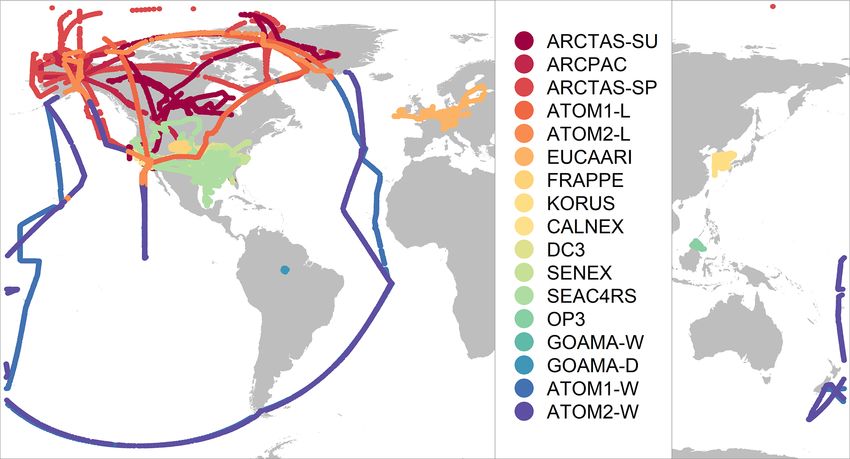
2644                             S. J. Pai et al.: An evaluation of global organic aerosol schemes using airborne observations

Table 3. Aircraft measurements of organic aerosol used in this analysis. The statistical metrics for OA provided here (mean, median, standard
deviation) are based on filtered data for each campaign (as discussed in the text; units: µg m−3 ).

 Campaign                  Dates (UTC, mm/dd)                     Region                   Abbreviation    Measurement      Mean, median,
                                                                                                           technique                  SD
 ARCPAC                    2008 spring (03/29–04/24)              Arctic, North America    –               C-ToF-AMS           1.9, 0.9, 2.1
 (Brock et al., 2011)
 ARCTAS                    2008 spring (04/01–04/20)              Arctic, North America    ARCTAS-SP       HR-ToF-AMS          0.7, 0.4, 0.9
 (Jacob et al., 2010)
 ARCTAS                    2008 summer (06/18–07/13)              Arctic, North America    ARCTAS-SU       HR-ToF-AMS          3.2, 0.9, 5.1
 (Jacob et al., 2010)
 EUCAARI                   2008 spring (05/06–05/22)              Northwest Europe         –               C-ToF-AMS           2.5, 2.4, 2.0
 (Morgan et al., 2010)
 OP3                       2008 summer (07/10–07/20)              Borneo                   –               C-ToF-AMS           0.4, 0.1, 0.5
 (Hewitt et al., 2010)
 CalNex                    2010 spring and summer (04/30–06/22)   Southwest US             –               C-ToF-AMS           1.3, 0.8, 1.4
 (Ryerson et al., 2013)
 DC3                       2012 spring and summer (05/18–06/23)   Central US               –               HR-ToF-AMS          2.5, 1.4, 2.4
 (Barth et al., 2014)
 SENEX                     2013 summer (06/03–07/10)              Southeast US             –               C-ToF-AMS           5.3, 4.7, 3.7
 (Warneke et al., 2016)
 SEAC4RS                   2013 summer and fall (08/06–09/24)     Southeast, west US       –               HR-ToF-AMS          3.2, 0.6, 4.6
 (Toon et al., 2016)
 GoAmazon                  2014 wet season (02/22–03/23)          Amazon                   GOAMA-W         HR-ToF-AMS          1.0, 0.9, 0.6
 (Shilling et al., 2018)
 FRAPPE                    2014 summer (07/26–08/19)              Central US               –               C-ToF-mAMS          2.7, 2.5, 1.4
 (Dingle et al., 2016)
 GoAmazon                  2014 dry season (09/06–10/04)          Amazon                   GOAMA-D         HR-ToF-AMS          4.6, 4.6, 1.8
 (Shilling et al., 2018)
 KORUS-AQ                  2016 spring and summer (05/03–06/10)   South Korea              KORUS           HR-ToF-AMS          4.8, 2.4, 5.5
 (Nault et al., 2018)
 ATom                      2016 summer (07/29–08/20)              Remote ocean             ATOM1-W         HR-ToF-AMS          0.1, 0.1, 0.2
 (Wofsy et al., 2018)                                             North America            ATOM1-L                             0.5, 0.2, 0.8
 ATom                      2017 spring (01/26–02/21)              Remote ocean             ATOM2-W         HR-ToF-AMS          0.1, 0.1, 0.1
 (Wofsy et al., 2018)                                             North America            ATOM2-L                             0.1, 0.1, 0.1
 Aggregate                                                                                                                     2.4, 0.7, 3.6

scheme (2.37 Tg compared to 1.94 Tg). This is largely due to             typical AMS measurements (Jimenez et al., 2009). Conse-
the scaled emissions of the primary organic gases in the com-            quently, 94.7 % of the global OA burden in the complex
plex scheme (greater by a factor of 27 %) as well as the semi-           scheme is oxygenated organic aerosol (OOA = OPOA + M-
volatile treatment of the EPOA/EPOG and OPOA/OPOG                        OPOA + SOA; Table 2). Similarly, 91.7 % of the total POA
species, which substantially extends their tropospheric resi-            burden and 96.1 % of the total OA burden are oxygenated in
dence time due to the longer lifetime of the gas-phase compo-            the simple scheme.
nent in the boundary layer. As a result, the complex scheme                 Both the complex and simple schemes simulate compa-
simulates a larger POA burden (EPOA + OPOA + MPOA)                       rable global SOA burdens (0.91 and 1.02 Tg, respectively).
of 1.46 Tg, compared to 0.92 Tg POA in the simple scheme.                However, the complex scheme produces more isoprene-
The majority (91.4 %) of the POA in the complex scheme                   derived SOA (ISOA) and biogenic organo-nitrates (Org-Nit)
consists of oxidized POA and oxidized MPOA (M-OPOA)                      than the simple scheme (Fig. 4d), particularly over areas
that, given its aged and chemically processed nature, is of-             with elevated isoprene and anthropogenic sulfate concentra-
ten indistinguishable from secondary organic aerosol with                tions (such as the southeast US and southeast Asia) since

Atmos. Chem. Phys., 20, 2637–2665, 2020                                                    www.atmos-chem-phys.net/20/2637/2020/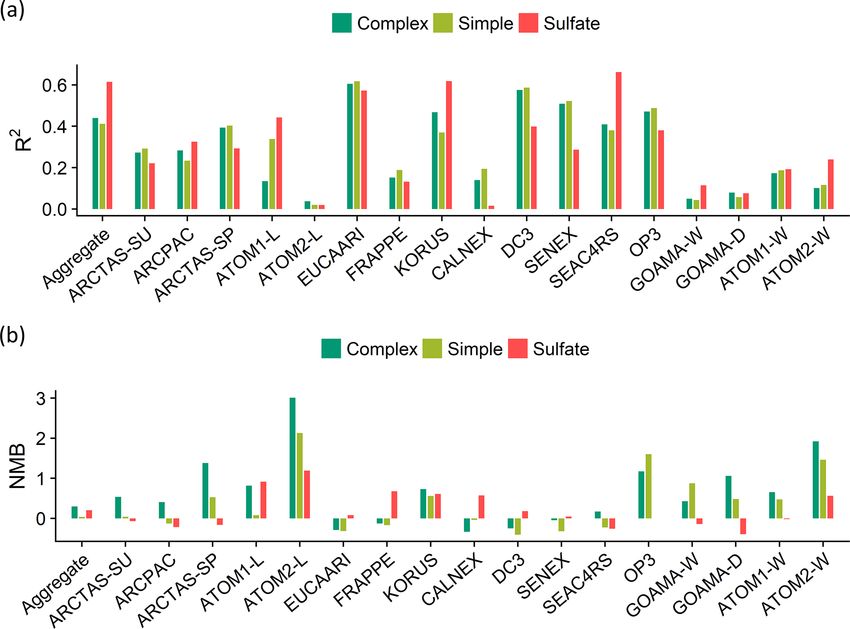
S. J. Pai et al.: An evaluation of global organic aerosol schemes using airborne observations                                             2645

Figure 3. The percentage contribution of organic aerosol by mass to the total observed non-refractory mass concentrations measured by
the AMS; organized by campaign. This includes aerosol mass from organic aerosol, sulfate, nitrate and ammonium. Campaigns are broadly
organized based largely on model-characterized source influence. However, as noted in the text, this characterization is often not indicative of
the true sampling profile. For instance, the GoAmazon campaigns sampled heavily from fire and anthropogenic sources in addition to being
strongly influenced by biogenic sources.

Figure 4. Global map of simulated OA surface concentrations in 2013 for the (a) complex and (b) simple schemes; panel (c) illustrates the
difference in OA surface loadings between the complex and simple schemes. Panel (d) displays the total global burden for the individual OA
species from both schemes averaged over 2013. Refer to Sect. 3 for details on model sampling and averaging.

the ISOA formation is acid-catalyzed. The explicit aque-                  schemes have similar terpene-derived SOA (TSOA) burdens
ous uptake mechanism for the isoprene-derived SOA prod-                   at 0.19 and 0.18 Tg, respectively (Table 2).
ucts also results in substantially larger global isoprene SOA                Anthropogenic SOA (ASOA) is a particularly important
burdens (0.31 Tg) when compared to the pure-VBS treat-                    global OA source in the simple scheme, accounting for al-
ment of isoprene-derived SOA that simulates an annually                   most a third of the total OA burden. The simple scheme,
averaged ISOA burden of 0.12 Tg. This is consistent with                  with its near-field formation of SOA proportional to an-
other comparisons that have shown that the VBS treatment in               thropogenic CO emissions, simulates a substantially larger
GEOS-Chem underpredicts observed ISOA concentrations                      ASOA burden than the complex scheme (0.63 vs. 0.10 Tg;
compared to the complex treatment (Jo et al., 2019). De-                  Table 2), particularly over industrialized regions in Asia
spite the different treatments, both the complex and simple               (Fig. 4c). Previous studies that have constrained global

www.atmos-chem-phys.net/20/2637/2020/                                                        Atmos. Chem. Phys., 20, 2637–2665, 2020
2646                         S. J. Pai et al.: An evaluation of global organic aerosol schemes using airborne observations

SOA burdens using observed mass loadings have proposed           who calculated an ensemble mean POA lifetime of approxi-
a missing model SOA source over anthropogenic regions            mately 5 d. SOA lifetimes from this study are lower than the
(Spracklen et al., 2011), as have recent regional studies        ensemble mean of 8 d calculated by Tsigaridis et al. (2014).
(Schroder et al., 2018; Shah et al., 2019). The simple scheme    The range in aerosol lifetimes can be attributed to several
appears to capture a greater fraction of this missing burden.    different factors. The hydrophobic nature of EPOA leads to
However, we note that ASOA yields in the simple scheme           longer lifetimes against wet deposition since the particles are
are based on a lumped parameterization over the Los Ange-        unaffected by rainout. The spatial distribution of the differ-
les basin (Hayes et al., 2015) and might not be representa-      ent aerosol types also plays an important role in determin-
tive of global yields across different chemical regimes. The     ing their lifetimes, with species emitted over marine–tropical
global ASOA burden of 0.63 Tg is 4 times greater than the        regions experiencing a higher likelihood of being deposited
ASOA burden proposed by Spracklen et al. (2011), but it is       via wet deposition than aerosol over drier regions. Surface
well within the “anthropogenically controlled” SOA burden        land types also affect dry deposition velocities, impacting
proposed by the same study. This suggests that the simple        aerosol lifetimes. In addition, there is a marked difference
parametrization in its current form might unintentionally rep-   in lifetimes between the semi-volatile species in the complex
resent some anthropogenically controlled biogenic SOA. Ad-       scheme and non-volatile species in the simple scheme. Due
ditionally, while the simple scheme includes separate SOA        to the temperature-dependent partitioning, the semi-volatile
yield parameters for fossil fuel and biofuel combustion, the     aerosol species are often in the gas phase in the warmer parts
emissions inventories used in this study do not always explic-   of the troposphere and are advected to higher altitudes before
itly differentiate between the two sources. As a consequence,    they partition to aerosol. The non-volatile species do not sim-
biofuel is often lumped together with fossil fuel CO, poten-     ulate this process and are more likely to be deposited before
tially leading to an overestimate in ASOA yields from biofuel    they can be transported to higher altitudes.
emissions.
   Pye and Seinfeld (2010) performed a similar analysis of       4.2   Regime analysis
tropospheric OA burdens using a semi-volatile POA treat-
ment and a pure-VBS treatment of SOA (i.e., all SOA treated      We use the observations from the 15 field campaigns de-
in the VBS, including isoprene) with the GEOS-Chem model         scribed in Sect. 3 as a single coherent dataset. Given the wide
(v8.01.04). Their model simulated 0.03 Tg EPOA, 0.81 Tg          range of chemical regimes sampled by the various field cam-
OPOA and 0.80 Tg SOA compared to 0.11 Tg EPOA,                   paigns, a method for classifying the observations is needed to
1.27 Tg OPOA and 0.91 Tg SOA for the complex scheme              better inform the model–measurement comparisons. While
and 0.06 Tg EPOA, 0.78 Tg OPOA and 1.02 Tg SOA for the           the chemical composition of the observed OA can provide
simple scheme in this study. When compared to an analy-          some insight into source types or aging, a comprehensive
sis of organic aerosol loadings from 31 different chemical       classification is not possible using only the observations, re-
transport and general circulation models (Tsigaridis et al.,     quiring that we rely on the model for such a segmentation.
2014), the primary OA burden from the complex scheme             In this analysis, we use the relative dominance of the differ-
(EPOA + MPOA + OPOA) is substantially higher than most           ent OA species within the GEOS-Chem simple scheme sim-
of the models surveyed, while the SOA burden falls below         ulation to classify the measurements into different regimes
the mean but above the median of the distribution. The sim-      (described in Table S3 in the Supplement). The sorting algo-
ple scheme, with a much smaller POA burden, is approx-           rithm weights the relative importance of the three OA source
imately on par with the Tsigaridis et al. (2014) ensemble        types – anthropogenic (A), biogenic (B) and pyrogenic (F) –
mean. The simple SOA burden is roughly equivalent to the         based on their relative contribution by mass to the total OA
Tsigaridis et al. (2014) model mean (but significantly greater   loading in the model. Any data point with a source contribu-
than the median) for global SOA loadings.                        tion greater than 70 % of the total organic mass loading is cat-
   Aerosol lifetimes are calculated using the ratio between      egorized as being dominated by that source (such as A for an-
the mass burden and the physical loss rates due to dry and       thropogenic). Although this threshold limit is somewhat arbi-
wet deposition (Table 2). POA in the complex scheme has          trary, an analysis of different threshold values between 60 %
an average lifetime to physical loss of 6.1 d (τEPOA ∼ 11.5 d,   and 80 % shows that the resulting classifications are not par-
τOPOA ∼ 6.3 d, τMPOA ∼ 3.0 d) in the atmosphere, while           ticularly sensitive to changes within this range. Data points
SOA has a lifetime of 5.3 d on average (τASOA ∼ 7.9 d,           without a single dominant source but with two large sources,
τTSOA ∼ 5.3 d, τISOA ∼ 5.1 d, τORG-NIT ∼ 4.9 d). POA in the      contributing greater than 85 % of the total OA mass, are clas-
simple scheme has an average global lifetime of 4.6 d            sified into a second type of regime category (such as AB
(τEPOA ∼ 7.8 d, τOPOA ∼ 4.6 d, τMPOA ∼ 3.0 d), while the         for anthropogenic–biogenic), and points without any domi-
parameterized SOA species have an average lifetime of            nant OA source types are classified into the mixed regime
5.2 d (τASOA ∼ 5.6 d, τTSOA ∼ 4.3 d, τISOA ∼ 4.7 d). POA         category (AFB). Points with an aggregate OA mass concen-
lifetimes in both the complex and simple schemes are similar     tration below 0.2 µg sm−3 across the three source types are
to the simulated POA lifetimes from Tsigaridis et al. (2014),    classified as “remote–marine”. Points for which MPOA con-

Atmos. Chem. Phys., 20, 2637–2665, 2020                                           www.atmos-chem-phys.net/20/2637/2020/
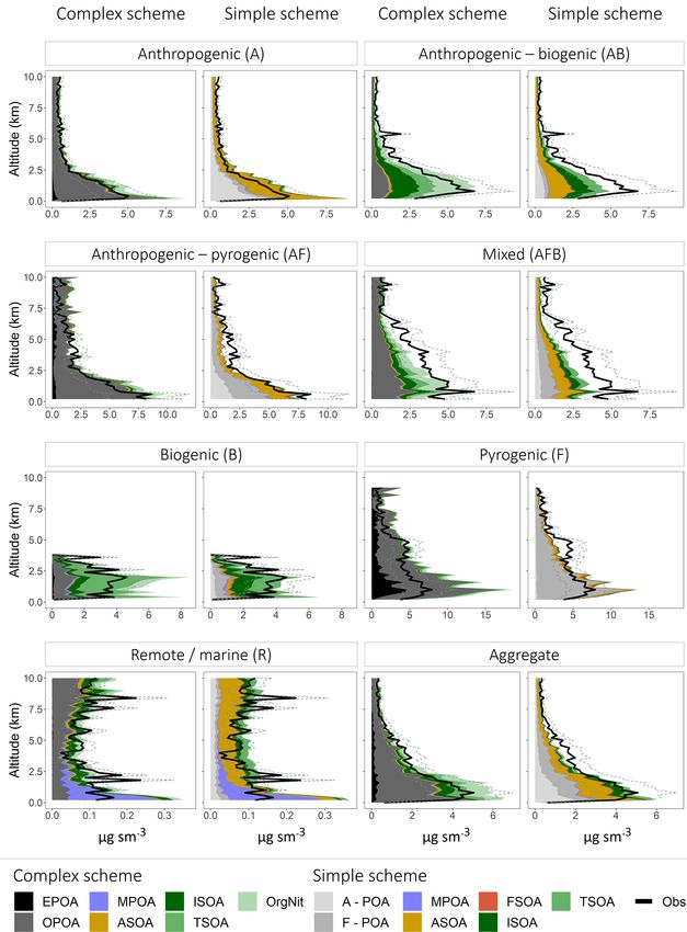
S. J. Pai et al.: An evaluation of global organic aerosol schemes using airborne observations                                        2647

Figure 5. Flight tracks colored by regime type (top). The bar plots (bottom) compare observed mean values for various species across the
different regimes. Mean values for OA are in units of micrograms per standard meter cubed (µg sm−3 ). Mean values of isoprene, nitrogen
oxides and carbon monoxide are in units of parts per billion (ppb). The regimes are as follows – anthropogenic (A), pyrogenic (F), biogenic
(B), anthropogenic + pyrogenic (AF), anthropogenic + biogenic (AB), mixed (AFB) and remote–marine (R). Refer to Sect. 3 for details on
model sampling and averaging. See Fig. S2 for altitude-differentiated maps.

tributes over 50 % of the mass are also categorized under the           averaged isoprene observations over the biogenic regime are
remote–marine regime.                                                   over 20 times greater than average measurements over the
   While we expect these model-based categories to ade-                 anthropogenic regime.
quately reflect source influences (i.e., biogenic emissions                Median concentrations over anthropogenic regions are
over the Amazon vs. anthropogenic emissions over Asia),                 markedly lower than those over other sources. Fire-
the relative mass contributions simulated by the model are              influenced regions display the highest variability, consis-
subject to large uncertainties in OA formation and lifetime.            tent with the expected source profile. Table S1 provides an
As noted in Sect. 3, sampling conditions over the regions can           overview of the observational datasets used for this valida-
vary significantly from the model treatment (such as the sam-           tion. An overview of the resulting segmentation, validation
pling of the Manaus anthropogenic plume or biomass burn-                and regime categories is provided in Table S2. Figure 5 pro-
ing plumes during the “biogenic” GoAmazon campaign).                    vides a spatial representation of the regime categorization
Due to the coarse model resolution, the regime segmenta-                for all the flight data. We note that a large proportion of the
tion described above is incapable of accurately categorizing            observations from the GoAmazon and OP3 campaigns are
some of these data points. We therefore compare the relative            densely colocated over the Amazon and Borneo and are thus
concentrations of observed NOx , CO and isoprene to inde-               difficult to discern in the figure. We also note that the “re-
pendently validate the segmentation approach. For instance,             mote” points over the southeast US represent observations in
mean observed NOx values over the anthropogenic regime                  the upper troposphere and are plotted over points in the lower
approach 1 ppb compared to 0.36 ppb over the AB regime                  troposphere, making them difficult to distinguish. Figure S2
and 0.17 ppb over the Biogenic regime, consistent with the              provides a spatial characterization of the different regimes
expected chemical signature over these regions. Similarly,              differentiated by altitude for further clarity. While the regime

www.atmos-chem-phys.net/20/2637/2020/                                                     Atmos. Chem. Phys., 20, 2637–2665, 2020
2648 S. J. Pai et al.: An evaluation of global organic aerosol schemes using airborne observations
analysis provides useful insight into the primary sources of to both sulfate and organic aerosol, such as emissions and
OA over the region, the classifications are intended to be transport, in controlling aerosol concentrations.
broad and do not, for instance, distinguish between fresh and Figure 8 shows that both the complex and simple schemes
aged aerosol contributions from the same source. For exam- exhibit substantial skill in capturing the vertical OA profile
ple, a number of points over the northern Atlantic and Pacific across the aggregate dataset, with a vertical R 2 of 0.97 and
oceans are classified as anthropogenic because they are com- 0.95 across the complex and simple schemes, respectively.
posed of a minimum of 70 % anthropogenic OA from con- Despite significant differences in the treatment of OA for-
tinental sources and are high enough in concentration to not mation and atmospheric processing (and thus the source of
be classified as “remote”. simulated OA), both schemes appear to have similar skill
in reproducing the observed vertical profile across the in-
4.3 Evaluation of model simulations against airborne dividual regimes, with the exception of the remote regime
measurements (driven largely by ATOM1-W and ATOM2-W) for which
both schemes struggle somewhat to reproduce the variabil-
Here we evaluate the two model schemes against the suite of ity in the observed vertical profile (Fig. S3). This result is
airborne observations described in Sect. 3. Despite the sub- not surprising given the low concentrations and the potential
stantial differences described in Sect. 2.1, both schemes re- for uncertainties in transport and chemical processing to be
produce the broad distribution (Fig. 6a) of OA observations. exacerbated in the remote regime. Overall, the schemes dis-
While the schemes exhibit slight offsets in their peaks near play similar skill at capturing the vertical variability across
the lower end of the distribution, there is no evidence of a the different regimes, highlighting that much of this variabil-
large systematic skew compared to observations, suggesting ity is likely driven by the prescribed transport and vertical
that there is not an obvious mode of formation or loss of mixing and is independent of the OA chemical scheme.
OA that the model fails to capture. Differences between the When compared in aggregate, the simple scheme is less
two model distributions are also relatively small, and both biased in the lower troposphere, while the complex scheme
exhibit fairly comparable skill. The simple scheme is less is less biased in the upper troposphere (Figs. 8, S3). This
biased than the complex scheme on average, with median could be due to the partitioning mechanism in the complex
OA values of 0.81 and 0.86 µg sm−3 , respectively, compared scheme that is able to model semi-volatile OPOA and SOA
to the observational median of 0.68 µg sm−3 . An analysis of with greater sophistication using the VBS framework. There
the model–observation distributions for the individual cam- are also various regime-specific differences in model perfor-
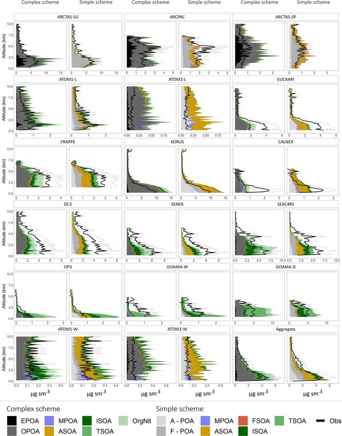
paigns (see Fig. 7) demonstrates that both model schemes mance. For instance, the complex scheme significantly over-
appear to overestimate OA mass at the low and high ends of estimates OA in the lower troposphere over fire-influenced
the distribution for several campaigns (as seen in the case of regions, likely due to the 27 % increase in primary OA
KORUS, GOAMA-W and OP3), while underestimating or- emissions to account for the dynamic partitioning between
ganic aerosol loadings in the middle of the distribution, sug- gas- and aerosol-phase POA. However, both the complex
gesting a potential mischaracterization of aerosol sources and and simple schemes underestimate OA loadings in the mid-
lifetimes over these regions. This might also be the result of troposphere over these same regions. This bias may be due
the coarse model resolution in regions with a high spatial to fire injection from large fires into the free troposphere,
variance in source strengths. Both model schemes underesti- particularly over boreal regions (Turquety et al., 2007), that
mate the lowest concentrations and overestimate the highest is not captured by the model (all emissions from fires are
concentrations over the ocean (ATOM1-W and ATOM2-W). assumed to be in the boundary layer). This shortcoming is
However, Fig. 6a suggests that these are not pervasive issues also evident over regions influenced by both anthropogenic
with the OA simulation at the global scale. We note, how- and fire emissions (AF Regime). Figure 8 also demonstrates
ever, that this could be due to an averaging effect. Figure 6b that lower-tropospheric concentrations cannot be reproduced
shows the same comparison for sulfate as a benchmark for a over oceans without the inclusion of a marine source of
species that is generally well simulated by the GEOS-Chem POA, although the comparisons suggest that the marine POA
model (Fisher et al., 2011; Heald et al., 2011; Kim et al., source may be a factor of ∼ 2 too high. While the model ap-
2015). While the comparison suggests that there continues pears to capture the vertical profile of OA in anthropogenic
to be further scope for improvement within the OA chemical regions reasonably well (Fig. 8), there are regional differ-
schemes, the model simulations are approaching the skill of ences (Fig. 9), with large model underestimates of OA in
the sulfate simulation both in terms of bias (the sulfate sim- the lower troposphere over California (CalNex), the central
ulation normalized mean bias of 0.20 is similar to the model US (DC3) and Europe (EUCAARI) as well as large overesti-
OA bias outlined above) and captured variability (with an R 2 mates over Korea and parts of the Pacific influenced by out-
of 0.62 for the model sulfate scheme relative to the obser- flow from Asia (Figs. 9, S4). These differences are consistent
vations compared to an R 2 of 0.41 and 0.44 for the simple across both the simple and complex schemes, highlighting
and complex OA schemes, respectively). This suggests the the importance of accurate anthropogenic emission inven-
potential importance of other drivers of variability common tories. The overestimate in the Asian outflow region might
Atmos. Chem. Phys., 20, 2637–2665, 2020 www.atmos-chem-phys.net/20/2637/2020/S. J. Pai et al.: An evaluation of global organic aerosol schemes using airborne observations 2649 Figure 6. (a) Distribution plots of OA mass concentrations for the complex scheme (dark green), simple scheme (light green) and AMS observations (black). The x axis has been transformed using a square-root function. Vertical lines represent median values for the different distributions. (b) Distribution plots of sulfate mass concentrations for the model (red) and AMS observations (black). Refer to Sect. 3 for details on model sampling and averaging. specifically point to the importance of constraining Asian tive bias over biogenic (B) regions (such as the Amazon), pri- IVOC emissions, given that recent studies have suggested marily driven by an overestimate in terpene SOA, potentially that SOA from IVOCs accounts for a major fraction of the to- suggesting that the scheme may not accurately capture global tal OA burden across China (Zhao et al., 2016). In regions in- biogenic SOA burdens and needs to be better constrained. fluenced by both anthropogenic and biogenic emissions (AB The overestimate of OA in both schemes in the boundary regime) the complex scheme is less biased than the simple layer over the Amazon and Borneo is accompanied by an scheme, which underestimates the observed concentrations. underestimate in the upper troposphere (Fig. 9), potentially This difference in bias is likely due to the more sophisticated indicating overly rapid model SOA formation or a failure to treatment of isoprene-derived SOA yields (through the aque- capture vertical mixing in the region. ous uptake and organic nitrate formation mechanisms) in the We note that while the observations used in this study complex scheme. The NOx -dependent yields of isoprene- have a large spatial range, they are temporally limited and and terpene-derived SOA in the complex scheme might also might not be representative of the mean state. Atypical me- be a source of increased model skill, given that organic ni- teorological conditions during the different campaigns may trates and oxidized isoprene products account for a dominant contribute significantly to the model–observation bias. For fraction of the total modeled OA in the complex scheme over example, the EUCAARI campaign was characterized by a these regions. The relative skill of the complex scheme is westward flow across Germany and the southern UK (Mor- unsurprising given that the vast majority of the AB regime gan et al., 2010), capped by a strong inversion that lim- is over the southeast US, for which the complex scheme ited vertical mixing. Similarly, differences in sampling pri- was developed and validated. However, the model skill over orities might impact the chemical composition of the obser- the AB regime may be fortuitous, given that recent studies vations in a manner that deviates from climatology. For in- have demonstrated that a significant fraction of the observed stance, the GoAmazon campaign was partially oriented to- OA over the southeast US is generated from monoterpene ward sampling anthropogenic outflow from the city of Man- precursors rather than isoprene (Xu et al., 2018; Zhang et aus (Shilling et al., 2018), impacting the OA measurements al., 2018). This potentially suggests that monoterpene SOA in a manner that the model is ill-equipped to reproduce. How- yields over the southeast US are low in the model. This may ever, despite the various gaps in model fidelity, this analysis also contribute to the underestimate of OA observed during suggests that both schemes are relatively skilled at captur- EUCAARI, which is influenced by the forests of northern ing the observed magnitude and vertical variability across Europe (Figs. 9, S4). Recent work has also demonstrated that the different regimes. A previous comparison of observed organo-nitrates contribute a significant fraction of the total vertical profiles by Heald et al. (2011) concluded that the OA mass over certain parts of Europe (Kiendler-Scharr et two-product SOA with non-volatile POA model used in ear- al., 2016), potentially indicating a model underestimate in lier versions of GEOS-Chem required additional sinks and organo-nitrate formation over the region. In contrast to its sources in order to match observations, suggesting the need skill over the US, the complex scheme displays a large posi- for photochemical sinks from photolysis and fragmentation www.atmos-chem-phys.net/20/2637/2020/ Atmos. Chem. Phys., 20, 2637–2665, 2020
You can also read