Release Guide ERDAS IMAGINE 2020 - GEOSYSTEMS
←
→
Page content transcription
If your browser does not render page correctly, please read the page content below
Release Guide

Release Guide
ERDAS IMAGINE 2020

Version 16.6
14 October 2019
Contents
About This Release ........................................................................................................................ 5

ERDAS IMAGINE Product Tiers ................................................................................................... 5

New Platforms ................................................................................................................................ 6
   Full 64-bit Installer ........................................................................................................................6
   ArcGIS 10.7 ..................................................................................................................................7
   New Licensing ..............................................................................................................................7

New Technology ............................................................................................................................. 7
   New Operators for Spatial Modeler..............................................................................................7
      Classify Buildings ......................................................................................................................7
      Extract Building Footprints ........................................................................................................8
      Compute Ground Sampling Distance .......................................................................................8
      Calculate Cell Size ....................................................................................................................8
      Grow Features ..........................................................................................................................9
      Initialize CART Regressor ......................................................................................................10
      Initialize Random Forest Regressor .......................................................................................10
      Predict Using Machine Learning.............................................................................................10
      Augment Training Data ...........................................................................................................10
      Assess Object Detection Accuracy.........................................................................................11
      Densify Geometry ...................................................................................................................11
      Smooth Geometry ...................................................................................................................11
      Arrange Items ..........................................................................................................................12
      Catch Error ..............................................................................................................................12
      Color Input ...............................................................................................................................13
      Combine ..................................................................................................................................13
      Compute GLCM Texture .........................................................................................................14
      Create Dice Boundaries..........................................................................................................16
      Create Image Pyramid ............................................................................................................18
      Delete Image Pyramid ............................................................................................................19
      Enhance Contrast Using CLAHE............................................................................................19
      Get TIFF Options ....................................................................................................................21

4 October 2019                                                                                                                                   2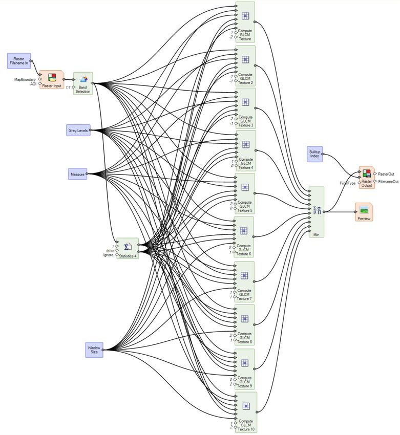
Resize Matrix...........................................................................................................................21
    Resize Table ...........................................................................................................................23
    Set Matrix Values ....................................................................................................................23
    Set Table Values .....................................................................................................................25
    Sort Items ................................................................................................................................25
    Update Image with RPCs .......................................................................................................26
 Updated Operators .....................................................................................................................26
    Classify Using Machine Learning ...........................................................................................26
    Initialize Naïve Bayes..............................................................................................................27
    Orthorectify ..............................................................................................................................27
    Set to NoData ..........................................................................................................................28
 Shared Operators .......................................................................................................................28
    Accumulate Flow .....................................................................................................................28
    Calculate Flow .........................................................................................................................29
    Fill Depressions.......................................................................................................................29
    Find Watersheds .....................................................................................................................29
    Interpolate Using IDW .............................................................................................................30
 Format Support ...........................................................................................................................30
    Cloud Optimized GeoTIFF ......................................................................................................30
    MIE4NITF ................................................................................................................................31
    GeoPackage............................................................................................................................32
    Luciad Terrain Service ............................................................................................................33
    NetCDF....................................................................................................................................33
    WMS display optimizations .....................................................................................................33
 General ERDAS IMAGINE .........................................................................................................34
    Image Chain Printing ..............................................................................................................34
    Optimal Seamline Generation.................................................................................................34
    3Dconnexion SpaceMouse Pro ..............................................................................................34
    Copy Selected Breaklines.......................................................................................................35
    Editing Breakline Vertices .......................................................................................................35
    Dynamic update of Contours during Breakline editing...........................................................36
    Consistent Style Library locations ..........................................................................................36

4 October 2019                                                                                                                                 3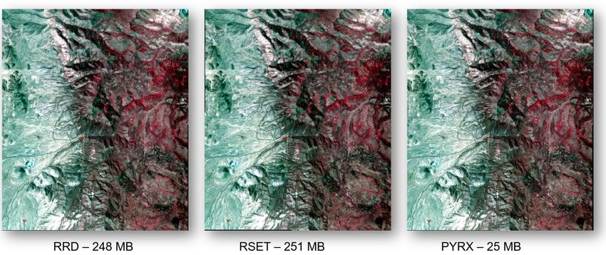
System Requirements ................................................................................................................. 37
   ERDAS IMAGINE .......................................................................................................................37
   ERDAS IMAGINE System Requirements Notes .......................................................................38

Issues Resolved ........................................................................................................................... 39
   IMAGINE Essentials ...................................................................................................................39
   IMAGINE Advantage ..................................................................................................................57
   IMAGINE Objective ....................................................................................................................59
   IMAGINE Photogrammetry.........................................................................................................59
   IMAGINE Professional................................................................................................................63
   IMAGINE SAR Interferometry ....................................................................................................66
   Spatial Modeler ...........................................................................................................................66
   IMAGINE Terrain Editor .............................................................................................................78
   IMAGINE Expansion Pack – 3D.................................................................................................78
   IMAGINE Expansion Pack – AutoSync......................................................................................79
   IMAGINE Expansion Pack – NITF .............................................................................................80
   ERDAS IMAGINE Installation ....................................................................................................81
   ERDAS ER Mapper ....................................................................................................................81
   PRO600 ......................................................................................................................................82
   Stereo Analyst for ERDAS IMAGINE .........................................................................................83

Contact Us .................................................................................................................................... 85
About Hexagon ............................................................................................................................. 85
Copyright.......................................................................................................................................86

4 October 2019                                                                                                                                  4
About This Release
This document describes the enhancements for ERDAS IMAGINE 2020 (v16.6.0), including IMAGINE
Photogrammetry (formerly LPS Core) and ERDAS ER Mapper. Although the information in this document is
current as of the product release, see the Hexagon Geospatial Support website for the most current version.

This release includes both enhancements and fixes. For information on fixes that were made to ERDAS
IMAGINE for this release, see the Issues Resolved section.

This document is only an overview and does not provide all the details about the product's capabilities. See
the online help and other documents provided with ERDAS IMAGINE for more information.

Development of ERDAS IMAGINE 2020 focussed on ensuring that virtually all aspects of ERDAS IMAGINE
run in 64-bit. Consequently, the installer has been split into three separate installers: ERDAS IMAGINE 2020
64-bit; ERDAS IMAGINE 2020 32-bit; and ERDAS ER Mapper 2020.

In addition, there are new Operators, such as the Compute Grey-Level Co-Occurrence Matrix operator, as well
as numerous software quality improvements.

ERDAS IMAGINE Product Tiers
ERDAS IMAGINE® performs advanced remote sensing analysis and spatial modeling to create new
information. In addition, with ERDAS IMAGINE, you can visualize your results in 2D, 3D, movies, and on
cartographic-quality map compositions. The core of the ERDAS IMAGINE product suite is engineered to scale
with your geospatial data production needs. Optional modules (add-ons) providing specialized functionalities
are also available to enhance your productivity and capabilities.

IMAGINE Essentials® is the entry-level image processing product for map creation and simple feature
collection tools. IMAGINE Essentials enables serial batch processing.

IMAGINE Advantage® enables advanced spectral processing, image registration, mosaicking and image
analysis, and change detection capabilities. IMAGINE Advantage enables parallel batch processing for
accelerated output.

IMAGINE Professional® includes a production toolset for advanced spectral, hyperspectral, and radar
processing, and spatial modeling. Includes ERDAS ER Mapper.

IMAGINE Photogrammetry maximizes productivity with state-of-the-art photogrammetric satellite and aerial
image processing algorithms.

4 October 2019                                                                                                 5
New Platforms
Full 64-bit Installer
On modern 64-bit computers, being able to run as a true 64-bit application allows full exploitation of the
computer’s resources, including addressing more than 4GB of memory.

Over the previous few releases Hexagon has been moving more and more ERDAS IMAGINE executables to
run 64-bit. With each such release a few non-GUI applications (jobs) were made available in both 32-bit and
64-bit and the user was able to configure which one was run by the Session Manager. In ERDAS IMAGINE
2018 we released the main Ribbon GUI (ewkspace.exe) in both 32-bit and 64-bit, but whether applications
launched from either of these configurations ran as 32-bit or 64-bit (if available) was still variable, depending
on the 64-bit configuration settings. This mixed approach presented some problems, not least the lack of
transparency to the user as to whether the job they were about to execute would run 32-bit or 64-bit.

Consequently, ERDAS IMAGINE 2020 has been clearly split into two separate installers (plus a third one for
ERDAS ER Mapper): One in which the entire suite runs as 32-bit applications and one in which the entire suite
runs as 64-bit. This means that if someone starts ERDAS IMAGINE 2020 64-bit they can be sure that any
feature they utilize will be running 64-bit and is therefore capable of exploiting larger amounts of system
memory and other resources.

This split also makes any configuration tasks much more straightforward. If you want to use Python with
ERDAS IMAGINE 2020 32-bit, then you need a 32-bit version of Python. If you want to configure CSM/MSP to
work with ERDAS IMAGINE 2020 64-bit, then you just need 64-bit CSM/MSP, etc.

Note that all three installers (ERDAS IMAGINE 2020 64-bit, ERDAS IMAGINE 2020 32-bit, and ERDAS ER
Mapper 2020) can be installed on a single computer if needed.

If 64-bit is so great, why do we still have ERDAS IMAGINE 2020 32-bit? Unfortunately, not every program
could be ported to 64-bit, usually because there was a dependency on a third-party component that is only
made available in 32-bit. These occurrences are very limited compared to the number of programs that have
been successfully included into ERDAS IMAGINE 2020 64-bit. However, there is a possibility that a production
workflow is depending on one of these capabilities and so ERDAS IMAGINE 2020 32-bit is being provided so
that customers who need these capabilities can continue to use them if needed.

The functionality that is only available in ERDAS IMAGINE 2020 32-bit is as follows:

    •   Image Equalizer
    •   Image Catalog
    •   StereoSAR DEM
    •   IMAGIZER
    •   External Projections
    •   Surfacing Tool (deprecated in favour of Terrain Prep tool)
    •   ESRI Grid support
    •   MultiGen OpenFlight format support
    •   Oracle Geospatial Raster support
    •   ArcSDE support
    •   TerraModel TIN support
    •   IRS Sensor Model
    •   MapInfo support
    •   Geodatabase support

Depending on component availability, some of these capabilities may find their way back into a 64-bit version
of ERDAS IMAGINE in the future.

4 October 2019                                                                                                      6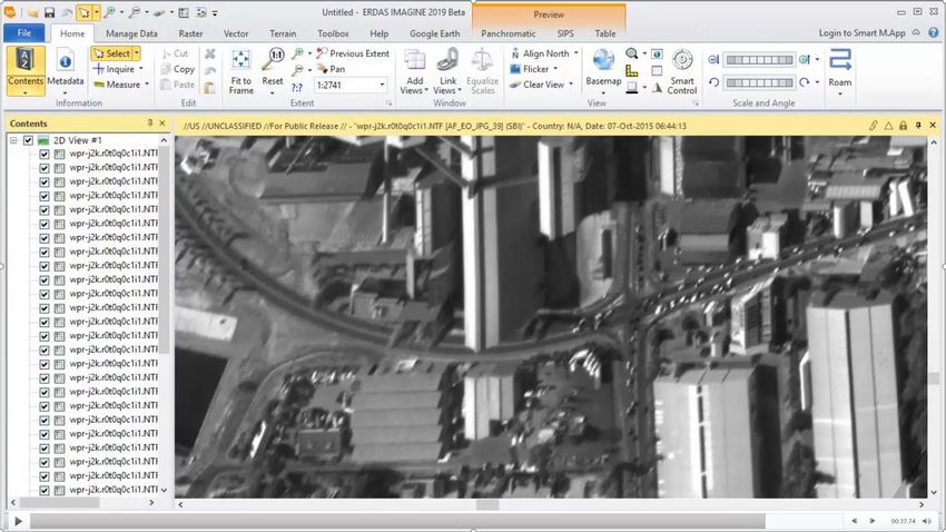
ArcGIS 10.7
ERDAS IMAGINE 2020 (32-bit) has been tested and declared Supported when using an installed and licensed
version of ArcGIS 10.6, 10.6.1 and 10.7 in order to provide Geodatabase support libraries.

Alternatively, the IMAGINE Geodatabase Support component (based on ArcGIS Engine 10.7) can be installed
to provide Geodatabase support.

Please note that at this time ArcGIS 10.7.1 is not supported.

New Licensing
ERDAS IMAGINE 2020 is delivered with version 16.6.9.110 of the Hexagon Geospatial Licensing 2020 tools.
However, if there is a newer version available for download it is strongly recommended that customers
upgrade to the newer version. The appropriate download can be found on the Downloads section of the
Hexagon Geospatial web site:

https://download.hexagongeospatial.com/search?lang=en&product=b3b4786d3d4742ae8d1e7aeee50dae69

Since Hexagon Geospatial Licensing 2020 v16.6.9.110 is integrated into the ERDAS IMAGINE 2020 installer,
any computer where you install will have any existing installation of Hexagon Geospatial Licensing
automatically updated to v16.6.9.110. If in doubt, refer to Windows’ Add or Remove Programs utility to
determine the currently installed version.

New Technology
New Operators for Spatial Modeler
Hexagon has continued to add new operators to Spatial Modeler. New (or modified) operators with a brief
description of their capabilities are described below. See the ERDAS IMAGINE 2020 Help for full details of
each operator, as well as the Hexagon Geospatial Community > Spatial Recipes page, for examples of Spatial
Models that use many of these capabilities.

Classify Buildings

The operator identifies points from the input point cloud that fall on buildings and reassigns them to the
Building class (Class 6). The operator requires that the points that fall on the ground in the point cloud have
already been classified, that is, assigned to the Ground class (Class 2). If the ground points in the input point
cloud are not classified, you can classify them using the Classify Ground operator.

The classification is performed by analyzing the geometric relationship of the non-ground points to their
neighbors, looking for planar areas above ground that satisfy the specified height and area criteria.

4 October 2019                                                                                                      7
Extract Building Footprints

The operator extracts building footprints based on points in the point cloud that have already been classified
as Building points (Class 6). The operator requires that the points in the point cloud that fall on the ground and
on buildings have already been classified to the Ground class (Class 2) and the Building class (Class 6)
respectively.

Compute Ground Sampling Distance

This operator computes the ground sampling distance for a point cloud by analysing the distance between
adjacent points. By default, the first 1000 points having last and single returns are included in the computation.
You may override this by putting data on the SelectionCriteria port. Typically, the output from this operator is
used to specify the cell size when converting from point cloud to raster.

Calculate Cell Size

This operator calculates appropriate ground-space pixel dimensions for an input grid or image that is to be
resampled. This is most frequently required if the input grid is a referenceable grid to be orthorectified (such as
a NITF image with embedded RPCs), or if the input grid is to be reprojected to a different CRS.

The algorithm used has also been integrated into standard ERDAS IMAGINE resample dialogs so that the
default pixel size populated into the dialogs should attempt to retain the optimal level of precision (without
over-sampling).

4 October 2019                                                                                                   8
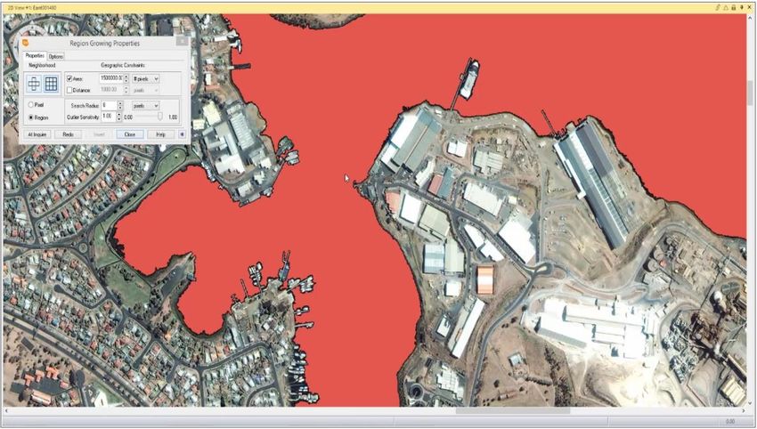
Grow Features

Grow features operator extracts features from raster data and seed pixel(s) by growing the seed pixel(s) into
larger regions. Regions are grown by adding neighbouring pixels that are spectrally similar to the seed
pixel(s). Each neighbour pixel is evaluated to measure if it is spectrally similar to the seed and, if it is, it is
incorporated into the region. The enlarged region then has new neighbours to be evaluated. This process
continues until no new neighbours are added to the region being grown (or one of the other growing
constraints is met).

The improved region growing algorithm has also been integrated into the 2D Views vector editing tools:

4 October 2019                                                                                                        9
Initialize CART Regressor

This operator defines and trains a CART regressor that is used as an input for estimating data using the
Regression Using Machine Learning operator.

Initialize Random Forest Regressor

This operator defines and trains a Random Forest regressor that is used as an input for estimating data using
the Regression Using Machine Learning operator.

Predict Using Machine Learning

This operator performs regression on the input data using the trained regressor specified on the
MachineIntellect port. The input data can be of type IMAGINE.Features or IMAGINE.Raster.

Augment Training Data

4 October 2019                                                                                             10
This operator creates additional training data for Classify Using Deep Learning by modifying existing training
data. Depending on the selected options, it will produce rotated, scaled, translated and flipped versions of the
input training data.

Assess Object Detection Accuracy

Object detection accuracy assessment is a process in which the result from object detection is compared to
ground truth data to measure the agreement between the two. This operator performs accuracy assessment
by comparing the rectangular bounding box and class attribute of the objects that represent the ground truth
with the objects detected from the object detection.

Densify Geometry

Densify Geometry operator adds vertices to the geometry of the input features using a maximum distance
factor. If the distance between two vertices is larger than MaxDistance, a new vertex is inserted halfway
between the two vertices. This repeats until no segment between vertices is larger than MaxDistance, or until
the output geometry exceeds the size of MaxSize.

Smooth Geometry

Smooth Geometry operator smooths the geometry of the input features using a weighted-average smoothing
algorithm. Smoothing shifts the position of points on a geometry in order to remove small perturbations and
capture only the most significant trends. Unlike simplification, smoothing preserves the number of points in a
geometry but improves their appearance. The operator offers control over the algorithm through a
densification tolerance, look-ahead count, and weighting factor.

4 October 2019                                                                                                11
Arrange Items

Selects, arranges, and duplicates values from a list or table given the order specified on the RangeList port, to
create an output list or table.

Examples:

Given DataIn [ -2 , 0 , 2 , 3 , 7 , 8 ] and RangeList [ 0 , 1 , 3 , 0 , 3 , 5 ], DataOut results in [ -2 , 0 , 3 , -2 , 3 , 8 ]

Given DataIn [ -2 , 0 , 2 , 3 , 7 , 8 ] and RangeList [ 0:2 , 1:4 ], DataOut results in [ -2 , 0 , 2 , 0 , 2 , 3 , 7 ]

This operator is often used in conjunction with the output created by the Sort Items operator so that a set of
values can be ordered in the same manner as another set of values. For example, consider two Tables, one
consisting of Class Names and another consisting of the Histogram values associated with those Class
Names. If the Class Names Table is sorted alphanumerically, the Table of Histogram values could be re-
organized so that the Histogram values are still ordered correctly against their corresponding Class Names by
using the Indices output by Sort Items as the RangeList input to this operator.

Catch Error

This operator transforms the condition of whether an error occurs in the execution of the contained submodel
into a boolean result.

This operator can be useful, for example, in allowing an iterative submodel to execute to completion over a
collection of dataset references of uncertain applicability. If the submodel illustrated below were placed into an
Iterator fed by a Multi Filename Input operator result, any file names that were not appropriate for the Raster
Input operator contained in the Catch Error submodel would end up in the BadFilenameOut list.

4 October 2019                                                                                                             12
Contents of an Iterator operator using Catch Error:

Catch Error submodel:

Color Input

Creates a Color. Double-click the operator to open its configuration dialog. The Color Chooser opens. The
Color to be output is placed on the Input port, which is hidden by default.

Combine

Combines multiple lists into a single list. A new List/Table is created consisting of each element of the
Lists/Tables provided, in the order provided (Collection1's element will be followed by Collection2's element,
etc.). This is an expandable operator, so you can add as many Collection ports as required.

The model below shows how to Combine two Tables together.

4 October 2019                                                                                              13
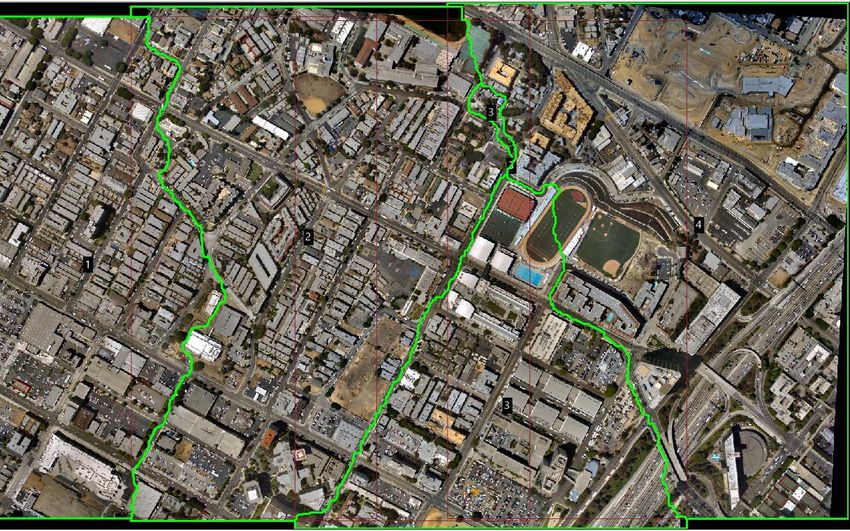
Compute GLCM Texture

Computes a texture feature for an input image. The specified texture feature is computed from various
statistical properties of a per-pixel internally generated gray-level co-occurrence matrix (GLCM).

Texture Computations using a Grey-Level Co-Occurrence Matrix are usually considered to be "second order"
measures of texture present in the original image. Traditional texture measures are usually considered "first
order" since the texture measures are statistics calculated from the original image values, like variance, and
do not consider pixel neighbor relationships. Conversely "second order" measures consider the relationship
between groups of two (usually neighboring) pixels in the original image.

Such texture measures are considered highly useful as derived information for input into other processes such
as image classification, especially Machine Learning, and other purposes, such as to identify built-up areas in
the example below:

4 October 2019                                                                                              14
Note that GLCM calculations are highly compute intensive and so benefit from the presence of a GPU-enabled
graphics card running OpenCL.

4 October 2019                                                                                         15
Create Dice Boundaries

Create Dice Boundaries splits up the boundary of an image into smaller, regularly sized and spaced
boundaries that can be used for subsetting. Neighboring new boundaries can overlap each other by an extent
specified by the XOverlap and YOverlap ports.

The example Spatial Model shown below uses the Create Dice Boundaries operator to create a regular grid of
area polygon geometries over an image, which could then be used for Zonal Change Detection or Deep
Learning feature extraction.

4 October 2019                                                                                          16
4 October 2019 17
Create Image Pyramid

This operator ensures the existence of an image pyramid and statistics for an image dataset.

It produces or verifies the existence of a persistent, optimal sequence of images, each of which is
progressively lower in resolution than the preceding image in the sequence. The primary use of an image
pyramid is to increase rendering speed and reduce aliasing artifacts when visualizing the image at scales
larger than its original resolution.

If you want to ensure that all image pyramids are of the type (Generator) and are created using the
downsampling method specified or you want to force new image pyramids to be created, use the Delete
Image Pyramid operator ahead of this operator.

It also ensures that image statistics are available for the image. This occurs even if a suitable image pyramid
is already present.

One major advantage of this new mode of generating pyramid levels is the ability to create PYRX format
pyramid files. These use ECW compression and consequently are not only fast but also take up far less disk
space than traditional pyramid file formats.

In the example below, the original satellite image was 713MB in size. Three different formats of pyramid file
were generated and the image displayed Fit to Frame. The PYRX pyramid file is 1/10th the size of the other
two formats while maintaining display quality.

Please note that Create Image Pyramid replaces all the functionality formerly provided by Create RSETs.
Create RSETs should no longer be used.

4 October 2019                                                                                                  18
The new modes of generating pyramid files have also been built into the Raster Output operator, Image
Commands tool (Home tab > Information group > Metadata pulldown > Edit Image Metadata) for batch
creation of pyramids, the Image Metadata dialog (Home tab > Information group > Metadata pulldown >
View/Edit Image Metadata), as well as any application that uses Spatial Modeler for performing its processing.
The type of Generator used by default, as well as the associated downsampling technique, can be controlled
via Preferences.
Note: if routinely running ERDAS IMAGINE 2020 32-bit (as opposed to the 64-bit version) you may encounter
errors regarding insufficient memory when processes attempt to create .pyrx formatted pyramid files for larger
image files. If this occurs there are two possible workarounds (other than running ERDAS IMAGINE 2020 64-
bit):
• In the Preference Editor (File > Preferences) reduce the amount of memory allowed for the Spatial
Modeler to run by changing Percentage of Available Memory to Consume to a lower value (such as
30%). This allows the ECW/JP2 Encoding engine more memory to perform the compression
• Or, alter the Pyramid Layer Generator preference from the default setting to “Always use the RRD
Pyramid Generator”. This effectively sets the software to produce pyramid files in the manner it did
prior to the 2020 release.
Delete Image Pyramid
Delete Image Pyramid deletes existing image pyramid from a raster image.
All image pyramids that are discovered will be deleted (if possible). This includes:
• ERDAS Reduced Resolution Dataset (*.rrd)
• Extended compressed image pyramid (*.pyrx)
• NITF RSET
• Minifiles
• GDAL Overviews (*.ovr)
Pyramids that cannot be deleted include:
• Pyramids internal to IMAGINE Image (*.img)
• Pyramids from Wavelet Compression (*.ecw, *.jp2, *.sid)
Enhance Contrast Using CLAHE
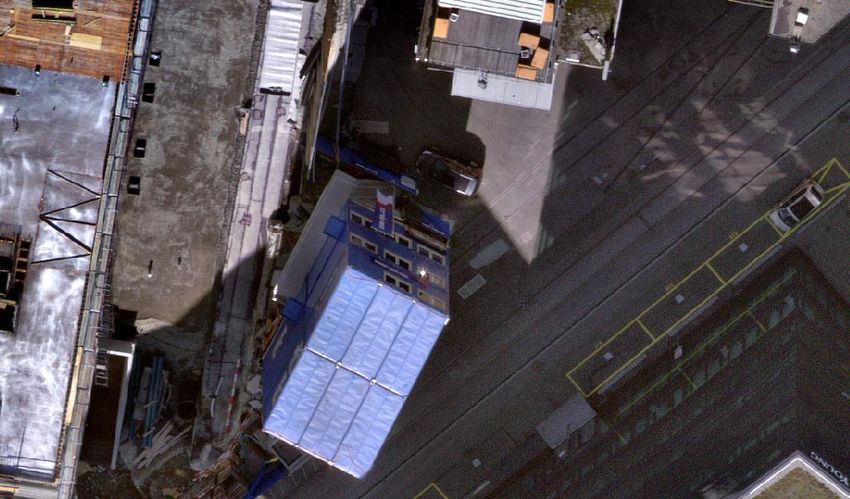
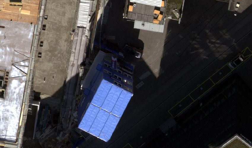
4 October 2019 19Contrast Limited Adaptive Histogram Equalization (CLAHE) algorithm is a technique used to enhance contrast in images. Traditional Histogram Equalization uses a single transformation derived from the image histogram to transform all pixels. As such it is difficult to derive a single transformation that can balance the contrast in dark, light and mid-tone areas of the histogram, especially when the data being displayed has a dynamic range larger than 8-bit (and the rendering software or display device only supports 8-bits per color channel). So techniques such as CLAHE were developed to spatially adapt the transformation and reveal the detail in dark and bright areas of a raster while maintaining contrast in mid-tone areas. For example, CLAHE can enhance hidden detail in the shadows cast by large buildings, clouds, etc. In these locations the pixel DN values will be low, but for sensors with 10, 11, 12-bit or greater dynamic ranges there may still be a wide range of values present, but the global look-up table used to render the image to an 8-bit per color channel display bins all those shadow areas into a few dark bins (i.e., low visual contrast). The spatially adaptive nature of CLAHE allows the inherent contrast in these shadow areas to be broadened and brightened to balance with neighboring non-shadow areas. For example, here’s a 12-bit color image with both bright areas and dark shadows that with a standard LUT shows little detail in the shadows: The screenshot below shows the result of using the Enhance Contrast Using CLAHE operator with a Contrast Retention Factor of 0.2: 4 October 2019 20
As can be seen, contrast is enhanced in the shadow areas without saturating the already bright areas.

Get TIFF Options

Creates the format specific output option dictionary for Tagged Image File Format (TIFF), which can then be
fed to the Raster Output operator to control format-specific output parameters, such as wanting BigTIFF
format, an alpha channel persisted, data compression, etc.

Resize Matrix

4 October 2019                                                                                            21
The purpose of this operator is to take an existing Matrix and alter the dimensions of that Matrix by either
removing rows and/or columns or adding new rows and/or columns (or any combination thereof). If adding
new rows and/or columns, the values to be used in those new cells can be specified. If removing rows, they
are removed from the bottom of MatrixIn, and if removing columns, they are removed from the right side of
MatrixIn. Similarly, if adding rows, they are added to the bottom of MatrixIn, and if adding columns, they are
added the right side of MatrixIn.

If extending MatrixIn in one dimension only (either rows or columns), you may supply a Matrix for
InitialValues. If extending the number of rows, the Matrix provided for InitialValues must have the same
number of columns as MatrixIn. It may have either a single row or as many rows as are being added to the
Matrix. If it contains a single row, all rows being added to the Matrix are filled with the single row. If extending
the number of columns, the Matrix provided for InitialValues must have the same number of rows as
MatrixIn. It may have either a single column or as many columns as are being added to the Matrix. If it
contains a single column, all columns being added to the Matrix are filled with the single column.

Examples using a MatrixIn with five rows and nine columns:

    •   Setting NumRows of 8 and NumColumns of 14 will extend the Matrix by three rows and five columns and set
        the new cells to InitialValues, which must be a Scalar. If InitialValues is -1, MatrixOut would be

    •   If InitialValues is a Matrix with one row and nine columns,

        column 0 of the added rows will be set to the value in cell 0,0 in the InitialValues Matrix, column 1 of the added
        rows will be set to the value in cell 0,1 in the InitialValues Matrix, etc. MatrixOut would be

4 October 2019                                                                                                           22
• If InitialValues is a Matrix with three rows and nine columns,
the first added row will be set to the values in row 0 of the InitialValues Matrix, the second added row will be set
to the values in row 1 of the InitialValues Matrix, and the third added row will be set to the values in row 2 of the
InitialValues Matrix. MatrixOut would be
Resize Table
Adjusts the number of rows in a Table (up or down). The InitialValues port takes a Table as input and so this
operator can be used to append Tables together.
Set Matrix Values
The purpose of this operator is to take an existing Matrix and modify specific cells of that Matrix with user-
specified values.
If only RowRangeList or ColumnRangeList is provided (the cells in all columns of one or more rows or all
rows of one or more columns are being set), you may supply a Matrix for Values. If only RowRangeList is
provided, the Matrix provided for Values must have the same number of columns as MatrixIn. It may have
either a single row or as many rows as are specified in RowRangeList. If it contains a single row, all rows
specified in RowRangeList will be filled with the single row. If only ColumnRangeList is provided, the Matrix
provided for Values must have the same number of rows as MatrixIn. It may have either a single column or
4 October 2019 23as many columns as are specified in ColumnRangeList. If it contains a single column, all columns in
ColumnRangeList will be filled with the single column.
Note that both RowRangeList and ColumnRangeList are 0-based indices. I.e. the first row is row 0, the
second row is row 1, etc.
Examples using a MatrixIn with five rows and nine columns:
• Setting a RowRangeList of 1:1,3:4 (three rows) and ColumnRangeList of 2:4 (three columns), will set the cells
at 1,2, 3,3, and 4,4 to Values, which must be a Scalar. If Values is -1, MatrixOut would be
• RowRangeList of 2:4 with no ColumnRangeList will set all cells in rows 2, 3, and 4 to Values. Values may be
either a Scalar, a Matrix with one row and nine columns, or a Matrix with three rows and nine columns.
If Values is a Scalar, all cells in rows 2, 3, and 4 will be set to that value. If Values is -1, MatrixOut would be
• If Values is a Matrix with one row and nine columns,
column 0 of rows 2, 3, and 4 will be set to the value in cell 0,0 in the Values Matrix, column 1 of rows 2, 3, and 4
will be set to the value in cell 0,1 in the Values Matrix, etc. MatrixOut would be
4 October 2019 24• If Values is a Matrix with three rows and nine columns,
row 2 will be set to the values in row 0 of the Values Matrix, row 3 will be set to the values in row 1 of the Values
Matrix, and row 4 will be set to the values in row 2 of the Values Matrix. MatrixOut would be
Set Table Values
Set Table Values sets the values of specified rows in a Table.
If the same row number is specified multiple times in RangeList, the value of that row in the Table will be set
each time. That means that if Values is a Table, the value of that row in TableOut will be what it was set to
the last time that row was specified in RangeList. For example, if TableIn is [83,208,180,96,45,234],
RangeList is [1:3,1:1] and Values is [34,27,160,69], TableOut will be [83,69,27,160,45,234].
Sort Items
Takes a List or Table and creates a List or Table of values and a List of indices (0-based), which are sorted via
the specified Order (Ascending/Descending).
For example:
• Ascending order. Given DataIn [ 15,12,17,13 ], DataOut is [ 12,13,15,17 ] and Indices is [ 1,3,0,2 ]
• Descending order. Given DataIn [ 15,12,17,13 ], DataOut is [ 17,15,13,12 ] and Indices is [ 2,0,3,1 ].
The output Indices are used in conjunction with the Arrange Items operator so that a set of values can be
ordered in the same manner as another set of values. For example, consider two Tables, one consisting of
Class Names and another consisting of the Histogram values associated with those Class Names. If the Class
Names Table is sorted alphanumerically, the Table of Histogram values could be re-organized so that the
4 October 2019 25Histogram values are still ordered correctly against their corresponding Class Names by using the Indices output by this operator as the RangeList input to the Arrange Items operator. Update Image with RPCs Some image format readers do not automatically recognize the associated Rational Polynomial Coefficient (RPC) information. In this case, the user must manually geometrically calibrate (update) the RPC information to the image so that ERDAS IMAGINE can use that information to accurately georeference the data. This operator uses the RasterFilename and SensorModelName to locate and use an RPC file to update the image. The optional RPCFilename is offered as an input in case the operator fails to automatically locate the file. Updated Operators Classify Using Machine Learning A new output port called TrainingAttributeImportances has been added. When the operator is run, this port produces a dictionary containing the names of the attributes used for classification and their associated importance to the classification. These values range from 0 to 1 and the summed importance of all training attributes is defined to be 1. If MachineIntellect does not support this output measure, all importances are equal to 1/. The importance values can be extremely useful in identifying the most important input variables contributing to successful classifications (and perhaps more importantly in identifying the unimportant variables so they can be excluded from later classifications, making the classification process more efficient). 4 October 2019 26
Initialize Naïve Bayes

This operator defines and trains a Naive Bayes classifier that is used as an input for classifying data using the
Classify Using Machine Learning operator.

A new input port called TrainingAttributesScaling can be used to scale the training attribute values to a similar
range. Scaling may improve training speed and classification accuracy.

Orthorectify

Data in a raster stream may be georeferenceable rather than being georectified (in older parlance, the data is
geometrically calibrated with a 2D or 3D geometric model as opposed to being rectified to a projected
coordinate system). Under normal circumstances, Spatial Modeler will maintain the georeferenceable state,
but some workflows might require that a georeferenceable raster be persisted in its georectified state. The
Orthorectify operator fulfils this role.

In ERDAS IMAGINE 2020 the Orthorectify operator has been updated with a number of new ports in order to
combine functionality that previously required use of a Warp operator.

    •   CellCalculationMethod
    •   AllowApproximation
    •   ApproximationTolerance
    •   ApproximationMaxOrder
    •   ApproximationGridSize
    •   UsePyramids

4 October 2019                                                                                                 27
Set to NoData The input NoDataValue port now accepts a Raster as input. This is useful for using one raster layer to mask another. If the input to NoDataValue is Scalar, the input raster stream is filtered so that every pixel value that matches the value specified on the NoDataValue port is marked as NoData in the output raster stream. If the input to NoDataValue is Raster, pixel locations in that raster that are marked as NoData are marked as NoData in the output raster stream. Note that areas outside the raster extent of the NoDataValue raster are considered NoData. Any pixels in the input raster stream that were already marked as NoData remain marked as NoData. The original value of pixels marked as NoData is not maintained. Shared Operators The following operators are licensed for use by licensed users of IMAGINE Advantage, IMAGINE Professional, GeoMedia Advantage, and GeoMedia Professional. Spatial Models using these operators will not be executable using IMAGINE Essentials or GeoMedia Essentials. Accumulate Flow The Accumulate Flow operator is part of a collection of grid operators used for hydrological analysis. It takes a FlowRaster and computes the flow accumulation for the entire surface. The AccumulationRaster produced by the Accumulate Flow operator contains data where each pixel value indicates the total number of pixels that contribute to the flow into that pixel. Pixels with a value of zero indicate headwater pixels (pixels that have no inflow, only outflow). Pixels with a value of NoData indicate no flow. The AccumulationRaster can be used as part of hydrological analysis workflows to identify river/stream networks or to identify drainage outlets, which can be used to find watershed (drainage basin) areas. 4 October 2019 28
Calculate Flow

Calculate Flow operator is part of a sequence of operators to identify drainage networks and watersheds.

Calculate Flow operates on a Raster of continuous surface elevation data, such as a Digital Elevation Model
(DEM). It generates a FlowRaster where each pixel value represents the direction that runoff would flow (in
effect, the steepest slope) over the terrain.

For each pixel, the slope of the line segment connecting the center of the pixel with the centers of the eight
adjacent pixels is computed, taking both horizontal and vertical distance into consideration. The horizontal
distance between the pixel center and the centers of the four directly adjacent pixels is equal to the pixel
resolution. The horizontal distance between the pixel center and the centers of the four diagonally adjacent
pixels is equal to the square root of two times the pixel resolution.

Runoff is assumed to flow in the direction of the steepest downhill slope. "Ties" are allowed, that is, runoff can
flow in more than one direction. Result pixel values indicate flow direction.

For the purpose of hydrological analysis, one should first run the Fill Depressions operator on the DEMRaster
to create a depression-less surface. This depression-less surface when used as the input DEMRaster to the
Calculate Flow operator will produce a FlowRaster with no ambiguous flow. This new FlowRaster can then be
used as input to the Accumulation Flow operator.

Fill Depressions

Fill Depressions operator is part of a collection of raster operators for hydrological analysis. It can be used as
part of a sequence of raster operators to identify drainage networks and watersheds.

Fill Depressions operates on a Raster of continuous surface elevation data, such as a Digital Elevation Model
(DEM). It generates a FilledRaster where minor depressions in the surface have been removed.

Find Watersheds

In hydrological analysis, a watershed, or drainage basin, is defined as an area of land where all water (rainfall,
streams, rivers, etc.) drains to a common outlet. Watersheds can be small, as in the area of land that drains

4 October 2019                                                                                                   29
into a single reservoir or into a single stream segment, or large, as in the area of land that drains into the
mouth of a major river. The Find Watersheds operator is part of a collection of raster operators used for
hydrological analysis. It uses a FlowRaster to find the watershed areas where water drains to common flow
outlets identified by the OutletRaster.
FlowRaster must contain data that indicates the downhill drainage flow direction for each cell.
OutletRaster contains data that uniquely identifies the common flow outlets for which watershed areas are to
be found. The pixels that define a common flow outlet for a watershed should be assigned the same integer
value. OutletRaster can define common flow outlets for multiple watersheds and each should be assigned a
unique integer value. All pixels that do not define watershed flow outlets must be assigned to NoData.
OutletRaster can define common flow outlets as a single or small set of pixels at the mouth of a stream or
river, as a linear set of pixels defining a stream network or stream segments, or as clumps of pixels defining
ambiguous flow zones.
WatershedRaster produced by the Find Watersheds operator contains data showing the watershed areas
found for each uniquely identified common flow outlet defined in the OutletRaster. The pixels that define a
watershed area are assigned the same integer value as its associated common flow outlet pixels. All pixels
that are not assigned to a watershed are set to NoData.
Interpolate Using IDW
Interpolate Using IDW performs an interpolation function that uses an Inverse Distance Weighting (IDW)
algorithm to attempt to create a continuous raster data set from data that is incomplete. It computes values for
NoData locations based on neighboring pixels with values.
The operation works best with semi-continuous data such as contours or remote sensing imagery with gaps.
For very sparse point data such as spot heights, geological surveys, clustered data, and random points, apply
a kriging process to interpolate a continuous data set. Interpolate Using IDW should be used when processing
the following scenarios:
• For height density and/or regular spaced data points, such as elevation data, temperature data, rainfall data, or
data from any continuously varying surface.
• To fill in small gaps in satellite data, airphoto mosaics, or Digital Elevation Model (DEM) mosaics.
• When there is a low degree of confidence in the exactness of the original data.
• To create a DEM from contour or ridge-and-channel data.
Format Support
Cloud Optimized GeoTIFF
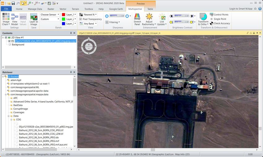
ERDAS IMAGINE 2020 enables access to public and private Amazon S3 cloud storage services via the
Retriever pane. One of the most effective formats to use via these services is the Cloud Optimized GeoTIFF
(COG) format.
Data accessed in this manner can be used in Spatial Model Editor or displayed via Image Chain.
4 October 2019 30MIE4NITF Time-series datasets are now being stored and delivered in the MIE4NITF standard. This can consist of hundreds, even thousands, of individual image frames stored in a NITF. ERDAS IMAGINE 2020 has been enhanced to enable opening multiple MIE4NITF frames into tools such as the Flicker tool in order to “play” the time-series, as well as being able to open individual frames for further exploitation. 4 October 2019 31
GeoPackage
Spatial Modeler and the Image Chain are capable of reading raster data stored in the popular GeoPackage
format. Vector features can also be accessed through the Spatial Modeler.

4 October 2019                                                                                            32
Luciad Terrain Service
Luciad Terrain Services from LuciadFusion can be consumed in ERDAS IMAGINE as standard raster data
sources, enabling their use for orthocorrection and other purposes.

NetCDF
Spatial Modeler and the Image Chain are capable of reading raster data in the NetCDF format.

WMS display optimizations
ERDAS IMAGINE’s 2D View works largely on the basis of pulling tiles from the source data for display. These
tile requests (which cover an extent larger than the extent of the 2D View) appear to be causing WMS servers
problems when they are expecting to return just one tile covering the entire desired extent.

Consequently, for ERDAS IMAGINE 2020 we have introduced a second display mode/option for use with all
WMS data layer types. This option is presented as a checkbox button in the Ribbon interface called
"Continuous Roaming" and defaults to Off (that is, the new behavior).

Turning this checkbox on will result in requests to the WMS server being for tiles rather than for the View
extent. The benefit of turning the mode on is that tile requests can be sent and data rendered to screen while
the extent is being panned or zoomed (for example, while the middle mouse button is still held down and the
data being dragged). The downside is that the overall time to fill a View extent may be longer.

Conversely if the mode is off (that is, the new behavior), the data request is only for the extent of the current
View. This can be returned and rendered faster than with tiles. However the downside is that the request can
only be sent when the roaming / zooming action stops (for example, when the middle-mouse button is
released when panning, or the Auto Roam mode is stopped or paused). So while the data is being actively
“moved”, you will see black around the prior data extent until you release the mouse. But for WMS layers the
impression is generally that of increased performance.

4 October 2019                                                                                                  33
General ERDAS IMAGINE

Image Chain Printing
Imagery that has been displayed using the Image Chain can now be included into Map Compositions, sent to
print devices and included in Send To… operations (Send to PowerPoint, Send to JPEG, Send to Geospatial
PDF, etc).

Optimal Seamline Generation
Seamline generation is a crucial step in the mosaicing workflow to create seamless image mosaics. Images to
be mosaiced usually have radiometric inconsistences and/or unresolved geometric misalignments. Seamlines
are generated with a goal of avoiding such areas of radiometric inconsistency and large misalignments so that
the resulting mosaic look seamless.

A new seamline generation option that uses graph cut energy minimization framework to achieve the above
stated goal is added in MosaicPro. Pixel values and gradients are employed as cost functions and graph cuts
used to find the optional seamlines between/among images.

3Dconnexion SpaceMouse Pro
Support for the 3Dconnexion SpaceMouse Pro as a digitizing device is added for Viewplex based stereo
viewers (Stereo Point Measurement tool, Terrain Editor, ORIMA, and PRO600) providing you with an
additional input device choice.

4 October 2019                                                                                            34
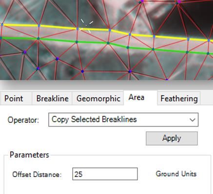
Copy Selected Breaklines
A new breakline editing capability that lets you copy an existing Breakline and place the copy at a specified
offset from the selected Breakline is introduced in Terrain Editor. The capability can be accessed from the
Terrain Editor Operators drop down menu, which is available in the Terrain Editing Panel.

Editing Breakline Vertices
Breakline vertex editing capability is enhanced. Breakline vertices can now be edited in the same way as
editing mass points. Selecting the breakline that the vertex is part of is no longer necessary.

4 October 2019                                                                                                  35
Dynamic update of Contours during Breakline editing
Contours are now dynamically updated as breaklines are being edited, giving users an immediate feedback of
the effects of the edits that is being made. Prior to ERDAS IMAGINE 2020, contours get dynamically edited
while points are being edited, but were not updated when editing a breakline until the editing until the breakline
is completed. With this update, contours are dynamically updated when either points and/or breakline are
being edited.

Consistent Style Library locations
ERDAS IMAGINE 2020 now looks for style libraries only in the associated subdirectories of the etc directory in
each of our "hives" ($PERSONAL, C:/ProgramData/ERDAS/ERDAS IMAGINE 2020, $IMAGINE_HOME). The
software no longer looks directly in $PERSONAL or etc or in the sub-directories outside of etc (e.g.
$IMAGINE_HOME/Colors or $PERSONAL/LineStyles).

    •   Arrow styles: etc/Arrows
    •   Colors: etc/Colors
    •   Fill styles: etc/FillStyles
    •   Line styles: etc/LineStyles
    •   Symbols: etc/symbols
    •   Text styles: etc/TextStyles

If you have customized style libraries stored in any of the old locations you need to move them to the new
locations in order to use them in ERDAS IMAGINE 2020 or later.

4 October 2019                                                                                                 36
System Requirements
ERDAS IMAGINE
64-bit: Intel 64 (EM64T), AMD 64, or equivalent
Computer/ Processor
(Multi-core processors are strongly recommended)
Memory (RAM) 16 GB or more strongly recommended
• 6 GB for software
Disk Space • 7 GB for example data
• Data storage requirements vary by mapping project 1
• Windows 10 Pro (64-bit) 4
Operating Systems 2, 3
• Windows Server 2016 (64-bit)
• Windows Server 2019 (64-bit)
• OpenGL 2.1 or higher (this typically comes with supported graphics cards 5)
• Java Runtime 1.7.0.80 or higher - IMAGINE Objective requires JRE and can utilize any
installed and configured JRE of version 1.7.0.80 or higher.
• Python 3.6.x or 3.7.x (Python is optionally usable with Spatial Modeler).
Software • Microsoft DirectX® 9c or higher
• .NET Framework 4.0
• OpenCL 1.2 with a device that supports double precision (cl_khr_fp64) if wanting to GPU
accelerate NNDiffuse and other Operators
• An NVIDIA card with CUDA capabilities is recommended for use with Deep Learning
Recommended Graphics
• NVIDIA® Quadro® K5200, K5000, K4200, K4000, K2200, K600, K420 6
Cards for Stereo Display
Recommended Stereo • 120 Hz (or above) LCD Monitors with NVIDIA 3D Vision™ Kit, or 3D PluraView system from
Display Monitors Schneider Digital 7
All software installations require:
• One Windows-compatible mouse with scroll wheel or equivalent input device
• Printing requires Windows-supported hardcopy devices 8
Software security (Hexagon Geospatial Licensing 2020) requires one of the following:
• Ethernet card, or
• One USB port for hardware key
Advanced data collection requires one of the following hand controllers: 9
• TopoMouse™ or TopoMouse USB™
• Immersion 3D Mouse
Peripherals
• MOUSE-TRAK
• Stealth 3D (Immersion), S3D-E type, Serial Port
• Stealth Z, S2-Z model, USB version
• Stealth V, S3-V type (add as a serial device)
• 3Dconnexion SpaceMouse Pro 10
• 3Dconnexion SpaceExplorer mouse 10
• EK2000 Hand Wheels
• EMSEN Hand Wheels
• Z/I Mouse
4 October 2019 37You can also read