Predicting In-game Actions from Interviews of NBA Players
←
→
Page content transcription
If your browser does not render page correctly, please read the page content below
Predicting In-game Actions from Interviews
                                        of NBA Players

                                        Nadav Oved ∗
                                        nadavo@campus.technion.ac.il
                                        Amir Feder ∗
arXiv:1910.11292v3 [cs.CL] 1 Jul 2020

                                        feder@campus.technion.ac.il
                                        Roi Reichart
                                        roiri@ie.technion.ac.il

                                        Sports competitions are widely researched in computer and social science, with the goal of under-
                                        standing how players act under uncertainty. While there is an abundance of computational work
                                        on player metrics prediction based on past performance, very few attempts to incorporate out-of-
                                        game signals have been made. Specifically, it was previously unclear whether linguistic signals
                                        gathered from players’ interviews can add information which does not appear in performance
                                        metrics. To bridge that gap, we define text classification tasks of predicting deviations from mean
                                        in NBA players’ in-game actions, which are associated with strategic choices, player behavior
                                        and risk, using their choice of language prior to the game. We collected a dataset of transcripts
                                        from key NBA players’ pre-game interviews and their in-game performance metrics, totalling
                                        in 5,226 interview-metric pairs. We design neural models for players’ action prediction based
                                        on increasingly more complex aspects of the language signals in their open-ended interviews.
                                        Our models can make their predictions based on the textual signal alone, or on a combination
                                        of that signal with signals from past-performance metrics. Our text-based models outperform
                                        strong baselines trained on performance metrics only, demonstrating the importance of language
                                        usage for action prediction. Moreover, the models that employ both textual input and past-
                                        performance metrics produced the best results. Finally, as neural networks are notoriously
                                        difficult to interpret, we propose a method for gaining further insight into what our models have
                                        learned. Particularly, we present an LDA-based analysis, where we interpret model predictions
                                        in terms of correlated topics. We find that our best performing textual model is most associated
                                        with topics that are intuitively related to each prediction task and that better models yield higher
                                        correlation with more informative topics.1

                                         ∗ Authors contributed equally.
                                         1 Code is available at: https://github.com/nadavo/mood
1. Introduction
Decision theory is a well-studied field, with a variety of contributions in economics,
statistics, biology, psychology and computer science (Berger 1985; Einhorn and Hog-
arth 1981). While substantial progress has been made in analyzing the choices agents
make, prediction in decision making is not as commonly researched, partly due to its
challenging nature (Gilboa 2009). Particularly, defining and assessing the set of choices
in a real-world scenario is difficult, as the full set of options an agent faces is usually
unobserved, and her decisions are only inferred from their outcomes.
One domain where the study of human action is well defined and observable
is sports, in our case Basketball. Professional athletes are experts in decision making
under uncertainty, and their actions, along with their outcomes, are well-documented
and extensively studied. While there are many attempts to predict game outcomes in
Basketball, including win probability, players’ marginal effects and the strengths of
specific lineups (Ganguly and Frank 2018; Coate 2012), they are less focused on the
decisions of individual players.
Individual player actions are difficult to predict as they are not made in lab condi-
tions and are also a function of "soft" factors such as their subjective feelings regarding
their opponents, teammates and themselves. Moreover, such actions are often made
in response to the decisions their opponents and teammates make. Currently, sports
analysts and statisticians that try to predict such actions do so mostly through past
performances, and their models do not account for factors such as those mentioned
above (Kaya 2014).
However, there is an additional signal, ingrained in fans’ demand for understand-
ing the players current state - pre-game interviews. In widely successful sports such
as baseball, football and basketball, top players and coaches are regularly interviewed
before and after games. These interviews are usually conducted to get a glimpse of how
they are currently feeling and allow them to share their thoughts, given the specifics of
the upcoming game and the baggage they are carrying from previous games. Following
the sports psychology literature, we wish to employ these interviews to gain an insight
about the players’ emotional state and its relation to actions (Uphill, Groom, and Jones
2014).2
In the sports psychology literature, there is a long standing attempt to map the
relationship between what this literature defines as "emotional state" and performance.
The most popular account of such a relationship is the model of Individual Zones of
Optimal Functioning (IZOF) (Hanin 1997). IZOF proposes that there are individual
differences in the way athletes react to their emotional state, with each having an
optimal level of intensity for each emotion for achieving top performance. IZOF sug-
gests viewing emotions from a utilitarian perspective, looking at their helpfulness in
achieving individual and team goals, and aims to calibrate the optimal emotional state
for each player to perform at her best.
In this paper we build on that literature and aim to predict actions in Basketball,
using the added signal provided in the interviews. We explore a multi-modal learning
scheme, exploiting player interviews alongside performance metrics or without them.
We build models that use as input the text alone, the metrics, and both modalities
combined. As we wish to test for the predictive power of language, alone or in combi-
2 Building on this literature, we use this concept of "emotional state" freely here and note that while some
similarities exist, it is not directly mapped to the psychological literature.
2Oved*, Feder* and Reichart Predicting Actions from Interviews
nation with past performance metrics, we look at all 3 settings, and discuss the learned
representation of the text modality with respect to the "emotional state" that could be
captured through the model.
We treat the player’s deviation from his mean performance measure in recent games
as an indication to the actions made in the current game. By learning a mapping from
players’ answers to underlying performance changes we hope to integrate a signal
about their thoughts into the action prediction process. Our choice to focus on devia-
tions from the mean performance and not on absolute performance values, is also useful
from a machine learning perspective: It allows us to generalize across players, despite
the differences in their absolute performance. We leave a more in-depth discussion of
the formulation of our prediction task for later in the paper (Section 4).
Being interested in the added behavioral signal hidden in the text, we focus on the
task (Section 4) of predicting metrics that are associated in the literature with in-game
behavior and are endogenous to the player’s strategic choices and mental state: shot
success share on the offensive side, and fouls on the defensive side (Goldman and Rao
2011). We further add our own related metrics: the player’s mean shot location, his
assists to turnovers ratio, and his share of 2 point to 3 point shot attempts. We choose
to add those metrics as they are measurable on a play-by-play basis, and are interesting
measures of relative risk. We believe our proposed measures can isolate to some extent
the risk associated with specific types of decisions, such as when to pass, when to shoot
and where to do it.
Almost no single play result is a function of only one player’s action; Yet, our
positive results from models that exploit signals from individual players only (Section 7)
indicate that meaningful predictions can be made even without direct modeling of inter-
player interactions. As this is a first paper on the topic, we leave for future work an
exploration of how player interactions can be learned, noting that such an attempt will
surely entail a more complex model.3 Also, we believe that if the interviews provide a
strong signal regarding players’ in-game decisions, it should be observed even when
interactions are not explored. Hopefully, our work will encourage future research that
considers interactions as well.
We collected (Section 3) a dataset of 1,337 interviews with 36 major NBA players
during a total of 14 seasons. Each interview is augmented with performance measures of
the player in each period (quarter) of the corresponding game. To facilitate learnability,
we focus on NBA all-stars as they are consistently interviewed before games, and
have played key roles throughout their career. Also, the fact that many players in our
dataset are still active and are expected to remain so in the following years, gives us an
opportunity to measure our model’s performance and improve it in the future.
We start by looking at a regression model as a baseline for both the text-only and
the metrics-only schemes. Then, we experiment with structure-aware neural networks
for their feature learning capabilities and propose (Section 5) models based on LSTM
(Hochreiter and Schmidhuber 1997) and CNN (LeCun et al. 1998). Finally, to better
model the interview structure and to take advantage of recent advancements in con-
textual embeddings, we also use a BERT-based architecture (Vaswani et al. 2017; Devlin
et al. 2019) and explore the trade-off between a light-weight attention mechanism and
more parameter heavy alternatives (Section 5).
3 There are novel attempts to estimate players’ partial effect on the game (Gramacy, Taddy, and Tian 2017),
which comprises of estimating the difference they make on final game outcomes. However, in this
research we decided to focus on metrics that can be attributed to specific types of decisions and not to
overall game outcomes.
3Our results (Sections 6, 7) suggest that our text-based models are able to learn
from the interviews to predict the player’s performance metrics, while the performance-
based baselines are not able to predict much better than a coin flip or the most common
class, a phenomenon we try to explain in Section 7.
Interestingly, the models that exploit both the textual signal and the signal from
past performance metrics improve on some of the most challenging predictions. These
results are consistent with the hypothesized relationship of mental state and perfor-
mance, and support claims in the literature that such an "emotional state" has predictive
power on player performance (Lazarus 2000; Hanin 2007).
Our contributions to the sports analytics and NLP literature are as follows: (1) We
provide the first model, as far as we know, that predicts player actions from language;
(2) Our model is the first that can predict relative player performance without relying on
past performance; (3) On a more conceptual level, our results suggest that the player’s
"emotional state" is related to player performance.
We support our findings with a newly-proposed approach to qualitative analysis
(Section 8). As neural networks are notoriously difficult to directly interpret, we choose
to analyse text-based NN models via topic modeling of the texts associated with the
model’s predictions. Alternative approaches for model explanations do not allow for
reasoning over higher-level concepts such as topics. Hence, we believe this could be a
beneficial way to examine many neural models in NLP and view this as an additional
contribution we present in this paper.
This analysis includes a comparison of our best performing models and finds that
our BERT-based model is most associated with topics that are intuitively related to each
prediction task, suggesting that the hypothesized "emotional state" from the sports psy-
chology literature could have been learned. Additionally, we find that this correlation
becomes stronger as the confidence of the model in its prediction increases, meaning
that a higher probability for such topics corresponds to higher model confidence. Fi-
nally, we compare our models and observe that better performing models yield higher
correlation with more informative topics.
In conclusion, we believe that this paper provides evidence for the transmission
of language into human actions. We demonstrate that our models are able to predict
real world variables via text, extending a rich NLP tradition and literature about tasks
such as sentiment analysis, stance classification and intent detection that also extract
information regarding the text author. We hope this research problem and the high level
topic will be of interest to the NLP community. To facilitate further research we also
release our data and code.
2. Related Work
Previous work on the intersection of language, behavior and sports is limited due to the
rarity of relevant textual data (Xu, Yu, and Hoi 2015). However, there is an abundance of
research on predicting human decision making (e.g. (Rosenfeld and Kraus 2018; Plonsky
et al. 2017; Hartford, Wright, and Leyton-Brown 2016)), on using language to predict
human behavior (Sim, Routledge, and Smith 2016; Niculae et al. 2015) and on predicting
outcomes in Basketball (Ganguly and Frank 2018; Cervone et al. 2014). Since we aim to
bridge the gap between the different disciplines, we survey the relevant work in each.
4Oved*, Feder* and Reichart Predicting Actions from Interviews
2.1 Prediction and Decision Making
Previous decision making work is both theoretical – modelling the incentives individ-
uals face and the equilibrium observed given their competing interests (Gilboa 2009),
and empirical – aiming to disentangle causal relationships that can shed light on what
could be driving actions observed in the world (Angrist and Pischke 2008; Kahneman
and Tversky 1979).
While there are some interesting attempts at learning to better predict human
action (Hartford, Wright, and Leyton-Brown 2016; Wright and Leyton-Brown 2010; Erev
and Roth 1998), the task at hand is usually addressed in lab conditions or using synthetic
data. In a noisy environment it becomes much harder to define the choice set, that is the
alternatives the agent faces, and to observe a clear outcome, the result of the action
taken. In our setting we can only observe proxies to the choices made, and they can
only be measured discretely, whenever a play is complete. Moreover, we can not easily
disentangle the outcome of the play from the choices that drove it, since actions are
dependent on both teammates and adversaries.
Our work attempts to integrate linguistics signals into a decision prediction pro-
cess. Language usage seems to be informative about the speaker’s current state of
mind (Wardhaugh 2011) and his personality (Fasold and Stephens 1990). Yet, this is
rarely explored in the context of decision making (Gilboa 2009). Here we examine
whether textual traces can facilitate predictions in decision making.
2.2 NLP and Prediction of Human Behavior
NLP algorithms, and particularly Deep Neural Networks (DNNs), often learn a low
dimensional language representation with respect to a certain objective and in a manner
which preserves valuable information regarding the text or the agent producing it. For
example, in sentiment analysis (Pang, Lee, and Vaithyanathan 2002) text written by
different authors is analyzed with respect to the same objective of determining whether
the text conveys positive or negative sentiment. This not only reveals something about
the text, but also about the author – her personal stance regarding the subject she
was writing about. One can view our task to share some similarity with sentiment
classification as both tasks aim to learn something about the emotional state of the
author of a given text.
Yet, a key difference between the two tasks, which poses a greater challenge in our
case, is that in our task the signal we are aiming to capture is not clearly visible in the
text, and requires inferring more subtle or abstract concepts than positive or negative
sentiment. Given a movie review, an observer can guess if it is positive or negative
rather easily. In our case, it is unclear where in the text is the clue regarding the players’
mental state, and it is even less clear how it will correspond to their actions. Moreover,
the text in our task involves a form of structured dialog between two speakers (the
player and the interviewer), which entails an additional level of complexity, on top of
the internal structures present for each speaker independently.
In a sense, our question is actually broader. We want to examine whether textual
traces can help us in the challenging problem of predicting human action. There is
a long standing claim in the social sciences that one could learn information about a
person’s character and his behavior from their choice of language (Fasold and Stephens
1990; Wardhaugh 2011; Bickerton 1995), but this claim was not put to test in a real
world setting such as those we are testing in. Granted, understanding character from
language and predicting actions from language are quite different. However, if it is the
5case that neural networks could learn a character-like context using the final action as
the supervision sign, it could have substantial implications for language processing and
even the social sciences.
In the emerging field of computational social science, there is a substantial effort
to harness linguistic signals to better answer scientific questions (Danescu-Niculescu-
Mizil et al. 2013). This approach, a.k.a text-as-data, has led to many advancements in the
prediction of stock prices (Kogan et al. 2009), understanding of political discourse (Field
et al. 2018) and analysis of court decisions (Goldwasser and Daumé III 2014; Sim,
Routledge, and Smith 2016). Our work adds another facet to this literature, trying to
identify textual signals that enable the prediction of actions which are not explicitly
mentioned in the text.
2.3 Prediction and Analysis in Basketball
Basketball is at the forefront of sports analytics. In recent decades, there have been im-
mense efforts to document every aspect of the game in real-time, and currently for every
game there is data capturing each play’s result, player and ball movements and even
crowd generated noise. Researchers have employed this data to solve prediction tasks
about game outcomes (Ganguly and Frank 2018; Kvam and Sokol 2006), points and per-
formance (Cervone et al. 2014; Sampaio et al. 2015), and possession outcome (Cervone
et al. 2016).
Recent work has also explored mechanisms that facilitate the analysis of the deci-
sions players and coaches make in a given match (Kaya 2014; Bar-Eli and Tractinsky
2000). Some have tried to analyze the efficiency and optimality of decisions across the
game (Goldman and Rao 2011; Wang et al. 2018), while others have focused on the
decisions made in the final minutes of the game, when they are most critical (McFarlane
2018). Also, attempts were made to model strategic in-game interactions in order to sim-
ulate and analyze counterfactual scenarios (Sandholtz and Bornn 2018) and to under-
stand the interplay in dynamic space creation between offense and defense (Lamas et al.
2015). We complement this literature by making text-based decision-related predictions.
We address the player’s behavior and current mental state as a factor in analyzing his
actions, while previous work in sports analytics focused only on optimality considera-
tions. Following the terminology of the sports psychology literature, we attempt to link
players emotional/mental state, as manifested in the interviews, to the performance,
actions and risk taking in the game (Hanin 1997; Uphill, Groom, and Jones 2014).
3. Data
We created our dataset with the requirement that we have enough data on both actions
and language, from as many NBA seasons as possible and for a variety of players. While
the number of seasons is constrained by the availability of transcribed interviews, we
had some flexibility in choosing the players. To be able to measure a variety of actions
and the corresponding interviews across time, we chose to focus on players that were
important enough to be interviewed repeatedly and crucial enough for their team so
that they play throughout most of the game. These choices allowed us to measure player
performance not only at the game level, but also in shorter increments, such as the
period level.
Our dataset is therefore a combination of two resources: (1) A publicly available
play-by-play dataset, collected from basketball-reference.com; and (2) The pub-
licly available interviews at ASAPsports.com, collected only for players that were
6Oved*, Feder* and Reichart Predicting Actions from Interviews
interviewed in more than three different seasons. Interviews were gathered from the
2004 − 2005 basketball season up until June 2018. As this dataset comes from a fairly
unexplored domain with regards to NLP, we follow here with a basic description of
the different sources. For a more detailed description and advanced statistics such
as common topics, interview length and player performance distributions, please see
Tables 2, 3 and 4.
We processed the play-by-play data to extract individual metrics for each player
in each game for which that player was interviewed. The metrics were collected at
both the game and the period level (see Section 4 for the description of the metrics).
We aggregated the performance metrics at the period level, to capture performance at
different parts of the game and reduce the effects of outliers.4 This is important since
performance in the first quarter could have a different meaning than performance in
the last, where every mistake could be irreversible. Each interview consists of question-
answer pairs for one specific player, and hence properties like the interview length
and the length of the different answers are player specific. Key players are interviewed
before each game, but we have data mostly for playoff games, since they were the ones
that were transcribed and uploaded.5 This bias makes sense since playoff interviews
are more in-depth and they attract a larger audience. Overall, our dataset consists of
2, 144 interviews, with some players interviewed twice between consecutive games.
After concatenating such interviews we are left with 1, 337 interviews from 36 different
players, and the corresponding game metrics for each interview. The total number of
interview-period metric pairs is 5, 226.
We next describe our in-game play-by-play data and the pre-game interviews, along
with the processing steps we apply to each.
3.1 In-game Play-by-Play
Basketball data is gathered after each play is done. As described in our "basketball
dictionary" in Table 1, a play is any of the following events: Shot, Assist, Block, Miss,
Free Throw, Rebound, Foul, Turnover, Violation, Time-out, Substitution, Jump Ball and
Start and End of Period. We ignore Time-outs, Jump Balls, Substitutions and Start/End
of Period plays as they do not add any information with respect to the metrics that
we are monitoring. If a shot was successful, there could be an assist attributed to the
passing player. Also, we observe for every foul the affected player and the opponent
charged, as well as the player responsible for each shot, miss, free-throw and lost ball.
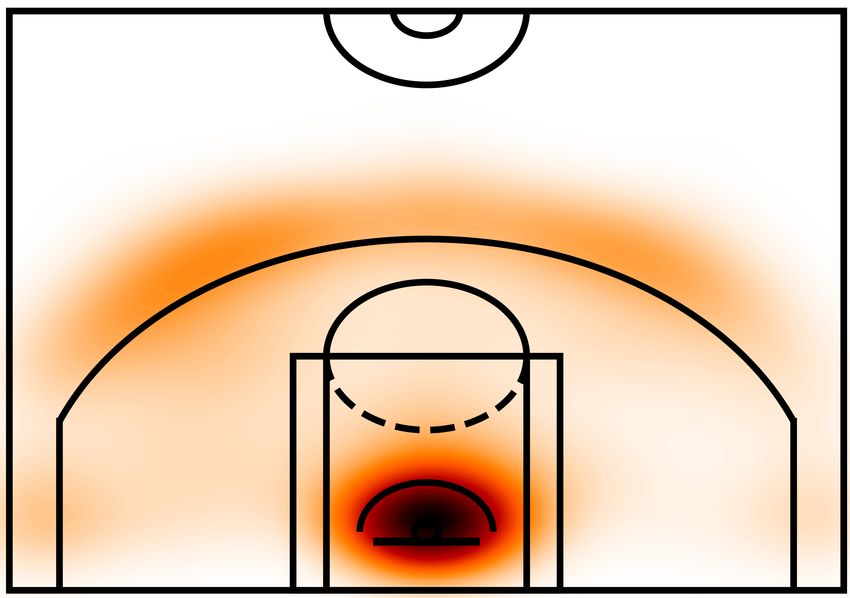
For every shot taken, there are two location variables, indicating the shot’s coordinates
on the court, with which we calculate relative distance from the basket (see Figure 1).
We use those indicators to produce performance metrics for each period.
For each event there are 10 variables indicating the 5 player lineup per team, which
we use to monitor whether a player is on court at any given play. In a typical NBA
game, there are about 450 plays. Since we are only collecting data for key players, they
are present on court during the vast majority of the game, totalling in an average of
337 plays per player per game, for an average of 83 plays per period. For each period,
we aggregate a player’s performance through the following features: Points, Assists,
Turnovers, Rebounds, Field goals made and missed, Free throws made and missed and
4 There are 4 periods in a Basketball game, not including overtime. We do not deal with overtime
performance as it might be less affected by the player pre-game state, and more by the happenings in the
4 game periods.
5 See Subsection 3.2 for an explanation on NBA playoffs.
7Term Description
Shot Attempting to score points by throwing the ball through the
basket. Each successful shot is worth 3 points if behind the 3
point arc, and 2 otherwise.
Assist Passing the ball to a teammate that eventually scores without first
passing the ball to any other player.
Block Altering an attempted shot by touching the ball while still in the
air.
Free Throw Unopposed attempts to score by shooting from behind the free
throw line. Each successful free throw is worth one point.
Rebound Obtaining the ball after a missed shot attempt.
Foul Attempting to unfairly disadvantage an opponent through cer-
tain types of physical contact.
Turnover A loss of possession by a player holding the ball.
(Shot Clock) Failing to shoot the ball before the shot clock expires. Results in
Violation a turnover to the opponent team.
Time-out A limited number of clock stoppages requested by a coach or
mandated by the referee for a short meeting with the players.
Substitution Replacing one player with another during a match. In basketball,
substitutions are permitted only during stoppages of play, but
are otherwise unlimited.
Jump Ball A method used to begin or resume the game, where two oppos-
ing players attempt to gain control of the ball after an official
tosses it into the air between them.
Period NBA games are played in four periods (quarters) of 12 minutes.
Overtime periods are five minutes in length. The time allowed
is actual playing time; the clock is stopped while the play is not
active.
Table 1: Descriptions for Basketball terms used in our dataset. Explanations and
rules derived from the official NBA rule-book at: https://official.nba.com/
rulebook/, and the Basketball Wikipedia page at: https://en.wikipedia.org/
wiki/Basketball
mean and variance of shot distance from basket, for both successful and unsuccessful
attempts. We build on these features to produce metrics that we believe capture the
choice of actions made by the player (see Section 4). Table 2 provides each player’s mean
and standard deviation values for all performance metrics. The table also provides the
average and standard deviation of the metrics across the entire dataset, information that
we use to explain some of our findings in Section 7 and modeling decisions in Section 4.
3.2 Pre-game Interviews
NBA players are interviewed by the press before and after games, as part of their
contract with their team and with the league. The interviews take place on practice
day, which is the day before the game, and on-court before, during and after the game.
An NBA season has 82 games per team, for all 30 teams, spread across 6 months, from
October to April. Then, the top 8 teams from each conference, Eastern and Western,
8Oved*, Feder* and Reichart Predicting Actions from Interviews
Figure 1: Shot location of all attempted shots for all the players in our dataset. A
darker color represents more shots attempted at that location. Black lines represent the
structure of one of the two symmetric halves of an NBA basketball court.
advance to the playoffs, where teams face opponents in a knockout tournament com-
prised of a best-of-seven series. Playoff games gather much more interest, resulting in
more interviews, which are more in-depth and with much more on the line for players
and fans alike. Our dataset is hence comprised almost solely from playoff games data.
Interviews are open ended dialogues between an interviewer and a key player from
one of the teams, with the length of the answers depending solely on the players, and
the number of questions depending on both sides.6 Questions tend to follow on player
responses, in an attempt to gather as much information about the player’s state of mind
as possible. For example:
Q: "On Friday you spoke a lot about this new found appreciation you have this
postseason for what you’ve been able to accomplish. For most people getting to that
new mindset is the result of specific events or just thoughts. I’m wondering what
prompted you specifically this off-season to get to this new mindset?"
6 The most famous short response, by football player Marshawn Lynch, can be seen in:
https://www.youtube.com/watch?v=G1kvwXsZtU8
9LEBRON JAMES: "It’s not a new mindset. I think people are taking it a little further than
where it should be. Something just – it was a feeling I was after we won in Game 6 in
Toronto, and that’s how I was feeling at that moment. I’m back to my usual self."
The degrees of freedom given, result in a significant variance in interview lengths.
Sentences vary from as little as a single word to 147, and interviews vary from 4
sentences to 753. Table 3 provides aggregated statistics about the interviews in our
dataset, as well as the number of interviews, average number of Question-Answer (Q-
A) pairs, average number of sentences and average number of words for each player.
In order to give further insight, we trained an LDA topic model (Blei, Ng, and
Jordan 2003) for each player over all interviews he participated in, and present the
top words of the most prominent topic per player in Table 4. Unsurprisingly, we can
see that most topics involve words describing the world of basketball (f.e. game, play,
team, championship, win, ball, shot) and the names of other players and teams, yet
with careful observation we can spot some words relating to the player’s or team’s per-
formance in a game (f.e. dynamic, sharp, regret, speed, tough, mental, attack, defense,
zone). Generally, most topics contain similar words across players, yet some players
show interesting deviations from the "standard" topic.7
7 The LDA model is employed here for data exploration purposes only, specifically to show the general
topic distribution per player in our dataset.
10Oved*, Feder* and Reichart Predicting Actions from Interviews
Player PF PTS FGR PR SR MSD2 MSD3 # Plays
Al Horford 2.07 12.5 0.52 0.26 0.22 5.97 6.81 299.14
(1.07) (6.71) (0.18) (0.19) (0.17) (4.74) (6.69) (57.97)
Andre Iguodala 2.19 10.42 0.6 0.26 0.42 9.56 8.42 315.0
(1.44) (6.44) (0.2) (0.27) (0.22) (8.5) (6.6) (68.38)
Carmelo Anthony 3.72 22.78 0.41 0.41 0.22 5.67 6.37 354.0
(1.27) (7.38) (0.1) (0.26) (0.13) (3.61) (4.12) (51.21)
Chauncey Billups 2.84 18.42 0.5 0.23 0.41 13.7 9.54 368.61
(1.42) (5.64) (0.15) (0.21) (0.15) (13.94) (6.84) (53.57)
Chris Bosh 2.77 15.87 0.52 0.57 0.12 5.45 4.24 312.11
(1.56) (7.18) (0.19) (0.34) (0.15) (3.94) (7.25) (49.5)
Chris Paul 3.43 19.8 0.51 0.22 0.31 9.81 9.72 341.14
(1.17) (7.43) (0.1) (0.15) (0.14) (5.27) (6.45) (57.69)
Damian Lillard 2.08 27.42 0.48 0.43 0.39 10.51 9.19 370.9
(1.24) (8.07) (0.1) (0.25) (0.13) (5.73) (5.23) (39.93)
DeMar DeRozan 2.73 26.0 0.53 0.48 0.08 5.71 2.12 345.45
(1.19) (10.52) (0.09) (0.21) (0.09) (1.58) (3.64) (30.37)
Derek Fisher 3.13 8.67 0.54 0.26 0.36 13.06 7.46 282.97
(1.61) (5.04) (0.22) (0.21) (0.22) (14.27) (8.26) (60.32)
Dirk Nowitzki 2.55 24.36 0.49 0.48 0.17 7.02 8.19 359.12
(1.52) (8.29) (0.14) (0.22) (0.12) (3.01) (8.4) (61.25)
Draymond Green 4.0 13.02 0.54 0.3 0.39 8.49 7.34 359.68
(1.38) (6.59) (0.19) (0.18) (0.16) (9.61) (6.75) (47.89)
Dwyane Wade 2.88 23.07 0.5 0.4 0.09 4.49 4.25 350.26
(1.46) (8.09) (0.12) (0.18) (0.09) (2.36) (6.7) (55.72)
James Harden 2.9 23.8 0.47 0.32 0.43 9.5 8.13 351.27
(1.58) (9.69) (0.14) (0.19) (0.14) (6.08) (6.01) (66.4)
Kawhi Leonard 2.56 13.0 0.47 0.46 0.33 8.51 8.03 277.17
(1.69) (5.3) (0.18) (0.32) (0.15) (6.82) (6.08) (70.58)
Kevin Durant 2.58 28.34 0.54 0.44 0.29 8.92 9.75 378.85
(1.44) (6.86) (0.11) (0.24) (0.09) (4.13) (5.69) (52.26)
Kevin Garnett 3.0 14.83 0.54 0.44 0.02 4.7 0.0 318.31
(1.31) (5.56) (0.2) (0.33) (0.04) (2.16) (0.0) (64.31)
Kevin Love 2.33 15.75 0.44 0.47 0.44 11.0 8.13 281.58
(1.34) (9.17) (0.15) (0.27) (0.16) (7.95) (4.79) (58.15)
Klay Thompson 2.51 19.34 0.48 0.45 0.48 16.17 8.92 352.96
(1.49) (8.65) (0.11) (0.28) (0.15) (14.97) (4.18) (58.37)
Kobe Bryant 2.93 28.07 0.48 0.38 0.24 8.21 7.6 373.7
(1.59) (7.1) (0.09) (0.2) (0.13) (4.21) (5.91) (53.15)
Kyle Lowry 3.33 21.56 0.49 0.3 0.48 14.09 8.94 334.67
(1.32) (9.9) (0.14) (0.2) (0.17) (11.57) (3.97) (46.15)
Kyrie Irving 2.44 25.2 0.52 0.37 0.28 9.19 11.49 339.68
(1.5) (8.34) (0.11) (0.19) (0.14) (5.8) (7.31) (70.44)
Lamar Odom 3.92 12.29 0.52 0.4 0.14 3.06 3.94 309.29
(1.64) (5.19) (0.18) (0.27) (0.14) (2.49) (7.82) (56.57)
LeBron James 2.49 28.75 0.53 0.34 0.22 5.81 8.2 380.43
(1.39) (8.66) (0.12) (0.16) (0.1) (3.27) (6.07) (56.21)
Manu Ginobili 3.02 14.84 0.5 0.39 0.44 9.6 7.98 276.0
(1.24) (7.47) (0.19) (0.24) (0.14) (7.8) (5.76) (65.68)
Pau Gasol 2.97 16.54 0.56 0.36 0.01 2.72 0.0 356.95
(1.2) (5.99) (0.14) (0.25) (0.03) (1.88) (0.0) (70.03)
Paul George 2.58 21.21 0.5 0.39 0.43 11.03 10.88 326.11
(1.54) (8.2) (0.11) (0.18) (0.11) (4.44) (5.76) (64.57)
Paul Pierce 3.62 19.56 0.52 0.47 0.31 8.2 9.12 351.69
(1.5) (7.85) (0.2) (0.24) (0.19) (5.38) (7.56) (77.83)
Rajon Rondo 2.74 12.19 0.5 0.23 0.08 3.22 3.97 354.26
(1.51) (6.53) (0.21) (0.11) (0.09) (2.27) (8.03) (59.83)
Ray Allen 2.56 14.9 0.5 0.45 0.5 13.56 9.26 342.85
(1.35) (7.28) (0.2) (0.3) (0.17) (8.91) (6.16) (71.59)
Richard Hamilton 3.61 20.83 0.5 0.36 0.07 5.1 2.32 382.09
(1.31) (6.91) (0.16) (0.25) (0.06) (2.57) (4.65) (61.51)
Russell Westbrook 2.85 24.3 0.45 0.33 0.21 5.16 6.46 363.52
(1.51) (8.54) (0.11) (0.14) (0.1) (3.28) (5.86) (55.8)
Shaquille O’Neal 3.68 15.79 0.61 0.71 0.0 1.43 0.0 275.37
(1.7) (6.96) (0.22) (0.23) (0.0) (1.08) (0.0) (89.38)
Stephen Curry 2.48 26.42 0.48 0.37 0.55 18.0 10.67 362.49
(1.36) (8.42) (0.11) (0.18) (0.11) (8.59) (4.05) (62.61)
Steve Nash 1.73 19.09 0.55 0.25 0.24 8.42 8.93 334.45
(1.2) (6.38) (0.13) (0.15) (0.12) (3.77) (7.0) (46.15)
Tim Duncan 2.65 18.43 0.51 0.46 0.01 2.55 0.44 324.07
(1.31) (7.53) (0.15) (0.28) (0.03) (1.41) (3.27) (58.05)
Tony Parker 1.65 18.02 0.52 0.32 0.1 5.27 6.45 317.44
(1.14) (6.99) (0.16) (0.19) (0.09) (3.24) (9.09) (52.21)
dataset Average 2.791 20.214 0.511 0.38 0.265 7.347 6.922 336.77
dataset Std. 1.489 9.438 0.153 0.239 0.204 6.054 6.771 66.44
Table 2: Performance metric mean and standard deviation (in parentheses) per player
in our dataset. We report here the actual values of the performance metrics rather than
deviations from the mean. For the definition of the performance metrics, see Section 4.
11Player # of Avg. Avg. Avg.
Interviews # of # of # of
Q-A pairs sentences words
Al Horford 14 6.43 45.29 685.4
Andre Iguodala 26 12.69 111.08 1888.6
Carmelo Anthony 18 14.28 86.78 1075.8
Chauncey Billups 31 12.19 92.81 1545.6
Chris Bosh 47 11.53 97.96 1311.2
Chris Paul 35 12.49 82.66 1165.4
Damian Lillard 12 7.92 69.0 1115.5
DeMar DeRozan 11 14.36 84.91 1259.1
Derek Fisher 39 6.87 54.0 1149.7
Dirk Nowitzki 33 12.15 114.39 1737.7
Draymond Green 59 14.97 140.88 2161.9
Dwyane Wade 72 18.93 173.58 2494.7
James Harden 30 10.73 63.77 858.6
Kawhi Leonard 18 8.5 37.5 462.9
Kevin Durant 67 17.73 138.25 2094.2
Kevin Garnett 29 11.72 92.45 1459.1
Kevin Love 24 11.79 89.54 1508.6
Klay Thompson 53 13.42 112.25 1674.9
Kobe Bryant 44 25.93 142.27 1861.1
Kyle Lowry 9 14.44 92.67 1321.8
Kyrie Irving 25 16.04 125.0 2377.6
Lamar Odom 24 10.62 61.0 805.2
LeBron James 122 22.6 189.43 2875.5
Manu Ginobili 55 8.84 68.13 1032.8
Pau Gasol 39 11.38 80.41 1281.6
Paul George 19 12.58 88.63 1220.8
Paul Pierce 32 15.28 122.78 1965.2
Rajon Rondo 27 12.04 74.19 1021.8
Ray Allen 39 8.31 63.36 1068.1
Richard Hamilton 23 12.0 63.83 1099.2
Russell Westbrook 40 18.48 108.05 1567.5
Shaquille O’Neal 19 12.63 70.53 1043.8
Stephen Curry 71 17.7 156.92 2762.9
Steve Nash 22 13.5 80.05 1132
Tim Duncan 54 13.13 86.26 1380.9
Tony Parker 55 12.75 80.84 1156.3
Dataset average 37.14 14.52 110.28 16.38
Dataset standard deviation 22.11 3.53 6.26 568.08
Table 3: Number of interviews and averages of number of Q-A pairs, sentences and
words in an interview per player in our dataset.
12Al Horford live angel trip basically beautiful allow attack next week league
Andre Iguodala year know lot rakuten see good warrior come play thing
Carmelo Anthony game tough year come kobe play court take hand back
Chauncey Billups nba teammate award twyman thank year story maurice chauncey applause
Chris Bosh really game know good team come play thing want look
Chris Paul know bowl good team really play lot shot time bowling
Damian Lillard straight breather buckle bad begin ne steph stage sick show
DeMar DeRozan smith suggest tennis talking rival skin sit sick shut shown
Derek Fisher game know play good team really feed come thing back
Dirk Nowitzki good great team time back game lot first come always
Draymond Green game thing team year know good come time really great
Oved*, Feder* and Reichart
Dwyane Wade game team play know good year come time last feel
James Harden game good know shot play open team time first point
Kawhi Leonard gear matter may minute morning normal noticing opposite order padding
Kevin Durant play know good game team come thing shot talk want
Kevin Garnett know game play thing lot team really day come want
Kevin Love game team year play lot know good last ball feel
Klay Thompson regret scary sharp sharpness shore shrug smith speed sulk thigh
Kobe Bryant game good play night come take really something much talk
Kyle Lowry challenge curious deep dynamic complete contender anything cavalier cake bucket
Kyrie Irving game play come great time moment tonight team big would
Lamar Odom really win year know last happen team good championship would
LeBron James know game year team last able time play take thing
Manu Ginobili game know tough good play sometimes see thing last happen
Pau Gasol zone really know play much game expect tonight obviously sure
Paul George know team something feel work want take together well see
Paul Pierce team know come play year game talk look really lot
Rajon Rondo game great ball team come play rebound win tonight take
Ray Allen standing mental marquis orlando operate row problem thread accustom action
Richard Hamilton relationship resolve demand record portland phone philly pay nut new
Russell Westbrook team play good great thing able game come time different
Shaquille O’Neal arena city fun would mistake lot talk back people really
Stephen Curry game play good know team kind year really time obviously
Steve Nash game really know play team back year well feel win
Tim Duncan game play good team time come back lot want really
Tony Parker good game play never rebound chance last big defense keep
Table 4: Top 10 words in the most prominent topic for each player. A topic model was trained for each player on all his interviews in the
13
Predicting Actions from Interviews
dataset.4. The Task
Our goal in this section is to define metrics that reflect the player’s in-game decisions
and actions and formulate prediction tasks based on our definitions. Naturally, the per-
formance of every player in any specific game is strongly affected by global properties
such as his skills, and is strongly correlated with his performance in recent games. We
hence define binary classification tasks, predicting whether the player is going to per-
form above or below his mean performance in the defined metrics. Across the dataset,
we found that the difference between mean and median performance is insignificant
and both statistics are highly correlated, hence we consider them as equivalent and
focus on deviation from the mean.
Different players have significantly different variances in their performance (see
Table 2) across different metrics. This phenomenon is somewhat inherent to basketball
players due to the natural variance in player skills, style and position. Due to these
evident variances, we did not attempt to predict the extent of the deviation from the
mean, but preferred a binary prediction of the direction of the deviation. Another reason
for our focus on binary prediction tasks, is that given our rather limited dataset size,
and imbalance in number of interviews per player (some players were interviewed less
than others, see Table 3), we would like our models to be able to learn across players.
That is, the training data for each player should contain information collected on all
other players, pushing us toward a prediction task that could be calculated for players
with a varying number of training examples and substantially different performance
distributions.
Performance Metrics. We consider 7 performance metrics:
1. FieldGoalsRatio(FGR)
2. MeanShotDistance2Points(MSD2)
3. MeanShotDistance3Points(MSD3)
4. PassRisk(PR)
5. ShotRisk(SR)
6. PersonalFouls(PF)
7. Points(PTS)
We denote with M = {F GR, M SD2, M SD3, P R, SR, P F, P T S} the set of performance
metrics. The performance metrics are calculated from the play-by-play data. In the
notation below p stands for a player, t for a period identifier in a specific game and
# is the count operator.8 #{event}p,t denotes the number of events of type event for
player p in a game period t. We consider the following events:
• shot: A successful shot.
• miss: An unsuccessful shot.
• 2pt: A two points shot.
• 3pt: A three points shot.
• assist: A pass to a player that had a successful shot after receiving the ball and
before passing it to any other player.
8 In the game dataset, t denotes a specific game.
14Oved*, Feder* and Reichart Predicting Actions from Interviews
• turnover: an event in which the ball moved to the opponent team due to an action
of the player.
• pf : a personal foul.
We further use the notations Distp,t for a set which contains the distances for all
the shots player p took in period t, in which the distance of that shot from the basket is
recorded, and ptsp,t for the total number of points in a certain period. Our performance
metrics, mpt , are defined for a player p in a game period t, in the following way:
M SDtp = M ean(Distp,t ) (1)
P Ftp = #{pf }p,t (2)
P T Stp = ptsp,t (3)
p,t
#{shot}
F GRtp = (4)
#{shot}p,t + #{miss}p,t
#{3pt}p,t
SRtp = (5)
(#{miss}p,t + #{shot}p,t )
#{turnover}p,t
P Rtp = (6)
#{assist}p,t + #{turnover}p,t
For MSD we consider two variants, MSD2 and MSD3, for the mean distance of 2 and 3
points shots, respectively.
4.1 Prediction Tasks
For each metric m we define the player’s mean as:
PT p p
p t=1 mt
m̄ = (7)
|T p |
where T p is the set of periods in which the player p participated. We further define the
per-metric label set Y m as:
1, mpt ≥ m̄p
Y m= {ytp,m |p ∈ P, t ∈ T }, ytp,m= (8)
0, otherwise
where P is the set of players and T is the set of periods.9
For each player p and period t, we denote with xpt the player’s interview text prior to
the game of t, and with ytp,m the label for performance metric m. In addition, lagged per-
p,m
formance metrics are denoted with yt−j , ∀j ∈ {1, 2, ..., k} (k = 3 in our experiments).10
We transform each sample in our dataset into interview-metric tuples, such that for a
given player p and period t we predict ytp,m given either:
9 Since mpt is hardly ever equal to m̄p , the meaning of ytp,m = 0 is almost always a negative deviation from
the mean.
10 lagged performance metrics refer to the same metric for the same player in the previous periods.
15(a) xpt : for the text-only mode of our models.
p,m
(b) {yt−j |∀j ∈ {1, 2, ..., k}, ∀m ∈ M }: for the metric only mode.
(c) {xpt , yt−j
p,m
|∀j ∈ {1, 2, ..., k}, ∀m ∈ M }: for the joint text and metric mode.
While in this paper we consider an independent prediction task for each perfor-
mance metric, these metrics are likely to be strongly dependent (Vaz de Melo et al. 2012).
Also, we look at each player’s actions independently, although there are connections
between actions of different players and between different actions of the same player.
We briefly discuss observed connections between our models for different tasks and
their relation to the similarity between tasks in Section 7. However, as this is the first
paper for our task, we do not attempt to model possible interactions between different
players or between metrics which often occur in team sports, and leave these to be
explored in future work.
4.2 Performance Measures and Decision Making
Our paper is about the transmission of language into actions. In practice we try to
predict performance metrics that are associated with such actions. Our measures aim
to capture different aspects of the in-game actions made by players. FGR is a measure
risk for the shots attempted. SR is also a measure of risk for attempted shots, yet it
tries to capture a player’s choice to take riskier shots that are worth more points. MSD2
and MSD3 are measures of the shot location, trying to capture for a given shot type (2/3
points) how far a player is willing to go in order to score. PR considers another offensive
aspect, passes, and since it accounts for both turnovers and assists it captures part of the
risk a player is willing to take in his choice of passing. PTS is a more obvious choice,
it is the most commonly used metric to observe a player’s offensive performance. PF is
related to defensive decisions and is correlated with aggressive behavior.
By carefully observing the data presented in Table 2 we can see that different metrics
exhibit different levels of volatility across all players in our dataset. More volatile
metrics, such as field goals ratio (FGR), shot distance (MSD2/3) and shot risk (SR) are
rather static at the player level but differ substantially between players. This volatility
in shot related measures across players could be explained by the natural differences in
shot selection between players in different positions. For example, back-court players
generally tend to take more 3 point shots than front-court players. Events such as 3
point shots are therefore much sparser in nature for many players, and in many periods
they occur at most once if at all. This causes the MSD3 (i.e. Mean Shot Distance for
3 point shots) to be 0 many more times compared to other metrics in our dataset. This
volatility ultimately makes it harder to distinguish what drives variance in these metrics
as opposed to more consistent metrics such as PF (Personal Fouls), PTS (Points) and PR
(Pass Risk).
A possible explanation for PF and PTS being more consistent in our dataset is
that they are considered rather critical performance measures to the overall teams’
performance. Our dataset mainly consists of NBA All Stars (which are key players in
their teams), interviewed before relatively important playoff games, and thus they are
expected by their teams and fans to be more consistent in these critical measures. While
players differ substantially in terms of numbers of assists and turnovers, the pass risk
(PR) metric accounts for this by looking at the ratio, resulting in a consistent measure
across our dataset.
16Oved*, Feder* and Reichart Predicting Actions from Interviews
5. Models
Our core learning task is to predict players in-game actions from their pre-game inter-
view texts. Interviews are texts which contain a specific form of structured open-ended
turn-based dialog between two speakers - the interviewer and the interviewee, which
to a certain extent hold opposite goals in the conversation. Generally speaking, an inter-
viewer’s goal is to reveal pieces of exclusive information by giving the player a chance
to reflect on his thoughts, actions and messages. However, the player’s goal is to utilize
the opportunity of public speaking to portray his competitive agenda and strengthen his
brand, while maintaining a comfortable level of privacy. In-game performance metrics
reflect different aspects of a player’s in-game actions, which expose some information
about the variance in a player’s actions and performance between different games.
We formulated multiple binary classification tasks in Section 4, and these tasks pose
several challenges from natural language processing perspectives:
• Time Series: Almost all samples in our data come from events (playoff series) which
exhibit a certain form of time-dependence, meaning that subsequent events in
the series may impact each other. This aspect requires careful treatment when
designing our models and their features.
• Remote Supervision Signal: Our labels stem from variables (performance metrics)
which are related to the speaker of the text and are only indirectly implied in the
text. In this sense, our supervision signal refers to our input signal in an indirect
and remote manner. This is in contrast to learning to predict the deviation from
the mean based on past performance metrics, where the input and the output
are tightly connected. This is also different from tasks such as sentiment analysis
where the sentiment of the review is directly encoded in its text.
• Textual Structure: Our input consists of interviews, which exhibit a unique textual
structure of a dialog between two speakers, with somewhat opposing roles - an
interviewer and an interviewee. We are interested in capturing information from
these interviews, relevant to labels related only to the interviewee. Yet, it is not
trivial to say whether this information appears in the interviewee’s answers alone
or what type of context and information do the interviewer’s questions provide.
In light of these challenges, we design our models with 4 main questions in mind:
1. Could classification models utilize pre-game interview text to predict some of the
variance in players’ in-game performance at both game and period levels?
2. Could text be combined with past performance metrics to produce better predic-
tions?
3. How could we explicitly model the unique textual structure of interviews in order
to facilitate accurate performance prediction?
4. Could Deep Neural Networks (DNNs) jointly learn a textual representation of
their input interview together with a task classifier to help us capture textual
signals relevant to future game performance?
To tackle these questions, we chose to design metric-based, text-based and com-
bined models, and assign the −M , −T and −T M suffixes to denote them respectively.
Within each set of models, we chose to explore different modeling strategies in an
17increasing order of complexity and specialization to our task. We next provide a high
level discussion of our models, and then proceed with more specific details.
Metric-based models. We implement two standard autoregressive models, which are com-
monly used tools in time-series analysis, alongside a BiLSTM (Hochreiter and Schmid-
huber 1997) model. Both models make a prediction for the next time step (game/period)
given performance metrics from the three previous time steps. These models exhibit the
predictive power of performance metrics alone, and serve as baselines for comparison
to text-based models.
Text-based models. We design our text-based models to account for different levels of
textual structure. We start by implementing a standard Bag-of-Words text classifier
which represents an interview as counts of unigrams. We continue by implementing
a word-level CNN (LeCun, Bengio et al. 1995) model, which represents interviews
as a sequence of words in their order of appearance. We then implement a sentence-
level BiLSTM model, which represents interviews as a sequence of sentences, where
each sentence is represented by the average of its word embeddings. Finally, we chose
to implement a BERT (Devlin et al. 2019) model, which accounts for the interview
structure by representing interviews as sequences of question-answer pairs. Each pair’s
embeddings are learned jointly by utilizing the model’s representations for pairs of
sequences, which are based on an attention mechanism (Vaswani et al. 2017) defined
over the word-level contextual embeddings of the question and the answer. This serves
as an attempt to account for the subtler context a question induces over an answer, and
for the role of each speaker in the dialog. These text-based models exhibit the predictive
power of text alone in our prediction task.
Combined models. DNNs tranform their input signals into vectors and their computations
are hence based on matrix calculations. This shared representation of various input sig-
nals makes theses models highly suitable to multi-task and cross-modal learning, as has
been shown in a variety of recent NLP works (e.g. (Søgaard and Goldberg 2016; Rotman,
Vulić, and Reichart 2018; Malca and Reichart 2018)). We therefore implemented variants
of our best performing LSTM and BERT text-based models which incorporate textual
features from the pre-game interview with performance metrics from the previous three
time steps. These models help us quantify the marginal effect of adding textual features
in predicting the direction of the deviation from the player’s mean performance, over
metric-based models. We next describe each of our models in details.
5.1 Metric-based Autoregressive Models
An autoregressive (AR(k)) model is a representation of a type of a random process. It is
a commonly used tool to describe time-varying processes, such as player performance.
The AR model assumes that the output variable (ytp,m ) depends linearly on its own k
previous values and on a stochastic term t (the prediction error) (Akaike 1969). We
focus on AR(3) to prevent loss of data for players with very few examples (previous
games) in our dataset:
3
X
ytp,m = c + p,m
ϕj yt−j + t (9)
j=1
18Oved*, Feder* and Reichart Predicting Actions from Interviews
We also consider using all lagged metrics as features for predicting a current metric:
3 X
X
ytp,m = c + ϕw p,w
j yt−j + t (10)
j=1 w∈M
That is, we make predictions for a given game t, player p and metric m, based on
performance in the previous k = 3 games, using either the same metric m (Equation 9)
or all metrics in M (Equation 10).
We employed a standard linear regression and a logistic regression. We tested both
models for all k values for which we had enough data, and k = 3 was chosen since it
performed best in development data experiments. We report results only for the linear
regression model, since both models performed similarly.
5.2 The BoW and TFIDF Text Classifiers
The bag-of-words (BoW) and term frequency-inverse document frequency
(TFIDF) (Salton 1991) models are standard for text classification tasks (Yogatama
and Smith 2014), and they therefore serve as our most basic text-based models.
We constructed both BoW and TFIDF feature vectors per interview, and have tried
using unigrams and bigrams, alone or in combination. We considered Random Forest
(RF) (Liaw, Wiener et al. 2002), Support Vector Machine (SVM) (Cortes and Vapnik 1995)
and Logistic Regression (LR) (Ng and Jordan 2002) classifiers. While BoW provides
a straight-forward effective way to represent text, it assumes n-gram (in our case we
tried n = 1, n = 2, n = 1, 2) independence and therefore does not take the structure of
the text into account. TFIDF adjusts for the fact that some words are more frequent in
general, but makes the same assumptions. We report results for the Random Forest (RF)
classifier for both BoW (unigrams) and TFIDF (unigrams + bigrams) feature sets, since
these consistently performed better in development data experiments, for BoW and
TFIDF respectively. Finally, since these simple models were consistently outperformed
by our best text-based DNN models (see Section 7), we did not attempt to incorporate
any performance metrics as features into them.
5.3 Deep Neural Networks
DNNs have proven effective for many text classification tasks (Kim 2014; Ziser and
Reichart 2018). An appealing property of these models is that training a DNN using a
supervision signal results not only in a predictive model, but also with a representation
of the data in the context of the supervision signal. This is especially intriguing in our
case, where the supervision signal is not clearly visible in the text, and is more related
to its speaker.
Moreover, the text in our task is structured as a dialog between two speakers, which
entails an additional level of contextual dependence between speakers, on top of the
internal linguistic structures of the utterances produced by the individual speakers.
These factors pose a difficult challenge from a modeling perspective, yet DNNs are
known for their architectural flexibility which allows learning a joint representation for
more than one sequence (Chen, Bolton, and Manning 2016), and have shown promising
performance in different tasks where models attempt to capture nuanced phenomena
in text (Peters et al. 2018).
19We consider three models that excel on text classification tasks: CNN (Kim 2014),
BiLSTM (Hochreiter and Schmidhuber 1997) and BERT (Devlin et al. 2019). In order
to obtain a vectorized representation of an interview’s text, we employed different
text embedding techniques per model, each based on different pre-trained embedding
models. Below we describe the various models.
5.3.1 The CNN Model
Motivation. We implement a standard word-level CNN model for text classification
(CNN-T), closely following the implementation described in (Kim 2014). This model
showed promising results on various text classification tasks such as sentiment classifi-
cation and stance detection (Kim 2014). By implementing this model we aim to examine
the extent to which a standard word-level text classification neural network, which does
not explicitly account for any special textual structure except for the order of the words
in the text, can capture our performance metrics from text.
Model Description. Interviews are fed into the model as a sequence of words in their
order of appearance in the interview. We concatenated the interview’s word embed-
ding vectors into an input matrix, such that embeddings of consequent words appear
in consequent matrix columns. Since interviews vary in length, we padded all word
matrices to the size of the longest interview in our dataset. We then employed three 2D
convolution layers with max-pooling and a final linear classification layer.
5.3.2 The BiLSTM Models
Motivation. Our CNN model treats an interview as a single sequence of words, and apart
from the fact that the order of words is maintained in the input matrix, it does not model
any textual structure. By implementing BiLSTM-based models we aim to directly model
the interview as a sequence of sentences, rather than of words. We believe that since
interviews involve multiple speakers interacting in the form of questions and answers,
where each question and answer are comprised of multiple sentences, a sequential
sentence-level model could capture signals word-level models cannot.
We chose to implement our text-based BiLSTM (LSTM-T) as a sentence-level se-
quential model, where each sentence is represented by the average of its pre-trained
word embeddings (Adi et al. 2016). Since BiLSTM is a general sequential model, it also
fits naturally as an alternative time-series model for performance metrics only (LSTM-
M), similar to the AR(k) model described in Equation 10. The various model variants
allow us to examine the independent effects of text and metrics on our prediction
tasks, using the same underlying model. Moreover, we can now examine the effect
of combining text and metric features together in a BiLSTM model (LSTM-TM) by
concatenating the metric feature vectors used as input to LSTM-M with the final textual
vector representation produced by LSTM-T (see Figure 2).
Model Description. We next provide the technical implementation details of each of our
BiLSTM-based models.
LSTM-T. The BiLSTM model for text is fed with the sentences of the interview, in their
sequential order. Each sentence is represented by the average of its word embeddings.
The BiLSTM’s last hidden-state forward and backward vectors are concatenated and
fed into two linear layers with dropout and batch normalization, and a final linear
classification layer (see the left part of Figure 2).
20You can also read